MODAL ANALYSIS - the Dept. of Mechanical Engineering at - Vrije ...

MODAL ANALYSIS
Patrick Guillaume, Department of Mechanical Engineering,Vrije Universiteit Brussel, Pleinlaan
2, B-1050 Brussel, Belgium.
Keywords: Vibration, Estimation, Frequency domain, Modal analysis, Modal parameters, Natural
frequency, Damping, Mode shapes, Transfer function, SISO, MIMO, Mechanical systems, SDOF,
MDOF.
Contents
1. Introduction
2. The “Modal” Model
2.1. Single Degree of Freedom
2.2. Multiple Degree of Freedom
2.2.1. Mode Shapes and Operating Deflection Shapes
2.2.2. Observability and Controllability of Modes
3. Frequency-Domain Identification of Modes
3.1. Least-Squares Estimation
3.1.1. Common-Denominator Model
3.1.2. Linearity in the Parameters
3.1.3. Normal Equations
3.1.4. Reduced Normal Equations
3.1.5. Stabilization Chart
3.2. Maximum Likelihood Estimation
3.2.1. Gauss-Newton Optimization
3.2.2. Confidence Intervals
4. Application
5. Conclusion
Glossary
DOF: Degree of freedom.
FRF: Frequency response function.
GTLS: Generalized total least squares.
IQML: Iterative quadratic maximum likelihood.
IRF: Impulse response function.
LS: Least squares.
LSCE: Least squares complex exponential.
MDOF: Multiple-degree-of-freedom.
ML: Maximum likelihood.
MIMO: Multiple-input-multiple-output
SDOF: Single-degree-of-freedom.
SISO: Single-input-single-output.
TLS: Total least squares.

Summary
In this contribution the applicability of frequency-domain estimators in the field of modal analysis
will be illustrated. The basics of vibration and modal analysis are briefly summarized. In modal
analysis, mechanical systems with a few inputs and hundreds of outputs have to be identified. This
requires adapted frequency-domain estimators designed to handle large amount of data in a
reasonable amount of time. A practical example will be given and finally the conclusions will be
drawn.
1. Introduction
It is well known that (mechanical) structures can resonate, i.e. that small forces can result in
important deformation, and possibly, damage can be induced in the structure.
Figure 1: Tacoma Narrows Bridge Disaster.
The Tacoma Narrows bridge disaster (Figure 1) is a typical example of this. On November 7, 1940,
the Tacoma Narrows suspension bridge collapsed due to wind-induced vibration (i.e. flutter).
Situated on the Tacoma Narrows in Puget Sound, near the city of Tacoma, Washington, the bridge
had only been open for traffic a few months.
Wings of airplanes can be subjected to similar flutter phenomena during flight. Before an airplane is
released, flight flutter tests have to be performed to detect possible onset of flutter. The classical
flight flutter testing approach is to expand the flight envelope of a airplane by performing a
vibration test at constant flight conditions, curve-fit the data to estimate the resonance frequencies
and damping ratios, and then to plot these frequencies and damping estimates against flight speed or
Mach number. The damping values are then extrapolated in order to determine whether it is save to
proceed to the next flight test point. Flutter will occur when one of the damping values tends to
become negative. Before starting the flight tests, ground vibration tests as well as numerical
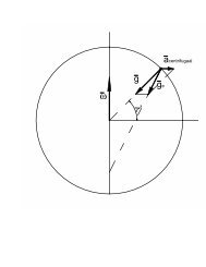
simulations and wind tunnel tests (see Figure 2) are used to get some prior insight into the problem.

(a) (b)
Figure 2: Wind tunnel tests on a scaled model of (a) a Cessna and (b) an Airbus A380.
The majority of structures can be made to resonate, i.e. to vibrate with excessive oscillatory motion.
Resonant vibration is mainly caused by an interaction between the inertial and elastic properties of
the materials within a structure. Resonance is often the cause of, or at least a contributing factor to
many of the vibration and noise related problems that occur in structures and operating machinery.
To better understand any structural vibration problem, the resonant frequencies of a structure need
to be identified and quantified. Today, modal analysis has become a widespread means of finding
the modes of vibration of a machine or structure (Figure 3). In every development of a new or
improved mechanical product, structural dynamics testing on product prototypes is used to assess its
real dynamic behavior.
2. The “Modal” Model
Figure 3: Modal analysis of a car body.
Modes are inherent properties of a structure, and are determined by the material properties (mass,
damping, and stiffness), and boundary conditions of the structure. Each mode is defined by a natural
(modal or resonant) frequency, modal damping, and a mode shape (i.e. the so-called “modal
parameters”). If either the material properties or the boundary conditions of a structure change, its
modes will change. For instance, if mass is added to a structure, it will vibrate differently. To
understand this, we will make use of the concept of single and multiple-degree-of-freedom systems.

2.1 Single Degree of Freedom
A single-degree-of-freedom (SDOF) system (see Figure 4 where the mass m can only move along
the vertical x-axis) is described by the following equation
m � x�
( t)
+ cx�
( t)
+ kx(
t)
= f ( t)
(1)
with m the mass, c the damping coefficient, and k the stiffness. This equation states that the sum of
all forces acting on the mass m should be equal to zero with f (t)
an externally applied force,
− m�x �(t)
the inertial force, − c� x(t)
the (viscous) damping force, and − kx(t)
the restoring force. The
variable x (t)
stands for the position of the mass m with respect to its equilibrium point, i.e. the
position of the mass when f ( t)
≡ 0 . Transforming (1) to the Laplace domain (assuming zero initial
conditions) yields
Z ( s)
X ( s)
= F(
s)
(2)
with Z (s)
the dynamic stiffness
2
Z ( s)
= ms + cs + k
(3)
The transfer function H (s)
between displacement and force, X ( s)
= H ( s)
F(
s)
, equals the inverse
of the dynamic stiffness
1
H ( s)
= (4)
2
ms + cs + k
Figure 4: SDOF system.
2
The roots of the denominator of the transfer function, i.e. d ( s)
= ms + cs + k , are the poles of the
system. In mechanical structures, the damping coefficient c is usually very small resulting in a
complex conjugate pole pair
λ = −σ
± iω
(5)
d
with f = ω 2π
the damped natural frequency,
d
d
f = ω 2π
the (undamped) natural frequency where ω = k m = λ , and
n
n
ζ = c 2 mωn
= σ λ the damping ratio ( f d = f n
2
1 − ζ ).
If, for instance, a mass Δ m is added to the original mass m of the structure, its natural frequency
decreases to ω n = k ( m + Δm)
. If c = 0 , the system is not damped and the poles becomes purely
imaginary, λ = ± iωn
.
n

The Frequency Response Function (FRF), denoted by H (ω)
, is obtain by replacing the Laplace
variable s in (4) by i ω resulting in
1
1
H ( ω)
= =
(6)
2
2
− mω
+ icω
+ k ( k − mω
) + icω
Clearly, if c = 0 , then H (ω)
goes to infinity for ω → ω k m (see Figure 4).
Although very few practical structures could realistically be modeled by a single-degree-of-freedom
(SDOF) system, the properties of such a system are important because those of a more complex
multiple-degree-of-freedom (MDOF) system can always be represented as the linear superposition
of a number of SDOF characteristics (when the system is linear time-invariant).
2.2 Multiple Degree of Freedom
Multiple-degree-of-freedom (MDOF) systems are described by the following equation
M x�
�(
t) + Cx�
( t)
+ Kx(
t)
= f(
t)
(7)
In Figure 5, the different matrices are defined for a 2-DOF system with both DOF along the vertical
x-axis.
f 1 (t)
k 1
f 2 (t)
k 2
m 2
m 1
c 2
c 1
x 2 (t)
x 1 (t)
⎡m
M =
⎢
⎣
1
0
n =
⎡k1
+ k
K = ⎢
⎣ − k2
⎡c1
+ c
C = ⎢
⎣ − c2
0 ⎤
m
⎥
2⎦
2
2
− k
k
2
− c
Figure 5: 2-DOF system.
c
2
⎤
⎥
⎦
2
⎤
⎥
⎦
2
⎧ f1(
t)
⎫
f(
t)
= ⎨ ⎬
⎩ f2(
t)
⎭
⎧ x1(
t)
⎫
x(
t)
= ⎨ ⎬
⎩x2
( t)
⎭
Transforming (7) to the Laplace domain (assuming zero initial conditions) yields
Z( s) X(
s)
= F(
s)
(8)
with Z (s)
the dynamic stiffness matrix
2
Z ( s)
= Ms
+ Cs
+ K
(9)
The transfer function matrix H (s)
between displacement and force vectors, X ( s) = H(
s)
F(
s)
,
equals the inverse of the dynamic stiffness matrix
2
−1
N(
s)
H ( s)
= [ Ms
+ Cs
+ K]
=
d(
s)
with the numerator polynomial matrix N (s)
given by
2
N ( s ) = adj(
Ms
+ Cs
+ K)
(11)
and the common-denominator polynomial d (s)
, also known as the characteristic polynomial,
2
d ( s)
= det( M s + Cs
+ K)
(12)
(10)

When the damping is small, the roots of the characteristic polynomial d (s)
are complex conjugate
∗
pole pairs, λ m and λ m , m = 1, �,
N m , with N m the number of modes of the system. The transfer
function can be rewritten in a pole-residue form, i.e. the so-called “modal” model (assuming all
poles have multiplicity one)
= m N
R R
H ( s)
(13)
∗
m
m
∑ + ∗
m= 1 s − λm
s − λm
The residue matrices R m , m = 1, �,
N m , are defined by
R m lim H(
s)(
s − λm
)
(14)
=
s→λ
m
It can be shown that the matrix m R is of rank one meaning that R m can be decomposed as
⎧ ψ m ( 1)
⎫
⎪
ψ ( 2)
⎪
T ⎪ m ⎪
R m = m m = ⎨ ⎬⎣ψ
m ( 1)
ψ m ( 2)
� ψ m ( N m ) ⎦
(15)
⎪ � ⎪
⎪⎩
ψ m ( N m ) ⎪⎭
with m a vector representing the “mode shape” of mode m. From equation (13), one concludes
that the transfer function matrix of a linear time-invariant MDOF system with N m DOFs is the sum
of N m SDOF transfer functions (“modal superposition”) and that the full transfer function matrix is
completely characterized by the modal parameters, i.e. the poles λ m = −σ
m ± i ωd
, m and the mode
shape vectors m , m N m , , = 1 � .
Taking the inverse Laplace transform of (13) gives the Impulse Response Function (IRF)
N
∑
m=
1
∗
m
∗
m
λmt
λ t
h ( t)
R e + R e
(16)
= m
m
which consists of a sum of complex exponential functions.
2.2.1 Mode Shapes and Operating Deflection Shapes
At or near the natural frequency of a mode, the overall vibration shape (“operating deflection
shape”) of a structure will tend to be dominated by the mode shape of the resonance. Applying a
harmonic force at one of the DOFs, say r, with angular frequency corresponding to the damped
natural frequency of for instance the n-th mode, i.e. s = iω
d , n , results in a displacement vector that
is approximately equal to
nψ
n ( r)
X( ω d , n ) ≈ Fr
( ωd
, n )
(17)
σ
n
The observed displacement at angular frequency ω d , n is called an “operating deflection shapes” and
is approximately proportional to the mode shape vector of mode n, i.e. n . When σ n is small, the
proportionality is well satisfied. In reality, there will always be a (small) contribution of the other
modes resulting in
⎛
Nm
Nm
∗ ∗ ⎞
⎜ nψ
n ( r)
mψ
m ( r)
mψ
m ( r)
⎟
X ( ω d , n ) = ⎜ + ∑
+ ∑
Fr
( ωd
, n )
σ n m 1 σ m i(
ωn
ωm
) m 1 σ m i(
ωn
ω m )
⎟
(18)
⎜
= + −
= + + ⎟
⎝
m≠n
⎠

2.2.2 Observability and Controllability of Modes
Assuming, for example, that one force is applied in DOF 1 while the displacement is observed in
DOF 2. In that case, the multiple-input-multiple-output (MIMO) transfer function matrix simplifies
to the following single-input-single-output (SISO) transfer function
H
2,
1
( s)
= m N
ψ
( 2)
⋅ψ
( 1)
ψ
( 2)
⋅ψ
( 1)
∗ ∗
m m
m m
∑ +
∗
m= 1 s − λm
s − λm
If ψ n ( 1)
≠ 0 then mode n will only be “observed” in DOF 2 if ψ n ( 2)
≠ 0 . If ψ n ( 1)
= 0 then it is
clear that the terms corresponding to mode n will not appear in the sum, i.e. mode n cannot be
excited (or “controlled”) by applying a force in DOF 1. The DOFs where a mode shape vector
equals zero are called nodal points or nodes. In practice, this means that the force actuator should
not be positioned in a nodal point of the modes of interest. To reduce the risk of missing modes, the
number of excitation points can be increased. The same is true for the response measurements. The
number of inputs (excitation points) is typically in the order of 1 to 10, while the number of outputs
(response measurements) can reach more than 1000 points when using optical measurement
equipment such as for instance a scanning laser Doppler vibrometer.
3. Frequency-Domain Identification of Modes
Typical for modal analysis is the very large number of outputs. This huge amount of data requires
dedicated algorithms that balance between accuracy and memory/computing needs. In Section 3.1
such a ‘dedicated’ frequency-domain least-squares estimator will be presented. Based on these
results, it is possible to implement more sophisticated identification methods (see 6.43.8.2
Estimation with Known Noise Model and 6.43.8.4 Estimation with Unknown Noise Model) such as
for instance the frequency-domain Maximum Likelihood (ML) estimator (Section 3.2).
3.1 Least Squares Estimation
3.1.1 Common-Denominator Model
The relationship between output o ( o = 1, �,
N o ) and input i ( i = 1, �,
N i ) is modeled in the
frequency domain by means of a common-denominator transfer function
ˆ N k ( ω)
H k ( ω)
= (20)
d(
ω)
for k = 1, �,
N o N i (where k = ( o −1)
N i + i ) and with
k
n
∑
j=
0
N ( ω ) = Ω ( ω)
B
(21)
j
kj
the numerator polynomial between output o and input i and
n
∑
j=
0
d(
ω ) = Ω ( ω)
A
(22)
j
j
the common-denominator polynomial. The real-valued coefficients j A and B kj are the parameters
to be estimated. Several choices are possible for the polynomial basis functions Ω j (ω)
. For a
discrete-time domain model, the functions Ω j (ω)
are usually given by Ω j ( ω ) = exp( −iωTs
⋅ j)
j
(with T s the sampling period) while for a continuous-time domain model Ω ( ω ) = ( iω)
. The bad
j
(19)

numerical conditioning of the continuous-time domain approach can be improved by using for
instance orthogonal Forsythe polynomials (at the expense of an increase of the computation time).
3.1.2 Linearity in the Parameters
In modal analysis, measurements of Frequency Response Functions (FRFs) are commonly used (see
6.43.8.1 Measurements of Frequency response functions). Replacing the model H ˆ ( ω)
in (20) by
the measured FRFs H k ( ω f ) for f N f , , = 1 � gives, after multiplication with the denominator
polynomial,
n
∑ ∑
Ω ( ω ) B − Ω ( ω ) H ( ω ) A ≈ 0
(23)
j f kj
j=
0 j=
0
n
j
f
k
f
j
with o i N N k , , 1 � = and f N f , , = 1 � . Because the equations (23) are “linear-in-the-parameters”,
they can be reformulated as
with
⎡X
⎢
0
⎢
⎢ �
⎢
⎣
0
1
k
0
X
0
2
�
�
X
⎧Bk
0 ⎫
⎪ ⎪
⎪Bk
1 ⎪
= ⎨ ⎬ ,
⎪ � ⎪
⎪⎩
B ⎪ kn ⎭
0
0
N N
o
i
Y
Y
Y
�
1
2
N N
o
⎧A0
⎫
⎪ ⎪
⎪ A1
⎪
= ⎨ ⎬
⎪ � ⎪
⎪⎩
A ⎪ n ⎭
i
⎧
⎤ ⎪
⎥ ⎪
⎥ ⋅ ⎨
⎥
⎪
⎥
⎦
⎪
⎪⎩
�
1
2
N N
o
i
⎫
⎪
⎪
⎬ ≈ 0
⎪
⎪
⎪⎭
⎡ W
⎤
k ( ω1
)[ Ω0
( ω1
) , Ω1
( ω1
) , �,
Ωn
( ω1
) ]
⎢
⎥
X k = ⎢
�
⎥
(26)
⎢
⎥
⎣
Wk
( ω N )[ Ω0
( ω ) , Ω1
( ) , , Ω ( ) ]
f
N ω
f
N � f
n ω N f ⎦
⎡ −W
⎤
k ( ω1)[
Ω0(
ω1)
H k ( ω1
) , Ω1
( ω1
) H k ( ω1
) , �,
Ωn
( ω1
) H k ( ω1
) ]
⎢
⎥
Y k = ⎢
�
⎥ (27)
⎢
⎥
⎣
−Wk
( ω N )[ Ω0
( ω ) ( ) , Ω1
( ) ( ) , , Ω ( ) ( ) ]
f
N H
f k ω N ω
f
N H
f k ω N � f
n ω N H
f k ω N f ⎦
Note that every equation in (23) has been weighted with a frequency-dependent function Wk ( ω f ) .
The quality of the estimates can often be improved by using an adequate weighting function. The
(complex) Jacobian matrix J of this least-squares problem
⎡X1
⎢
0
J = ⎢
⎢ �
⎢
⎣
0
0
X
0
2
�
�
X
0
0
N N
o
i
Y
Y
Y
�
1
2
N N
o
⎤
⎥
⎥
⎥
⎥
⎦
i
has Nf No Ni rows and (n+1)(No Ni +1) columns (with Nf >> n, where n is the order of the
n = 2N
).
polynomials, m
k
(24)
(25)
(28)

3.1.3 Normal Equations
Many estimators used in modal analysis form the normal equations explicitly, i.e. they compute
Re( J J)
H
explicitly. Note that the real part of J J
H has to be taken because the coefficients are real.
Deriving the estimates directly from the Jacobian matrix leads to a better-conditioned problem.
However, forming the normal equations can result in a faster implementation, as will be the case
here too. The normal equations can be written as
⎡R1
⎢
0
⎢
⎢ �
⎢
T
⎢S1
⎣
S
0
R
2
T
2
�
�
�
S1
⎤ ⎧
⎪
S
⎥
2 ⎥ ⎪
� ⎥ ⋅ ⎨
⎥ ⎪
Tk
⎥ ⎪
⎦ ⎩⎪
NoN
i
∑
k=
1
�
1
2
N N
o
i
⎫
⎪
⎪
⎬ ≈ 0
⎪
⎪
⎪⎭
H
H
H
with R k = Re( X k X k ) , S k = Re( X k Yk
) , and T k = Re( Yk
Yk
) . The entries of these matrices equal
⎛
R ⎜
k ( r,
s)
= Re
⎜
⎝
⎛
T ⎜
k ( r,
s)
= Re
⎜
⎝
N
f
∑
f = 1
⎛
S
⎜
k ( r,
s)
= − Re
⎜
⎝
N
N
f
∑
f
∑
f = 1
W
f = 1
k
W
k
( ω )
k
f
f
f
⋅Ω
k
H
r−1
W ( ω ) H ( ω )
2
( ω )
2
k
f
( ω ) Ω
f
f
⋅Ω
s−1
H ( ω ) ⋅Ω
2
H
r−1
H
r−1
⎞
( ω ⎟ f )
⎟
⎠
( ω ) Ω
( ω ) Ω
f
f
s−1
s−1
⎞
( ω ⎟ f )
⎟
⎠
⎞
( ω ⎟ f )
⎟
⎠
If a discrete time-domain model is used, i.e. Ω j ( ω f ) = exp( −iω
f Ts ⋅ j)
, and if the frequencies are
uniformly distributed (i.e. ω f = f ⋅ Δω
, f N f , , 1 � = , with summations can be rewritten as
Δ ω = 2π
NTs
), then, the above
⎛
R ⎜
k ( r,
s)
= Re
⎜
⎝
⎛
T ⎜
k ( r,
s)
= Re
⎜
⎝
N
f
∑
f = 1
⎛
S
⎜
k ( r,
s)
= − Re
⎜
⎝
N
N
f
∑
f
∑
f = 1
W
f = 1
k
W
k
( ω )
k
f
f
f
⋅ e
k
i2π
( r−s
) f N
W ( ω ) H ( ω )
2
( ω )
2
k
f
f
⋅ e
⎞
⎟
⎠
H ( ω ) ⋅e
2
i2π
( r−s
) f N
i2π
( r−s
) f N
⎞
⎟
⎠
⎞
⎟
⎠
One can readily verify that the above matrices have a Toeplitz structure and that their entries can be
time-efficiently computed with the Fast Fourier Transform (FFT) algorithm.
3.1.4 Reduced Normal Equations
Although the number of rows of the normal matrix in (29) is much smaller than the number of rows
of the Jacobian matrix (28), its size is still quite huge (i.e. (n+1)(No Ni +1) rows and columns). As
we are mainly interested in a fast and stable method to construct a stabilization chart (see next
section), only the denominator coefficients (i.e. the poles) are in fact required. Elimination of the
numerator coefficients
yields
⎡
⎢
⎣
k
−1
= −R
⋅S
⋅
NoN
i
∑
k=
1
k
k
T −1
⎤
Tk − Sk
⋅ R k ⋅ Sk
⎥ ⋅ ≈ 0
⎦
(29)
(30)
(31)
(32)
(33)

N
T −1 or M ⋅ ≈ 0 with M = ∑ T − ⋅ ⋅
k=
1 k Sk
R k Sk
. The size of the square matrix M is n+1, and thus
o i N
much smaller than the original normal equation (29). To remove the parameter redundancy of
transfer function model (20) (and to avoid the trivial solution with all coefficient equal to zero), a
constraint has to be imposed on the coefficients of the transfer functions. This can be done, for
instance, by imposing that one of the coefficients is equal to a non-zero constant value. Assume, for
instance, that the last coefficient of � is constrained to 1 (i.e. coefficient n+1). In that case, the
Least Squares (LS) estimate of � is given by
ˆ
LS
−1
⎧ − [ M(
1:
n, 1:
n)]
⋅{
M(
1:
n,
n + 1)}
⎫
= ⎨
⎬
⎩
1
⎭
Once ˆ LS is known, (32) can be used to derive all ˆ
LS coefficients. This approach is more time
2 2
efficient that solving (29) directly (approximately o i N N times faster). The mode shape vectors are
derived using (14) and (15).
3.1.5 Stabilization chart
In modal analysis, a stabilization chart is an important tool that is often used to assist the user in
separating physical poles from mathematical ones. A stabilization chart is obtained by repeating the
analysis for increasing model order n. For each model order, the poles are calculated from the
estimated denominator coefficients. The stable poles (i.e. the poles with a negative real part) are
then presented graphically in ascending model order in a so-called “stabilization chart” (see Figure
6). Estimated poles corresponding to physically relevant system modes tend to appear for each
estimation order at nearly identical locations, while the so-called mathematical poles, i.e. poles
resulting from the mathematical solution of the normal equations but meaningless with respect to
the physical interpretation, tend to jump around. These mathematical poles are mainly due to the
presence of noise on the measurements.
(a) (b)
Figure 6. Stabilization chart obtained with (a) a time-domain estimator (LSCE) and
(b) the frequency-domain least-squares estimator.
The LSCE estimator (Least Squares Complex Exponential) is probably the most frequently used
technique in industry. The LSCE estimator is a time-domain technique that makes use of impulse
response functions (16) to derive the modal parameters. In Figure 6 the stabilization chart of the
LSCE estimator is compared with the proposed frequency-domain least squares estimator. It turns
out that in many applications, the frequency-domain estimator is able to generate quite clear
stabilization compared to the LSCE approach.
(34)

3.2 Maximum Likelihood Estimation
3.2.1 Gauss-Newton Optimization
Assuming the FRFs to be uncorrelated, the (negative) log-likelihood function reduces to
NoN
N i f Hˆ
k ( , ω f ) − H k ( ω f )
� ML(
) = ∑∑
(35)
var{ H ( ω )}
k=
1 f = 1
k f
2
T T T T
The Maximum Likelihood (ML) estimate of = [ 1 , �,
No
N , ] is obtained by minimizing (35).
i
This can be done by means of a Gauss-Newton optimization algorithm, which takes advantage of
the quadratic form of the cost function (35). The Gauss-Newton iterations are given by
(a)
(b)
solve Re( J
set
p+1
=
H
p
p
J
p
+
)
p
p
= − Re( J
with r p = r(
p ) , J = ∂r(
) ∂ and
p
p
H
p
r
p
)
for
p
⎧ Hˆ
⎫
11(
, ω1)
− H11(
ω1)
⎪
⎪
⎪ var{ H11(
ω1)}
⎪
⎪
⎪
r( ) = ⎨
� ⎬
(37)
⎪ Hˆ
N ( , ) − ( ) ⎪
oN
ω
i N H
f NoN
ω i N f
⎪
⎪
⎪ var{ H N ( )}
⎩
oN
ω i N f ⎪⎭
The Jacobian matrix J p has the same structure as the matrix J given in (28). Also here it is possible
H
H
to form the normal equations (i.e. Re( J p J p ) and Re( J p rp
) ) in a similar time-efficient way as
presented in Section 3.1. See 6.43.8.2 Estimation with Known Noise Model and 6.43.8.4 Estimation
with Unknown Noise Model for more information about frequency-domain ML identification.
3.2.2 Confidence Intervals
A good approximation of the covariance matrix of the ML estimate ˆ
ML is obtained by inverting the
Fisher information matrix (see 6.43.8. Frequency Domain System Identification)
ˆ
cov{
ML
} ≈ [ 2 Re( J J
H
∞
∞
)]
−1
with J ∞ the Jacobian matrix evaluated in the last iteration step of the Gauss-Newton optimization.
As one is mainly interested in the uncertainty on the modal frequencies and damping ratios, only the
covariance matrix of the denominator coefficients is in fact required. Starting from (38), one can
show that this matrix is given by
ˆ
cov{
ML
}
⎡
⎢2
⎣
≈ ∑ i oN N
k=
1
−1
(36)
(38)
T −1
⎤
T k − Sk
⋅ R k ⋅ Sk
⎥
(39)
⎦
with R k , S k , and T k as defined in Section 3.1.3 but now applied to Re( J ∞ J ∞ )
H
. Hence, it is not
necessary to invert the full matrix occurring in (38). From (39), it is possible to compute the
uncertainty on the modal frequencies and damping ratios. For flight flutter testing – but also for
applications such as vibration-based fault detection and operational modal analysis – the availability
of reliable estimates together with confidence intervals is important.

4. Application
In this section, modal analysis will be applied to a slat track, which is safety critical component of a
airplane. Slat tracks (see Figure 7) are located at the leading edge of an aircraft wing and make part
of a gliding mechanism that is used to enlarge the wing surface. The enlargement of the wing
surface is needed in order to increase the lift force at reduced velocity during landing and take off.
A slat track of an Airbus A320 airplane is considered here. The A320 airplane has 5 slats per wing.
The first slat (i.e. the inboard slat between fuselage and engine) contains 4 slat tracks. The other 4
slats have 2 slat tracks each. Safety critical components such as slat tracks are rigorously tested to
prove their ability to withstand all safety regulations. It is commonly accepted that the track should
outlive the plane by five times. Using computer simulations, it is possible to predict the lifetime of
a track using Finite Element (FE) models. To validate the dynamic behavior of these FE models,
experimentally obtained estimates of the modal parameters are required.
SLAT TRACK
LEADING
EDGE
OF WING
SLAT TRACK
SLAT
Figure 7: Mounted slat track on an Airbus A320 in extended position.
FORCE SENSOR
STINGER
SHAKER
SHAKER
SCANNING LASER
DOPPLER VIBROMETER
(a) (b) (c)
Figure 8: Measurement setup. (a) Excitation with a shaker. (b) Response measurements with a
scanning laser Doppler vibrometer. (c) Measurement points on the surface of the slat track.
In Figure 8(a) a shaker is used to excite the slat track with a multisine signal. A multisine is a
periodic signal consisting of a sum of sine waves at uniformly distributed frequencies (from 0 Hz to
8192 Hz in this case with a resolution of 1 Hz). A force sensor is attached on the slat track and is in
contact with the shaker through a stinger. The stinger has the characteristic of being stiff in only
one direction, i.e. that of the intended excitation. In this example, one surface of the track is

measured by means of a scanning laser Doppler vibrometer (see Figure 8(b); the shaker is at the
backside of the slat track, which is vertically suspended by means of a elastic rope). The FRF
measurements are performed in 500 points uniformly distributed over the surface of one side of the
slat track (see Figure 8(c)).
Starting from the FRF measurements, the modal parameters can be estimated using the frequencydomain
estimator given in Section 3. In the considered frequency band, a few hundreds of modes
are present. Figure 9 shows 4 of the estimated mode shapes (with enlarged displacement
amplitudes). The real displacements are of the order of a few micrometers.
(a) (b)
(c) (d)
Figure 9: Mode shapes of the slat track for a modal frequency of
(a) 4091 Hz, (b) 4161 Hz, (c) 4739 Hz, and (d) 5169 Hz

5. Conclusions
In this contribution about modal analysis, a ‘dedicated’ multivariable implementation for frequencydomain
estimators, based on a common-denominator transfer function model, has been given.
Typical for modal analysis is the very large number of outputs. This huge amount of data requires
dedicated algorithms that balance between accuracy and memory/computing requirements.
The results given in this contribution can be generalized to other frequency-domain estimators such
as the Total Least Squares (TLS), Generalized Total Least Squares (GTLS), Iterative Quadratic
Maximum Likelihood (IQML), … (see 6.43.8.2 Estimation with Known Noise Model and 6.43.8.4
Estimation with Unknown Noise Model).
Bibliography
Ewins D.J. (2000). Modal Testing: Theory, Practice and Application, Hertfordshire: Research
Studies Press. [In this book, all the steps involved in planning, executing, interpreting and applying
the results from a modal test are described in straightforward terms.]
Ewins D.J. and Inman D.J., Editors (2001). Structural Dynamics @ 2000: Current Status and
Future Directions, Baldock: Research Studies Press. [This book presents an integrated collection of
contributions on structural dynamics.]
Heylen W., Lammens S. and Sas P. (1998). Modal Analysis Theory and Testing, KULeuven (ISBN:
90-73802-61-X). [This book gives a good introduction to the theory as well as all practical aspects
of experimental modal analysis.]
Inman D.J. (1994). Engineering Vibration, Englewood Cliffs: Prentice Hall. [This book gives an
introduction to mechanical systems and vibration.]
Maia N.M.M. and Silva J.M.M., Editors (1997). Theoretical and Experimental Modal Analysis,
Taunton: Research Studies Press. [This book takes an advanced and up-to-date look at modal
analysis. The basics of vibration theory and signal processing are discussed.]
Pintelon R. and Schoukens J. (2001). System Identification: A Frequency Domain Approach, IEEE
Press and John Wiley & Sons (ISBN 0-7803-6000-1). [This book presents a general approach to
system identification, with both practical examples and theoretical discussions.]