Curved Folding - Computer Graphics Laboratory
Curved Folding - Computer Graphics Laboratory
Curved Folding - Computer Graphics Laboratory

Create successful ePaper yourself
Turn your PDF publications into a flip-book with our unique Google optimized e-Paper software.
Martin Kilian<br />
TU Vienna<br />
Evolute<br />
Simon Flöry<br />
TU Vienna<br />
Evolute<br />
<strong>Curved</strong> <strong>Folding</strong><br />
Zhonggui Chen<br />
TU Vienna<br />
Zhejiang University<br />
Niloy J. Mitra<br />
IIT Delhi<br />
Alla Sheffer<br />
UBC<br />
Helmut Pottmann<br />
TU Vienna<br />
Figure 1: Top left: Reconstruction of a car model based on a felt design by Gregory Epps. Close-ups of the hood and the rear wheelhouse are<br />
shown on the left. The fold lines are highlighted on the car’s development. Top right and bottom: Architectural design. All shown surfaces<br />
can be isometrically unfolded into the plane without cutting along edges and can thus be texture mapped without any seams or distortions.<br />
Abstract<br />
Fascinating and elegant shapes may be folded from a single planar<br />
sheet of material without stretching, tearing or cutting, if one incorporates<br />
curved folds into the design. We present an optimizationbased<br />
computational framework for design and digital reconstruction<br />
of surfaces which can be produced by curved folding. Our<br />
work not only contributes to applications in architecture and industrial<br />
design, but it also provides a new way to study the complex<br />
and largely unexplored phenomena arising in curved folding.<br />
CR Categories: I.3.5 [<strong>Computer</strong> <strong>Graphics</strong>]: Computational Geometry<br />
and Object Modeling—Geometric algorithms, languages,<br />
and systems; I.3.5 [<strong>Computer</strong> <strong>Graphics</strong>]: Computational Geometry<br />
and Object Modeling—Curve, surface, solid, and object representations<br />
Keywords: computational differential geometry, computational<br />
origami, architectural geometry, industrial design, developable surface,<br />
folding, curved fold, isometry, digital reconstruction.<br />
1 Introduction<br />
Developable surfaces appear naturally when spatial objects are<br />
formed from planar sheets of material without stretching or tearing.<br />
Paper models such as origami art are prominent examples.<br />
The striking elegance of models folded from paper, such<br />
as those by David Huffman [Wertheim 2004], arises particularly<br />
from creases known as curved folds. Such folds can be generated<br />
from a single planar sheet. Early investigations of curved<br />
folds are due to Huffman [1976]. More recently, computational<br />
geometers became interested in folding problems and computational<br />
origami [Demaine and O’Rourke 2007]. Their work concentrates<br />
on piecewise linear structures; according to [Demaine and<br />
O’Rourke 2007], ‘little is known’ in the curved case. While industrial<br />
designers have started to explore the technique of curved folding<br />
(www.curvedfolding.com), current geometric modeling systems<br />
still lack any support for such a design process (in fact, most<br />
CAD systems are lacking a proper treatment of developable surfaces).<br />
As a result, Frank O. Gehry, who favors developable shapes<br />
for many of his architectural designs (cf. [Shelden 2002]), has initiated<br />
the development of a CAD module for developable surfaces<br />
by his technology company. To the best of our knowledge, curved<br />
folding is not present in that module either.<br />
Motivated by the potential and interest in the use of curved folding<br />
for various geometric design purposes, we investigate this topic<br />
from the perspective of geometric modeling.<br />
Related work. Developable surfaces are well studied in differential<br />
geometry [do Carmo 1976]. They are surfaces which can be unfolded<br />
into the plane while preserving the length of all curves on the
Figure 2: The car model of Figure 1 and its development (top<br />
right). The patch decomposition into torsal ruled surfaces is shown<br />
using the following color scheme: planes are shown in yellow,<br />
cylinders in green, cones in red, and tangent surfaces in blue. Sample<br />
rulings are shown on some patches of the windshield and the<br />
side window. Such a segmentation is essential for NURBS surface<br />
fitting and manufacturing.<br />
surface. Developable surfaces are composed of planar patches and<br />
patches of ruled surfaces with the special property that all points<br />
of a ruling have the same tangent plane. Such torsal ruled surfaces<br />
consist of pieces of cylinders, cones, and tangent surfaces, i.e., their<br />
rulings are either parallel, pass through a common point, or are tangent<br />
to a curve (curve of regression), respectively. Whereas a torsal<br />
ruled surface has only one continuous family of rulings, general<br />
smooth developable surfaces are usually a much more complicated<br />
combination of patches. The presence of planar parts is the main<br />
source of this huge variety of possibilities. The level of difficulty is<br />
further increased if one admits creases, i.e., curved folds (see Figure<br />
2).<br />
In geometric design, various ways of treating developability have<br />
been pursued: as a constraint in tensor product B-spline surfaces<br />
of degree (n, 1) [Chu and Sequin 2002; Aumann 2004], aiming<br />
only at approximate developability [Pérez and Suárez 2007], viewing<br />
the surfaces as sets of their tangent planes [Pottmann and Wallner<br />
2001], subdividing strips of planar quads [Liu et al. 2006], or<br />
computing with triangle meshes and a local convexity constraint<br />
[Frey 2004; Wang and Tang 2004; Subag and Elber 2006; Wang<br />
2008]. Bo and Wang [2007] model paper strips as rectifying developables<br />
of one of their geodesics. Digital reconstruction of torsal<br />
ruled surfaces employing a plane-geometric approach is the topic<br />
of [Peternell 2004].<br />
Mesh parametrization and segmentation using developable surfaces<br />
has been investigated in [Julius et al. 2005] and [Yamauchi et al.<br />
2005]. Rose et al. [2007] show how to compute developable surfaces<br />
from boundary curves, and present a strategy for selecting an<br />
optimal solution. Several algorithms have been proposed for the<br />
construction of papercraft models [Mitani and Suzuki 2004; Massarwi<br />
et al. 2006; Shatz et al. 2006] using folds along line segments.<br />
In all these papers, triangle meshes are used to represent<br />
developable surfaces.<br />
Only a few contributions deal with the difficult analysis and computation<br />
of creases in developable surfaces. Most of them concentrate<br />
on conical creases [Kergosien et al. 1994; Cerda et al. 1999; Frey<br />
2004]. Starting from conical folds, Cerda et al. [2004] investigated<br />
gravity-induced draping of naturally thin flat sheets.<br />
Contributions and overview. We present an optimization-based<br />
computational framework for the design and reconstruction of general<br />
developable surfaces with a strong focus on curved folding applications.<br />
Our main contributions are as follows:<br />
We employ quad meshes with planar faces as a discrete differential<br />
geometric representation of developable surfaces, and for this<br />
representation introduce new ways of computing curvatures and<br />
bending energy. Moreover, we discuss curved folds from the discrete<br />
perspective (Section 2).<br />
In Section 3, we introduce the core of our work, a novel optimization<br />
algorithm which allows us to compute developable surfaces<br />
with curved folds that are isometric to a given planar sheet,<br />
while at the same time achieving additional objectives such as approximation<br />
of given geometric data, aesthetics, and minimization<br />
of bending energy.<br />
Section 4 presents various ways in which the basic optimization<br />
algorithm can be used for design. Even simple applications lead to<br />
new results, such as modeling developable strips of minimal bending<br />
energy.<br />
Another main contribution of our work is digital reconstruction<br />
of objects exhibiting developable surfaces with curved folds. Algorithms<br />
for preprocessing the input data in order to make the algorithm<br />
of Section 3 applicable to digital reconstruction are discussed<br />
in Section 5.<br />
Combining digital reconstruction, optimization and recently introduced<br />
algorithms for computing in shape space [Kilian et al.<br />
2007] we have a rich toolbox for geometry processing with curved<br />
folds. This is demonstrated by means of a few application scenarios<br />
in Section 6. Finally, we summarize our main results, and address<br />
directions for future research within the largely unexplored area of<br />
curved folding.<br />
2 Discrete developable surfaces<br />
Developable surfaces. As our basic representation of developable<br />
surfaces we employ quad-dominant meshes with planar<br />
faces, which is also the representation of choice for discrete differential<br />
geometry [Sauer 1970; Bobenko and Suris 2005].<br />
A strip of planar quadrilaterals (Figure 3, left) is a discrete model<br />
of a torsal ruled surface. Such a ‘PQ strip’ can be trivially unfolded<br />
into the plane without distortions. The edges where successive<br />
quads join together give us the discrete rulings. In general they<br />
form the edge lines of the regression polyline r0, r1,...; in special<br />
cases the discrete rulings are parallel, or pass through a fixed point.<br />
A refinement process which maintains planarity of quads generates,<br />
in the limit, a torsal ruled surface Σ (Figure 3, right). Its rulings are<br />
the limits of the discrete rulings, which in general are tangent to the<br />
regression curve r(t), and in special cases are parallel (cylinder), or<br />
pass through a fixed point (cone).<br />
The representation of developable surfaces as PQ strips provides<br />
various advantages over triangle meshes: (i) developability is guaranteed<br />
by planarity of faces and the development is easily obtained,<br />
(ii) subdivision applied to PQ strips provides a simple and computationally<br />
efficient multi-scale approach [Liu et al. 2006], (iii) the<br />
regression curve – which is singular on the surface and thus needs<br />
to be controlled – is present in a discrete form, and (iv) the curvature<br />
behavior can be easily estimated as shown next.
Curvatures and bending energy. The rulings on a smooth developable<br />
surface constitute one family of principal curvature lines<br />
corresponding to vanishing principal curvature. The second family<br />
is given by the orthogonal trajectories of the rulings which integrate<br />
the directions of non-vanishing principal curvatures κ2. We<br />
are interested in a discrete definition of κ2, and the related bending<br />
energy Ebend = R κ 2 2dA.<br />
The rulings on a PQ strip are given by the edge lines Ri := piqi<br />
(cf. Figure 4a). As a discrete principal curvature line we take a polyline<br />
C with vertices ci 2 Ri whose edges cici+1 are orthogonal to<br />
the inner bisectors Si of Ri and Ri+1. In other words, each edge of<br />
C intersects consecutive rulings at the same angle (this definition is<br />
also motivated by an analogous definition in the context of circular<br />
meshes [Bobenko and Suris 2005]). We want to attach a surface<br />
normal vector ni to the edge midpoint mi =(ci + ci+1)/2, and<br />
take the normal vector of the plane Pi spanned by edges Ri,Ri+1<br />
for that purpose. The unit vectors fnig form the Gaussian image<br />
of C and thus it is natural to define the principal curvature κ2 at ci<br />
via:<br />
κ2(ci) :=<br />
kni − ni− 1k<br />
= Ni/Li. (1)<br />
kci − mi− 1k + kci − mik<br />
This definition has the advantage that the denominator Li can be<br />
computed in the planar development of the strip, while only the<br />
numerator Ni := kni − ni− 1k requires the embedding in space.<br />
Note that the curvature κ2 always has a positive sign, in contrast to<br />
usual definitions. As we used it in its squared form only, this does<br />
not matter.<br />
RUsing the notation of Figure 4 the discrete bending energy Ei =<br />
2<br />
κ2dA of a region bounded by two discrete principal curvature<br />
lines C, ¯ C at distance h := k¯ci − cik and two bisectors Si− 1Si<br />
(depicted by the brown highlight in Figure 4a) is given as<br />
Ei = wikni − ni− 1k 2 . (2)<br />
The weight wi associated with the ruling Ri is given by<br />
wi = h(ln ¯ Li − ln Li)/( ¯ Li − Li), (3)<br />
where Li is the denominator of Equation (1). As ¯ Li ! Li, in the<br />
limit, we get wi = h/Li. Thus the bending energy of a general PQ<br />
C<br />
n1 n1 n1<br />
n1 n1 n1<br />
P1<br />
r4<br />
c1 c1 c1<br />
c1 c1 c1<br />
r3<br />
q0<br />
c0<br />
p0<br />
r0<br />
r1<br />
r2<br />
ΣΣ<br />
n(t)<br />
n(t)<br />
n(t)<br />
n(t)<br />
n(t)<br />
r(t)<br />
Figure 3: A PQ strip (left) is a discrete model of a developable surface<br />
Σ (right). The intersections of edges piqi of adjacent planar<br />
quads generate the regression polyline ri. In the limit of a refinement<br />
process, this regression polyline becomes the regression curve<br />
r(t). Polylines C, whose edges cici+1 intersect inner bisectors of<br />
consecutive discrete rulings at right angles, are discrete versions<br />
of principal curvature lines, and serve for the definition of discrete<br />
curvatures. The unit normals to planar quads Pi are denoted by ni.<br />
(a)<br />
CC<br />
¯C¯C<br />
¯C¯C ¯C ¯C¯C<br />
¯C¯C ¯C¯C¯C¯C ¯C¯C¯C¯C<br />
pi pi pi<br />
pi pi<br />
qi<br />
qi<br />
pi pi<br />
qi<br />
qi qi qi<br />
Ri Ri Ri<br />
Ri Ri<br />
Ri+1 Ri+1 Ri+1<br />
Ri+1<br />
Ri+1<br />
Ri+1<br />
Ri+1<br />
Ri+1 Ri+1 Ri+1<br />
ci ci ci<br />
Ri Ri<br />
ci<br />
ci ci<br />
ci+1 ci+1 ci+1<br />
ci+1<br />
ci+1<br />
ci+1<br />
ci+1<br />
ci+1 ci+1 ci+1<br />
¯ci ¯ci ¯ci<br />
¯ci− 1<br />
ci ci<br />
ci− 1<br />
¯ci ¯ci ¯ci<br />
¯ci+1 ¯ci+1 ¯ci+1<br />
¯ci+1<br />
¯ci+1<br />
¯ci+1<br />
¯ci+1<br />
¯ci+1 ¯ci+1 ¯ci+1<br />
mi<br />
¯ci ¯ci<br />
mi<br />
mi mi mi<br />
Si Si Si<br />
mi− mi− mi− mi−<br />
mi−<br />
mi− mi−<br />
mi− mi− mi− 1<br />
1<br />
1<br />
1<br />
1<br />
Si<br />
Si Si Si<br />
h<br />
Si− Si− Si− Si−<br />
Si− Si−<br />
Si−<br />
Si− Si− Si− 1<br />
1<br />
1<br />
1<br />
1<br />
(b)<br />
ri<br />
(c)<br />
Li Li Li<br />
Li Li Li<br />
¯Li ¯Li<br />
¯Li ¯Li<br />
¯Li ¯Li ¯Li ¯Li<br />
¯Li ¯Li ¯Li ¯Li<br />
¯Li ¯Li ¯Li<br />
¯Li<br />
Figure 4: (a) The rulings of a PQ strip are given by the edge<br />
lines Ri := piqi. The inner bisector of RiRi+1 is denoted by<br />
Si. Edges cici+1 of the polyline C intersect Si orthogonally. If<br />
mi is the mid-point of cici+1, and ni is the normal to the plane<br />
Pi := RiRi+1, then the principal curvature at ci is naturally defined<br />
by Equation (1). (b) To avoid infinite curvatures at cone vertices,<br />
computation takes place on a slightly shrunken strip. (c) The<br />
total bending energy of a region (brown) bounded by Si− 1Si and<br />
two principal curvature lines C ¯ C is given by Equations (2), (3).<br />
strip can be simply approximated by a sum of energies Ei of the<br />
type (2). Note that we cannot directly apply known formulae for<br />
discrete bending energies [Desbrun et al. 2005] since those assume<br />
that all edge lengths tend to zero if one passes to the limit. This is<br />
not the case for the rulings in our approach.<br />
<strong>Curved</strong> folds. In the smooth setting, the following fact about<br />
curved folds is well known (see e.g. [Huffman 1976]): At each<br />
point of a fold curve c, the osculating plane of c is a bisecting<br />
plane of the tangent planes on either side of the fold. This follows<br />
immediately from the identical geodesic curvatures of the fold<br />
curve c with respect to the two adjacent developable surfaces S1<br />
and S2. Hence, given the surface on one side of a fold curve, we<br />
can compute (part of) the other as the envelope of planes, obtained<br />
by reflecting the tangent planes about the osculating planes of c.<br />
This is discussed in some detail in [Pottmann and Wallner 2001],<br />
but one finds only that part of S2 whose rulings meet c. Thus, the<br />
approach is not sufficient for most of our tasks where, in addition,<br />
multiple folds may appear, and the locations of such fold curves<br />
only become known in the process of optimization. In contrast to<br />
x<br />
∆i<br />
D2<br />
D2<br />
D2 D2 D2<br />
αi αi αi<br />
αi αi<br />
pi− pi− pi− pi−<br />
pi− pi− pi−<br />
pi− pi− pi− pi− 1<br />
1<br />
1<br />
1<br />
pi pi pi<br />
αi αi<br />
pi<br />
pi pi pi<br />
βi βi βi<br />
βi βi<br />
pi+1 pi+1 pi+1<br />
pi+1<br />
pi+1<br />
pi+1<br />
pi+1<br />
pi+1 pi+1 pi+1 βi βi<br />
D1<br />
D1<br />
D1 D1 D1<br />
Figure 5: Two PQ strips<br />
meeting at a discrete<br />
curved fold. For a given<br />
PQ strip D1, the discrete<br />
ruling of the adjacent strip<br />
D2 in a point pi lies on a<br />
quadratic cone ∆i.<br />
the smooth setting, in the discrete<br />
case there are more degrees of<br />
freedom in choosing the surface<br />
S2 as described next.<br />
As a discrete model M of a general<br />
developable surface we use a<br />
quad-dominant mesh with planar<br />
faces, where the sum of inner angles<br />
at each vertex is equal to 2π.<br />
This means that we have a bijective<br />
mapping to a planar mesh of<br />
the same combinatorics such that<br />
corresponding faces are isometric.<br />
Suppose a curved fold appears as<br />
a common polygon P of two PQ<br />
strips D1,D2 on the model M.<br />
Given the strip D1 on one side of
P , we ask about the degrees of freedom in choosing the adjacent<br />
strip D2. Clearly, we have to choose the discrete rulings in D2 so<br />
that each vertex pi 2 P exhibits the angle sum 2π. Let e− :=<br />
(pi− 1 − pi)/kpi− 1 − pik and e+ := (pi+1 − pi)/kpi+1 − pik.<br />
Let the angle sum of D1 at pi be γi = αi + βi (see Figure 5).<br />
Then, the discrete ruling vector x on D2 must form the angle sum<br />
∢(e− , x)+∢(x, e+) =2π − γi. With c := cos γi, this reads:<br />
(c 2 − 1)x 2 +(x e− ) 2 +(x e+) 2 − 2c(x e− )(x e+) =0. (4)<br />
Hence, the rulings have to lie on a quadratic cone ∆i. Note that<br />
the ruling of D1 also lies on this cone since its straight extension<br />
satisfies our requirement, though it does not describe a surface with<br />
a curved fold but a smooth extension. To obtain D2, we may take<br />
one ruling on the cone ∆i and compute further rulings at vertices<br />
pj by keeping planarity of consecutive rulings. However, most of<br />
these solutions will not be suitable since they do not discretize a<br />
smooth surface. One has to take rulings which yield ‘small’ directional<br />
changes when passing from one cone to the next one. This<br />
necessitates an optimization approach as described next.<br />
3 The basic optimization algorithm<br />
The basic optimization algorithm simultaneously optimizes a discrete<br />
developable surface M and its planar development P . To<br />
maintain isometry between corresponding faces of M and P , we<br />
originally let M be a quad-dominant soup of planar polygons M i in<br />
space. These polygons are isometric to the corresponding faces P i<br />
in the planar mesh P , see Figures 6 and 7. During the optimization,<br />
the polygon soup M will become a mesh via a registration procedure<br />
which bears some similarity to that used in the PRIMO mesh<br />
deformation tool [Botsch et al. 2006]. However, our optimization<br />
requires more sophistication since we have to simultaneously optimize<br />
the development P while satisfying various other constraints.<br />
Optimization starts with an initial set of pairs (M i ,P i ) of isometric<br />
planar polygons (primarily quads in our setting). The faces P i form<br />
a planar mesh P , while in space the corresponding polygons M i<br />
are assumed to roughly represent a developable shape D. They are<br />
not yet precisely aligned along edges. Thus M is not a mesh but<br />
a polygon soup. Later, in Sections 4 and 5, we describe how to<br />
compute initial positions P i for different applications.<br />
The unknowns. We introduce a Cartesian coordinate system in<br />
the plane of P , with origin o and basis vectors e1, e2. Each face P i<br />
of P is congruent to the respective face M i in space. For each such<br />
face, the image of (o; e1, e2) under the isometric transformation<br />
P i<br />
7! M i is a Cartesian frame (o i , e i 1, e i 2) in the plane of the<br />
face M i . If (px,py) are the coordinates of a vertex p of P i , then<br />
the corresponding vertex m of M i is m = o i + pxe i 1 + pye i 2.<br />
During the optimization, the frames (o i , e i 1, e i 2) undergo a spatial<br />
motion, and the coordinates (px,py) can also vary since we allow<br />
the polygons P i to change.<br />
We linearize the spatial motion of any face M i using an instantaneous<br />
velocity vector field: The velocity of a point x can be represented<br />
as v(x) := ¯c i + c i x, where ¯c i , c i are vectors in 3-space.<br />
e2<br />
e2 e2<br />
e2 e2<br />
e2 e2<br />
ooooo o<br />
e1<br />
e1<br />
e1 e1<br />
e1 e1<br />
e1 e1<br />
P i<br />
P i P i<br />
P i P i<br />
P i P i<br />
P i P i<br />
P i P i<br />
P i P i<br />
P i P i<br />
P i P i<br />
p<br />
o i<br />
o i o i<br />
o i o i<br />
o i o i<br />
o i o i<br />
o i o i<br />
o i o i<br />
o i o i<br />
o i o i<br />
e i<br />
e 1<br />
i e<br />
1<br />
i<br />
e1 i e<br />
1<br />
i<br />
e1 i e<br />
1<br />
i<br />
e1 i e<br />
1<br />
i<br />
e1 i e<br />
1<br />
i<br />
e1 i e<br />
1<br />
i<br />
e1 i e 1<br />
i<br />
e1 i e1 i e<br />
1<br />
i<br />
e 2<br />
i e<br />
2<br />
i<br />
e2 i e<br />
2<br />
i<br />
e2 i e<br />
2<br />
i<br />
e2 i e<br />
2<br />
i<br />
e2 i e<br />
2<br />
i<br />
e2 i e<br />
2<br />
i<br />
e2 i e 2<br />
i<br />
e2 i e2 i<br />
2<br />
D<br />
M i<br />
m 1<br />
m 2<br />
Figure 6: Basic setup for the optimization when a reference surface<br />
D is used. Faces with the same color are congruent.<br />
Mi<br />
Mi<br />
Mi Mi Mi<br />
Pi Pi Pi<br />
Pi Pi Pi<br />
Figure 7: Top left: Initial polygon soup M. Top right: Development<br />
P . Bottom left: M after subdivision and optimization. Bottom<br />
right: M after three rounds of subdivision and optimization.<br />
Figure 8: Stability of the proposed optimization strategy. After artificial<br />
perturbation of faces (left), 10 rounds of optimization yield<br />
an almost aligned polygon soup (right). The stability of the procedure<br />
allows us to use rough estimates of ruling directions and<br />
planar development to initialize the algorithm<br />
Thus a vertex m+ of the displaced quad face is given by:<br />
m+ = m + ¯c i + c i<br />
o i + px(c i<br />
e i 1)+py(c i<br />
e i 2).<br />
The new vertex position is linear in the unknown parameters<br />
¯c i , c i 2 R 3 of the velocity field, and also linear in the unknown<br />
coordinates px,py. We optimize over both the velocity parameters<br />
and the coordinates. The products pxc i and pyc i result in nonlinear<br />
terms if we insist on simultaneously optimizing them. To<br />
avoid nonlinear optimization, we alternately optimize for displacements<br />
¯c i , c i and for vertex coordinates px,py. Since our objective<br />
function is quadratic in both types of unknowns this amounts to<br />
alternately solving two sparse systems of linear equations.<br />
Applying displacements corresponding to c, ¯c destroys the exact<br />
isometric relation between corresponding faces Pi and Mi. It is<br />
therefore necessary to further modify the vertices of M i . This can<br />
either be done by rigid registration of the face P i to the estimated<br />
vertex locations m j<br />
+ as proposed by Botsch et al. [2006], or by<br />
using a helical motion as described in [Pottmann et al. 2006] – we<br />
use the former approach.<br />
The objective function. Our objective function is designed to<br />
simultaneously ensure that M becomes a mesh, fits the input data,<br />
and satisfies the aesthetic requirements of the application.
If a vertex p in the planar mesh P is shared by k faces, then p corresponds<br />
to k different vertices m 1 , . . . , m k of the corresponding<br />
k faces in M. Since these vertices should agree in the final mesh,<br />
we use a vertex agreement term of the form:<br />
Fvert := X (m i +<br />
m j<br />
+) 2 ,<br />
where the sum extends over all ` ´ k<br />
combinations per vertex p 2 P ,<br />
2<br />
and over all vertices in P .<br />
For M to approximate an underlying data surface D, we include a<br />
fitting term Ffit which is quadratic in the vertex coordinates m. Let<br />
mc denote the closest point in D to m, and let nc denote the unit<br />
normal at mc to the underlying surface. We use a linear combination<br />
of the squared distance (m mc) 2 and the squared distance to<br />
the tangent plane [(m mc) nc] 2 as the data fitting term. When<br />
fitting curves, especially near boundaries, we use tangent lines instead<br />
of tangent planes.<br />
Finally, we need a fairness term Ffair. For each pair of adjacent<br />
quads M i and M j of the PQ strip, we use the discrete bending energy<br />
of the corresponding developable surface wij(n i + n j<br />
+ )2 , as<br />
given by Equations (2) and (3), as the fairness term. The normal of<br />
a quad M i of M is given by n i = e i 1 e i 2. Under small displacements,<br />
this normal linearly varies as n i + = n i + c i<br />
n i . Given<br />
a polyline (p1, . . . pn) representing a fold line, i.e., a crease or a<br />
segment of a boundary curve, the contribution to Ffair is a sum of<br />
squared second differences P (pi 1 2pi+pi+1) 2 . Fairness terms<br />
are also applied to the respective polylines in the planar domain P .<br />
The fairness term Ffair alone is not always sufficient to maintain<br />
convex quads, and to prevent flips in the planar mesh P , especially<br />
when the quads become thin after several steps of subdivision.<br />
Hence we add another term Fconv to enforce convexity. We<br />
assume that the orientation of each face of P coincides with the<br />
orientation of the plane induced by the frame (o; e1, e2). A corner<br />
(pi 1, pi, pi+1) of a planar polygon is convex if and only if the<br />
oriented area of the triangle ∆(pi 1, pi, pi+1) is positive. This<br />
term also prevents flipping of faces.<br />
The algorithm. Combining all individual terms, our basic optimization<br />
problem reads,<br />
minimize F = Fvert + λFfit + µFfair<br />
subject to Fconv 0.<br />
We alternately minimize the objective function over new positions<br />
of vertices in P , and displacements of faces in space, i.e., velocity<br />
vectors for the corresponding face planes. Observe that the weights<br />
wij of Ffair, which only depend on the planar mesh P , remain fixed<br />
when optimizing for displacements of faces in space and the side<br />
condition Fconv is also not needed. Hence, the spatial sub-problem<br />
E1<br />
E1<br />
E1 E1 E1<br />
E2<br />
E2<br />
E2 E2 E2<br />
Figure 9: Basic setup for bending energy minimization. We start<br />
with a regular grid (left). After prescribing point locations and<br />
tangent planes at the boundary the basic optimization is applied.<br />
(Right) The result after one round of optimization.<br />
(5)<br />
Figure 10: Results of bending energy minimization for different<br />
boundary conditions. Given user constraints, the final models are<br />
obtained by alternately optimizing and subdividing.<br />
amounts to solving a sparse linear system, and subsequent application<br />
of the corresponding rigid body motion per face. Optimizing<br />
the development P is more involved since the weights wij change<br />
in a non linear way as the geometry of P changes. Additionally<br />
we have a quadratic term Fconv to maintain convexity as a side constraint.<br />
With the meshes scaled to fit inside a unit cube, we found<br />
λ = 1 and µ = 10 4 to be good values to start the optimization.<br />
Given an initial mesh P and a polygon soup M that roughly approximates<br />
a developable shape, we alternately optimize for P and<br />
M. The optimization terminates when the vertex agreement term<br />
falls below a given threshold. For the next refinement level, we subdivide<br />
the current mesh P , and map the new faces to space using<br />
the rigid transformation associated with the faces of P at the current<br />
level. The refinement process splits each quad of P to form<br />
two new ones. Splitting is performed along the edges that do not<br />
correspond to ruling directions (see Figure 3, right). The process is<br />
repeated until desired accuracy is reached.<br />
4 Applications to surface design<br />
In this section we employ the basic optimization algorithm to the<br />
design of objects with curved folds.<br />
Developable surfaces with minimal bending energy. As a<br />
simple application of our framework, without any relation to curved<br />
folding yet, we allow the user to take a planar strip of paper and attach<br />
it to some points and/or lines in space. The resulting shape is<br />
computed using a bending energy minimization, as popularly done<br />
for spline curves and double curved surfaces. Our approach extends<br />
the paper modeling tool of Bo and Wang [2007].<br />
Since ruling directions are unknown, we initialize optimization<br />
from a soup of congruent quadrilaterals as shown in Figure 9. The<br />
user can prescribe new locations for the boundary edges E1 and E2<br />
as well as the tangent planes at these edges, i.e., the planes of the<br />
outermost quads. We obtain the resulting shape by minimizing<br />
F = Fvert + µFfair. (6)<br />
Figure 10 shows several results obtained using our modeling tool.<br />
In all cases, the final maximal vertex disagreement is lower than<br />
10 4 (with the models scaled to fit a unit box).
pn<br />
pn<br />
pn<br />
pn pn<br />
pn pn<br />
pi<br />
pi pi<br />
pi pi<br />
pi pi<br />
D1<br />
D1<br />
D1 D1 D1<br />
D2<br />
D2<br />
D2 D2 D2<br />
p1<br />
p1<br />
p1 p1<br />
p1 p1<br />
p2<br />
p2<br />
p2 p2<br />
p2 p2<br />
Figure 11: Modeling curved creases. (Left) Crease curves are<br />
specified by the user on a developable surface. (Right) The resulting<br />
shape obtained with the curved folds along the prescribed curves.<br />
Bending in the presence of a curved fold. If a smooth developable<br />
surface along with the location of a future fold curve on it<br />
is specified, the shape of the folded developable is uniquely determined<br />
(up to those parts whose rulings do not intersect the fold<br />
curve). This is because tangent planes on the two sides of the fold<br />
are bisected by the osculating planes of the curve (cf. Section 2).<br />
However, no such uniqueness property exists for the discrete case<br />
(see Figure 11). By marking the location of a fold on a PQ strip<br />
with new vertices p1, p2,... on the edges, we segment the original<br />
strip into two strips, D1 and D2. There are, in theory, many<br />
possible strips D 2 such that D1, D 2 form a curved fold. We use<br />
our optimization framework to filter out a good solution. Moreover,<br />
minimization of bending energy and fairness terms allows us to also<br />
compute parts of the surface whose rulings do not intersect the fold<br />
curve.<br />
For each marked vertex pi, we approximate the discrete osculating<br />
plane of the polyline p1, p2,... by the plane spanned by the edges<br />
pi+1pi and pipi− 1 (see Figure 5). We also attach an osculating<br />
plane to each edge, namely the bisector of the osculating plane at<br />
its end points. In order to construct the face of D 2 adjacent to the<br />
edge pipi+1, the plane of corresponding face in D1 is reflected<br />
about the osculating plane associated with that edge. By intersecting<br />
neighboring mirrored planes we estimate the rulings of D 2. To<br />
ensure a vertex angle sum of 2π, we project these estimated rulings<br />
onto their respective cones ∆i, given by Equation (4). From<br />
these projected rulings, we generate a mesh, which may contain<br />
non-planar faces at this stage. This mesh is then used to initialize<br />
our optimization, and also as the reference surface for the term Ffit.<br />
A typical modeling result obtained using this process is shown in<br />
Figure 11.<br />
5 Approximation algorithm<br />
Designing an object with curved folds when starting from scratch<br />
is not easy. Such a task can be daunting even for experienced users,<br />
specially in presence of multiple curved folds. However, it is much<br />
easier and intuitive for a designer to build a rough shape using paper<br />
or similar materials. The model can then be scanned and approximated<br />
using our approach. Subsequently, the user can edit or<br />
tweak the digital model using the proposed deformation tools (see<br />
Figure 14). During this process we also obtain a precise segmentation<br />
of the model into planes, cylinders, cones, and tangent surfaces<br />
(see e.g. Figure 2). Such a classification is useful for NURBS fitting<br />
and manufacturing. Therefore we address the following problem:<br />
Given scanned data D representing an almost developable surface,<br />
fit the data with an exactly developable surface which may exhibit<br />
(multiple) curved folds.<br />
In order to initialize the optimization framework described in Section<br />
3, we require the following: (1) A planar development P of<br />
the input data D, (2) estimates of the ruling directions on D, (3) a<br />
quad-dominant decomposition of P and (4) a corresponding polygon<br />
soup M which lies close to D in space.<br />
Planar development of D. Using the constrained deformation<br />
tool by Kilian et al. [2007], we derive an as-isometric-as-possible<br />
mapping κ between the data mesh D and a plane, thus obtaining<br />
an approximate development of D. This general tool handles<br />
near-isometric deformations under constraints – in our case,<br />
the constraint is that the image points must have zero z coordinate.<br />
Such a procedure, unlike parameterization approaches [Sheffer<br />
et al. 2006], provides us with a sequence of intermediate meshes<br />
between D and its planar development. This additional information<br />
is useful for tracking persistent ridge lines or curves during unfolding<br />
which are used to initialize curved fold locations.<br />
Estimating ruling directions on D. We first estimate approximate<br />
ruling directions on the given data mesh D as follows:<br />
Stage A: At each vertex p, we compute a geodesic circle Gp as<br />
the set of points which are at constant geodesic distance rp from<br />
p. The radius rp is chosen as 0.8 times the minimum distance<br />
from p to the mesh boundaries and all feature lines. We use ridge<br />
lines [Ohtake et al. 2004] as initial guess for curved folds, and mark<br />
them as feature lines. Points with radii smaller than a threshold are<br />
ignored. We compute a score for points q 2Gp, as:<br />
σ(q) := np nq + νkp − qk/rp,<br />
where ν 2 [0, 1] and np, nq denote the unit normal vectors at p, q,<br />
respectively. In our experiments we use ν =0.1. Typically there<br />
are two strong maxima along diametrically opposite points on the<br />
geodesic circle; these points lie on a ruling. However, in nearly<br />
planar regions, the variation in the value of σ(q) being small, we<br />
cannot detect a stable ruling direction. We explicitly mark such<br />
regions as planar (see Figure 12). Later we refine the boundaries<br />
of such planar regions using neighboring ruling information.<br />
Stage B: In this step we extend the rulings. We use the following<br />
fact: For a torsal ruled surface, the surface normal remains constant<br />
along each ruling. Hence we extend the estimated ruling through a<br />
(A)<br />
(B)+(C)<br />
Gp<br />
p<br />
final<br />
Figure 12: Estimating ruling directions. In stage A, we guess ruling<br />
directions using geodesic circles, and also identify candidate<br />
planar regions. In stages B and C, the initial guesses at rulings are<br />
extended, and the entire ruling collection is thinned out. Bottom<br />
right: The final estimated rulings and the regions which have been<br />
established as planar (in yellow).
point p until the surface normals in the end points deviate from the<br />
normal np in p more than a pre-defined threshold. Rulings are also<br />
terminated if they come close to feature lines or boundaries. For<br />
purposes of later pruning, we assign the negative mean deviation of<br />
surface normals along the ruling from np as a measure of quality<br />
to each extended ruling.<br />
Stage C: The set of rulings obtained so far is thinned out while<br />
retaining rulings with high quality measure. We use a greedy approach:<br />
The ruling with highest quality measure is retained, and the<br />
ones intersecting a narrow band around it are removed. Here it is<br />
important to find the right measure of proximity of rulings, because<br />
the surface may exhibit conical parts where rulings intersect at a<br />
common vertex. Thus our band is shorter than the ruling and centered<br />
in its midpoint (in Figure 12 (B+C) these bands are marked<br />
in red and slightly widened for better visibility). All other rulings<br />
which intersect this band are considered ‘close’ and are removed.<br />
We continue the process of pruning until we get a set of (roughly)<br />
evenly spaced rulings on the surface. Regions marked as planar are<br />
confirmed to be planar if they are bounded by three or more rulings<br />
or boundary edges.<br />
Quad dominant decomposition of P . After estimating and<br />
pruning the rulings, we now deal with initializing the planar development<br />
P of D.<br />
We use the development mapping κ to map the estimated ruling directions<br />
from the surface D to the plane. From this set of mapped<br />
rulings, we generate a coarse quad-dominant mesh P . Note that<br />
here a correct connectivity is much more important than the actual<br />
coordinates of the vertices. Subsequent optimization retains<br />
the connectivity of the initial mesh while updating the vertex positions.<br />
The available input data for mesh generation are the estimated rulings<br />
mapped to the plane, the boundary of the planar mesh κ(D),<br />
and the location of ridge lines in the original surface, which are<br />
used as candidate curved fold locations (see Figure 13, left). First,<br />
all end points of rulings are snapped to the closest boundary or<br />
ridge line — or, if the latter are too far away, are clustered in a<br />
point. Additionally short ridge lines are contracted to a single cone<br />
point (see Figure 13, center). Depending on the snapping target,<br />
we roughly classify an endpoint as boundary point, fold point, or<br />
cone point, respectively. In our examples, we frequently encountered<br />
combinations of two of these (e.g. a curved fold might extend<br />
to the boundary). The extension of rulings to boundary and ridge<br />
lines might introduce intersections close to ruling end points. Such<br />
intersections are resolved by swapping the corresponding end point<br />
vertex coordinates. We get a preliminary mesh by connecting ruling<br />
end points as they are traversed along the boundary and ridge<br />
lines, generating mostly long quadrilateral faces.<br />
Figure 13: Initial mesh layout. Left: A given collection of rulings<br />
(blue), ridge lines (brown), and mesh boundaries (gray). Center:<br />
Ruling endpoints are snapped and classified as boundary points<br />
(gray), fold points (blue) and cone points (brown). Right: By inserting<br />
and deleting rulings, a valid mesh connectivity without Tjunctions<br />
is obtained. The planar parts of the original shape are<br />
marked in yellow.<br />
The resulting mesh is next modified by deleting or inserting rulings<br />
based on the following observations: (i) From any point on a fold,<br />
two rulings must emanate to prevent any T-junctions on the fold.<br />
(ii) Planar regions must be bounded either by rulings or a boundary<br />
curve. (iii) Boundary corner points should be included to preserve<br />
the shape of the base mesh. (iv) Faces adjacent to cone points might<br />
have more than four vertices. To ensure an optimal approximation<br />
of these regions, such faces need to be split into triangles or quads<br />
for our subdivision stage to apply. If a face holds more than a single<br />
cone point and the connecting lines lie entirely in the face, rulings<br />
are inserted connecting the cone points. If necessary, the faces originating<br />
from this step are further split by inserting rulings emanating<br />
from cone points. Finally, we obtain a quad dominant planar<br />
mesh P (see Figure 13, right).<br />
Initialization of the polygon soup M. Initialization of our optimization<br />
procedure is complete when a polygon soup M, corresponding<br />
to the development P and close to the original shape D,<br />
is found. We find a face M i of M corresponding to a face P i of P<br />
by applying κ − 1 to the vertices of P i . Since the resulting vertices,<br />
in general, do not form a planar polygon which is isometric to P i ,<br />
we register a copy of P i to these mapped vertices to initialize M i .<br />
Now we can apply the optimization alogrithm of Section 3 and obtain<br />
a mesh which approximates the given data D and has the optimized<br />
version of P as its precise development. In order to efficiently<br />
achieve high approximation quality, we start with a coarse<br />
approximation which is subsequently refined (by splitting quads in<br />
ruling direction) and optimized again. Results are shown in Figures<br />
1, 2, 7, 14 and 16.<br />
6 Further applications and discussion<br />
As illustrated by Figure 14, surface reconstruction can nicely be<br />
combined with deformation tools such as [Kilian et al. 2007]. We<br />
first compute a digital reconstruction of a physical model and then<br />
vary its shape by an as-isometric-as possible deformation. The deformation<br />
will introduce deviations from a true developable surface,<br />
but it turns out that our reconstruction works very well on such deformed<br />
data sets. Note that even precisely isometric deformations<br />
in general do not preserve rulings and therefore rulings have to be<br />
re-estimated. In the example of Figure 14 it turned out that the optimization<br />
worked well with the initialization for the reconstruction<br />
of the physical model. In other cases, one may have to re-initialize<br />
for intermediate positions in a deformation sequence.<br />
We emphasize here that the design and reconstruction of objects<br />
with curved folds is not simply solvable by a parameterization<br />
method. Parameterization will not yield any information about the<br />
precise location of folds, rulings and types of ruled patches, nor will<br />
it modify a data set to become precisely developable.<br />
The nature of curved folds. Digital reconstruction of physical<br />
paper models yields a segmentation into torsal ruled patches. This<br />
provides insight into the typical behavior of a developable surface<br />
near curved folds. Some frequently occurring situations are depicted<br />
in Figure 2. In this way, our work can further contribute<br />
both to the theory of curved folding and to applications, e.g., to the<br />
development of interactive CAD tools for modeling objects with<br />
curved folds.<br />
Architectural freeform structures. Developable surfaces are<br />
prominently visible in architectural design [Shelden 2002; Glaeser<br />
and Gruber 2007; Pottmann et al. 2007]. In particular, Frank O.<br />
Gehry has been using these surfaces quite extensively. The presence<br />
of rulings simplifies the actual construction. Panelization, e.g.
Figure 14: A bending sequence which exhibits a curved fold. The left hand mesh is the result of approximating a 3D scan of a paper model.<br />
The other shapes have been computed by combining our reconstruction algorithm with an as-isometric-as possible shape modification of the<br />
reference surface, i.e., the reference data set in Ffit has changed, but the remaining data for optimization are taken from the left hand mesh.<br />
by metal tiles, is easy due to developability. The aesthetic continuation<br />
of a tiling over a general sharp edge is a difficult problem.<br />
However, at a curved fold the tile continuation is optimal (cf. Figures<br />
1 and 15) and the design of the tiling can be done in the development.<br />
Note that our segmentation into torsal ruled patches is of<br />
high importance for manufacturing such architectural structures.<br />
Industrial design. The shapes shown in our paper hopefully provide<br />
a first impression of the wide applicability of curved folding<br />
in industrial design. Such applications may require a high quality<br />
NURBS representation which is very easy to compute from our<br />
segmentation into torsal ruled patches. The exact locations of rulings<br />
(which cannot be seen in the triangle mesh of a 3D scan of<br />
a physical model) are important for manufacturing as well. Moreover,<br />
due to the fairness measures in our optimization framework<br />
we obtain aesthetically pleasing digital models while maintaining<br />
the hard constraint of a precise planar development.<br />
Limitations. We performed a large number of experiments on<br />
data sets obtained by scanning models built from fabric or materials<br />
with a similar stretching behavior. It turned out that these models<br />
hardly behave like developable surfaces, particularly in regions<br />
with drastic folds. Hence, we must leave the task of (roughly) approximating<br />
such data by a single developable surface with curved<br />
folds to future research. The fully automatic generation of the initial<br />
planar mesh P worked well for all considered models. The only<br />
exception was the car model, a significantly more complex model,<br />
where we interactively modified a few ruling directions to ensure a<br />
suitable mesh for the adaptive subdivision we employ.<br />
Implementation and run times. In our current implementation<br />
we use CHOLMOD [Davis and Hage 2001] to solve a sparse linear<br />
system and the KNITRO optimization package for constrained nonlinear<br />
optimization. Average runtimes for the models of Figure 16<br />
Figure 15: Architectural design that features rulings as part of the<br />
support structure.<br />
are 160 seconds for ruling extraction (on 50K reference mesh), 20<br />
seconds mesh layout and 140 seconds for optimization. The objective<br />
function was reduced to order of 10 − 4 . In particular the vertex<br />
agreement term is less than 10 − 4 . The fitting weight λ was reduced<br />
by a factor of 0.1 after each step of subdivision to favor fair solution<br />
surfaces instead of best approximating ones.<br />
Conclusion and Future research. We presented a computational<br />
framework for the design and digital reconstruction of developable<br />
surfaces with curved folds. Our work contributes to the<br />
discrete differential geometry of developable surfaces, to the discrete<br />
geometry of curved folds, and to the geometric optimization<br />
of surfaces with curved folds. Moreover, we illustrated the potential<br />
of our developments on a number of examples motivated by applications<br />
in architecture, industrial design and manufacturing. Given<br />
the limited amount of prior research in this area, there is still a lot<br />
of work to be done. Open problems include the reconstruction of<br />
models where a high approximation error has to be admitted such as<br />
scanned fabric, a careful analysis and classification of typical ruled<br />
patch arrangements at curved folds, and the development of novel<br />
interactive modeling tools for curved folding.<br />
Acknowledgments. This work is supported by the Austrian Science<br />
Fund (FWF) under grants S92 and P18865. Niloy is also supported<br />
by a Microsoft outstanding young faculty fellowship. We<br />
are grateful to Heinz Schmiedhofer for his help with building and<br />
scanning the paper models and rendering the reconstructed models.<br />
We also thank Martin Peternell and Johannes Wallner for their<br />
thoughtful comments on the subject.<br />
References<br />
AUMANN, G. 2004. Degree elevation and developable Bézier surfaces.<br />
Comp. Aided Geom. Design 21, 661–670.<br />
BO, P., AND WANG, W. 2007. Geodesic-controlled developable surfaces<br />
for modeling paper bending. Comp. <strong>Graphics</strong> Forum 26, 3, 365–374.<br />
BOBENKO, A., AND SURIS, Y., 2005. Discrete differential geometry.<br />
Consistency as integrability. Preprint, http://arxiv.org/abs/math.DG/<br />
0504358.<br />
BOTSCH, M., PAULY, M., GROSS, M., AND KOBBELT, L. 2006. Primo:<br />
coupled prisms for intuitive surface modeling. In Symp. Geom. Processing,<br />
11–20.<br />
CERDA, E., CHAIEB, S., MELO, F., AND MAHADEVAN, L. 1999. Conical<br />
dislocations in crumpling. Nature 401, 46–49.<br />
CERDA, E., MAHADEVAN, L., AND PASINI, J. M. 2004. The elements of<br />
draping. Proc. Nat. Acad. Sciences 101, 7, 1806–1810.<br />
CHU, C. H., AND SEQUIN, C. 2002. Developable Bézier patches: properties<br />
and design. Comp.-Aided Design 34, 511–528.<br />
DAVIS, T. A., AND HAGE, W. W. 2001. Multiple-rank modifications of<br />
a sparse cholesky factorization. SIAM Journal on Matrix Analysis and<br />
Applications 22, 4, 997–1013.
DEMAINE, E., AND O’ROURKE, J. 2007. Geometric <strong>Folding</strong> Algorithms:<br />
Linkages, Origami, Polyhedra. Cambridge Univ. Press.<br />
DESBRUN, M., POLTHIER, K., AND SCHRÖDER, P. 2005. Discrete Differential<br />
Geometry. Siggraph Course Notes.<br />
DO CARMO, M. 1976. Differential Geometry of Curves and Surfaces.<br />
Prentice-Hall.<br />
FREY, W. 2004. Modeling buckled developable surfaces by triangulation.<br />
Comp.-Aided Design 36, 4, 299–313.<br />
GLAESER, G., AND GRUBER, F. 2007. Developable surfaces in contemporary<br />
architecture. J. of Math. and the Arts 1, 1–15.<br />
HUFFMAN, D. A. 1976. Curvature and creases: a primer on paper. IEEE<br />
Trans. <strong>Computer</strong>s C-25, 1010–1019.<br />
JULIUS, D., KRAEVOY, V., AND SHEFFER, A. 2005. D-charts: Quasidevelopable<br />
mesh segmentation. <strong>Computer</strong> <strong>Graphics</strong> Forum 24, 3, 581–<br />
590. Proc. Eurographics 2005.<br />
KERGOSIEN, Y.,GOTUDA, H., AND KUNII, T. 1994. Bending and creasing<br />
virtual paper. IEEE Comp. Graph. Appl. 14, 1, 40–48.<br />
KILIAN, M., MITRA, N. J., AND POTTMANN, H. 2007. Geometric modeling<br />
in shape space. ACM Trans. <strong>Graphics</strong> 26, 3, 64.<br />
LIU, Y., POTTMANN, H., WALLNER, J., YANG, Y.-L., AND WANG, W.<br />
2006. Geometric modeling with conical meshes and developable surfaces.<br />
ACM Trans. <strong>Graphics</strong> 25, 3, 681–689.<br />
MASSARWI, F.,GOTSMAN, C., AND ELBER, G. 2006. Papercraft models<br />
using generalized cylinders. In Pacific Graph., 148–157.<br />
MITANI, J., AND SUZUKI, H. 2004. Making papercraft toys from meshes<br />
using strip-based approximate unfolding. ACM Trans. <strong>Graphics</strong> 23, 3,<br />
259–263.<br />
OHTAKE, Y.,BELYAEV, A., AND SEIDEL, H.-P. 2004. Ridge-valley lines<br />
on meshes via implicit surface fitting. ACM Trans. Graph. 23, 3 (August),<br />
609–612.<br />
PÉREZ, F., AND SUÁREZ, J. A. 2007. Quasi-developable B-spline surfaces<br />
in ship hull design. Comp.-Aided Design 39, 853–862.<br />
Figure 16: A gallery of digital<br />
paper models. Models were<br />
computed with the algorithm described<br />
in Section 5 with scans of<br />
real paper models as reference<br />
surfaces. Reconstructed models<br />
exhibit curved and straight<br />
folds and can be isometrically<br />
unfolded into the plane. Several<br />
special cases like cone singularities<br />
(top row – middle) and converging<br />
curved folds (top row –<br />
right) are shown.<br />
PETERNELL, M. 2004. Developable surface fitting to point clouds. Comput.<br />
Aided Geom. Des. 21, 8, 785–803.<br />
POTTMANN, H., AND WALLNER, J. 2001. Computational Line Geometry.<br />
Springer.<br />
POTTMANN, H., HUANG, Q.-X., YANG, Y.-L., AND HU, S.-M. 2006.<br />
Geometry and convergence analysis of algorithms for registration of 3D<br />
shapes. Int. J. <strong>Computer</strong> Vision 67, 3, 277–296.<br />
POTTMANN, H., ASPERL, A., HOFER, M., AND KILIAN, A. 2007. Architectural<br />
Geometry. Bentley Institute Press.<br />
ROSE, K., SHEFFER, A., WITHER, J.,CANI, M.-P., AND THIBERT, B.<br />
2007. Developable surfaces from arbitrary sketched boundaries. In<br />
Symp. Geometry Processing. 163–172.<br />
SAUER, R. 1970. Differenzengeometrie. Springer.<br />
SHATZ, I., TAL, A., AND LEIFMAN, G. 2006. Papercraft models from<br />
meshes. Vis. <strong>Computer</strong> 22, 825–834.<br />
SHEFFER, A., PRAUN, E., AND ROSE, K. 2006. Mesh parameterization<br />
methods and their applications. Found. Trends. Comput. Graph. Vis. 2,<br />
2, 105–171.<br />
SHELDEN, D. 2002. Digital surface representation and the constructibility<br />
of Gehry’s architecture. PhD thesis, M.I.T.<br />
SUBAG, J., AND ELBER, G. 2006. Piecewise developable surface approximation<br />
of general NURBS surfaces with global error bounds. In Proc.<br />
Geometric Modeling and Processing. 143–156.<br />
WANG, C., AND TANG, K. 2004. Achieving developability of a polygonal<br />
surface by minimum deformation: a study of global and local optimization<br />
approaches. Vis. <strong>Computer</strong> 20, 521–539.<br />
WANG, C. C. L. 2008. Towards flattenable mesh surfaces. Comput. Aided<br />
Des. 40, 1, 109–122.<br />
WERTHEIM, M. 2004. Cones, Curves, Shells, Towers: He Made Paper<br />
Jump to Life. The New York Times, June 22.<br />
YAMAUCHI, H., GUMHOLD, S., ZAYER, R., AND SEIDEL, H.-P. 2005.<br />
Mesh segmentation driven by Gaussian curvature. Vis. <strong>Computer</strong> 21,<br />
659–668.