Topology for Computing Mini-Kurse pdfsubject - Computer Graphics ...

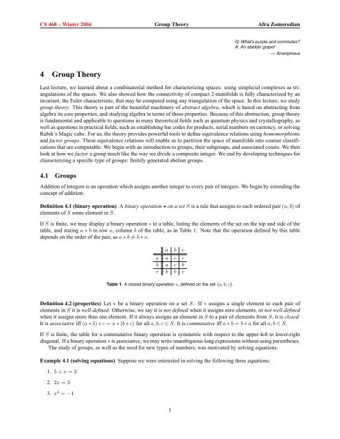
CS 468 – Winter 2004 Group Theory Afra Zomorodian
4 Group Theory
Q: What’s purple and commutes?
A: An abelian grape!
— Anonymous
Last lecture, we learned about a combinatorial method for characterizing spaces: using simplicial complexes as triangulations
of the spaces. We also showed how the connectivity of compact 2-manifolds is fully characterized by an
invariant, the Euler characteristic, that may be computed using any triangulation of the space. In this lecture, we study
group theory. This theory is part of the beautiful machinery of abstract algebra, which is based on abstracting from
algebra its core properties, and studying algebra in terms of those properties. Because of this abstraction, group theory
is fundamental and applicable to questions in many theoretical fields such as quantum physics and crystallography, as
well as questions in practical fields, such as establishing bar codes for products, serial numbers on currency, or solving
Rubik’s Magic cube. For us, the theory provides powerful tools to define equivalence relations using homomorphisms
and factor groups. These equivalence relations will enable us to partition the space of manifolds into coarser classifications
that are computable. We begin with an introduction to groups, their subgroups, and associated cosets. We then
look at how we factor a group much like the way we divide a composite integer. We end by developing techniques for
characterizing a specific type of groups: finitely generated abelian groups.
4.1 Groups
Addition of integers is an operation which assigns another integer to every pair of integers. We begin by extending the
concept of addition.
Definition 4.1 (binary operation) A binary operation ∗ on a set S is a rule that assigns to each ordered pair (a, b) of
elements of S some element in S.
If S is finite, we may display a binary operation ∗ in a table, listing the elements of the set on the top and side of the
table, and stating a ∗ b in row a, column b of the table, as in Table 1. Note that the operation defined by this table
depends on the order of the pair, as a ∗ b �= b ∗ a.
a b c
a a c c
b a c b
c b b c
Table 1. A closed binary operation ∗, defined on the set {a, b, c}.
Definition 4.2 (properties) Let ∗ be a binary operation on a set S. If ∗ assigns a single element to each pair of
elements in S it is well-defined. Otherwise, we say it is not defined when it assigns zero elements, or not well-defined
when it assigns more than one element. If it always assigns an element in S to a pair of elements from S, it is closed.
It is associative iff (a ∗ b) ∗ c = a ∗ (b ∗ c) for all a, b, c ∈ S. It is commutative iff a ∗ b = b ∗ a for all a, b ∈ S.
If S is finite, the table for a commutative binary operation is symmetric with respect to the upper-left to lower-right
diagonal. If a binary operation ∗ is associative, we may write unambiguous long expressions without using parentheses.
The study of groups, as well as the need for new types of numbers, was motivated by solving equations.
Example 4.1 (solving equations) Suppose we were interested in solving the following three equations:
1. 5 + x = 2
2. 2x = 3
3. x 2 = −1
1

CS 468 – Winter 2004 Group Theory Afra Zomorodian
The equations imply the need for negative integers Z − , rational numbers Q, and complex numbers C, respectively.
Recalling algebra from 8th grade, I solve equation (1) above, listing the properties needed at each step.
5 + x = 2 Given
−5 + (5 + x) = −5 + 2 Addition property of equality
(−5 + 5) + x = −5 + 2 Associative property of addition
0 + x = −5 + 2 Inverse property of addition
x = −5 + 2 Identity property of addition
x = −3 Addition
We take all the properties we need to solve this equation to define a group.
Definition 4.3 (group) A group 〈G, ∗〉 is a set G, together with a binary operation ∗ on G, such that the following
axioms are satisfied:
(a) ∗ is associative.
(b) ∃e ∈ G such that e ∗ x = x ∗ e = x for all x ∈ G. The element e is an identity element for ∗ on G.
(c) ∀a ∈ G, ∃a ′ ∈ G such that a ′ ∗ a = a ∗ a ′ = e. The element a ′ is an inverse of a with respect to the operation ∗.
If G is finite, the order of G is |G|. We often omit the operation and refer to G as the group.
The identity and inverses are unique in a group. We may easily show, furthermore that (a∗b) ′ = b ′ ∗a ′ , for all a, b ∈ G
in group 〈G, ∗〉.
Example 4.2 〈Z, +〉, 〈R − {0}, ·〉, 〈R, +〉, are all groups.
� Note that only one operation is allowed for groups, so we choose either multiplication or addition for integers,
for example. When we do so, the other operation is not even defined. So, do not use it!
We are mainly interested in groups with commutative binary operations.
Definition 4.4 (abelian) A group G is abelian if its binary operation ∗ is commutative.
We borrow terminology from arithmetic usually for abelian groups, using + or juxtaposition for the operation, 0 or
1 to denote identity, and −a or a −1 for inverses. It is easy to list the possible structures for small groups using the
following fact, derived from the definition of groups: each element of a finite group must appear once and only once
in each row and column of its table. Using this fact, Table 2 shows all possible structures for groups of size 2, 3, and 4
in Table 2. There are, in fact, three possible groups of size 4, but only two unique structures: we get the other one by
renaming elements.
Z2 e a
e e a
a a e
Z3 e a b
e e a b
a a b e
b b e a
Z4 0 1 2 3
0 0 1 2 3
1 1 2 3 0
2 2 3 0 1
3 3 0 1 2
Table 2. Structures for groups of size 2, 3, 4.
V4 e a b c
e e a b c
a a e c b
b b c e a
c c b a e
Example 4.3 (symmetry groups) An application of group theory is the study of symmetries of geometric figures. An
isometry is a distance-preserving transformation in a metric space. A symmetry is any isometry that leaves the object
as a whole unchanged. The symmetries of a figure form a group. A human, abstracted in Figure 1 (a) as a stick figure,
has only two symmetries: the identity, and reflection along the vertical line shown. It is immediate that a human’s
group of symmetry is Z2, as this is the only group with two elements. The letter “H” (b) has three different types of
symmetries shown: reflections along the horizontal and vertical axes, and rotation by 180 degrees. If we write down
2

CS 468 – Winter 2004 Group Theory Afra Zomorodian
(a) Humans have Z2 symmetry
a
Figure 1. Two figures and their symmetry groups.
c
(b) The letter “H” has V4 symmetry
(a) View of column (b) Motif & Design
Figure 2. Tiled Design from Masjid-e-Shah in Isfahan, Iran (a) repeats the prophet’s name (b) to obtain a figure (c) with Z4 symmetry.
the table corresponding to compositions of these symmetries, we get the group V4, one of the two groups with four
elements, as shown in Table 2.
Designers have used symmetries throughout history to decorate buildings. Figure 2 (a) shows a view of a column
of Masjid-e-Shah, a mosque in Isfahan, Iran, that was completed in 1637. The design in the center of the photo
pictorializes the name of the prophet of Islam, Mohammad as the motif in a design (b). This figure is unchanged by
rotations by multiples of 90 degrees. Letting e, a, b, c be rotations by 0, 90, 180, and 270 degrees, respectively, and
writing down the table of compositions, we get Z4, the other group with four elements in Table 2. That is, the design
has Z4 symmetry.
4.2 Subgroups and Cosets
As for sets, we may try to understand groups by examining the building blocks they are composed of. We begin by
extending the concept of a subset to groups.
Definition 4.5 (induced operation) Let 〈G, ∗〉 be a group and S ⊆ G. If S is closed under ∗, then ∗ is the induced
operation on S from G.
Definition 4.6 (subgroup) A subset H ⊆ G of group 〈G, ∗〉 is a subgroup of G if H is a group and is closed under
∗. The subgroup consisting of the identity element of G, {e} is the trivial subgroup of G. All other subgroups are
nontrivial.
We can identify subgroups easily, using the following theorem.
Theorem 4.1 H ⊆ G of a group 〈G, ∗〉 is a subgroup of G iff:
3
b
a

CS 468 – Winter 2004 Group Theory Afra Zomorodian
1. H is closed under ∗,
2. the identity e of G is in H,
3. for all a ∈ H, a −1 ∈ H.
Example 4.4 [Z4] The empty set is a trivial subgroup of any group, including Z4. The only nontrivial proper subgroup
of Z4 in Table 2 is {0, 2}. {0, 3} is not a subgroup of Z4 as 3 ∗ 3 = 2 �∈ {0, 3}, so the set is not closed under the binary
operation stated in the table. In other words, the operation is not induced in the subset.
Example 4.5 [transformations] In the first lecture, we talked about Felix Klein’s unifying definition of geometry and
topology as the study of invariant properties under transformation. We may now state his full definition. The set of
all transformations of a space forms a group under composition. A geometry is the study of those properties of a
space that remain invariant under some fixed subgroup of the full transformation group. The set of isometries forms a
subgroup of the full transformation group. The Euclidean geometry is the study of those properties left invariant under
the group of isometries. Similarly, homeomorphisms form a subgroup of the full transformation group, and topology
is the study of invariants of spaces under this subgroup.
Given a subgroup, we may partition a group into sets, all having the same size as the subgroup. The cosets are
basically like the “evil” siblings of the subgroup we use to partition the group. They look very much like the subgroup,
but are not groups themselves.
Theorem 4.2 Let H be a subgroup of G. Let the relation ∼L be defined on G by: a ∼L b iff a −1 b ∈ H. Let ∼R be
defined by: a ∼R b iff ab −1 ∈ H. Then ∼L and ∼R are both equivalence relations on G.
Note that a −1 b ∈ H ⇒ a −1 b = h ∈ H ⇒ b = ah. We use these relations to define cosets.
Definition 4.7 (cosets) Let H be a subgroup of group G. For a ∈ G, the subset aH = {ah | h ∈ H} of G is the left
coset of H containing a, and Ha = {ha | h ∈ H} is the right coset of H containing a.
For an abelian subgroup H of G, ah = ha, ∀a ∈ G, h ∈ H, so left and right cosets match. We may easily show that
every left coset and every right coset has the same size by constructing a 1-1 map of H onto a left coset gH of H for
a fixed element g of G. If a subgroup’s left and right cosets match, we say that the subgroup is normal.
Definition 4.8 (normal) A subgroup H of a group G is normal if its left and right cosets coincide, that is, if gH = Hg
for all g ∈ G.
Example 4.6 [Z4] As we saw in Example 4.4, {0, 2} is a subgroup of Z4. It is normal as Z4 is abelian. The coset of
1 is 1 + {0, 2} = {1, 3}. The cosets {0, 2} and {1, 3} exhaust all of Z4.
4.3 Factor Groups
Given a normal subgroup, we would like to treat the cosets as individual elements of a smaller group. To do so, we
first derive a binary operation from the group operation of G.
Theorem 4.3 Let H be a subgroup of a group G. Then, left coset multiplication is well-defined by the equation
(aH)(bH) = (ab)H, iff left and right cosets coincide.
We can show that this multiplication is well-defined as it does not depend on the elements a, b chosen from the cosets.
Using left coset multiplication as a binary operation, we get new groups.
Corollary 4.1 Let H be a subgroup of G whose left and right cosets coincide. Then, the cosets of H form a group
G/H under the binary operation (aH)(bH) = (ab)H.
Definition 4.9 (factor group) The group G/H in Corollary 4.1 is the factor group (or quotient group) of G modulo H.
The elements in the same coset of H are said to be congruent modulo H.
4

CS 468 – Winter 2004 Group Theory Afra Zomorodian
Example 4.7 (Factoring Z6) The cyclic group Z6, on the left, has {0, 3} as a subgroup. As Z6 is abelian, {0, 3} is
normal, so we may factor Z6 using this subgroup, getting cosets {0, 3}, {1, 4}, and {2, 5}. Figure 3 shows the table
for Z6, ordered and colored according to the cosets. The color pattern gives rise to a smaller group, shown on the
Z 6
0
3
1
4
2
5
0
0 3
3 0
1 4
4 1
2 5
5
3
2
1
1 4 2 5
4 1
2 5
5
4
2
3 0
0 3
2
5
5
2
3 0
0 3
4 1
1 4
Figure 3. Z6/{0, 3} is isomorphic to Z3.
right, where each coset is collapsed to a single element. Comparing this new group to the structures in Table 2, we
observe that it looks very much like Z3, the group of order 3. That is, the two groups are isomorphic (we formalize
this concept later in this lecture.) We write Z6/{0, 3} ∼ = Z3. Moreover, {0, 3} with binary operation +6 is isomorphic
to Z2, as one may see from the top left corner of the table for Z6. So, we have Z6/Z2 ∼ = Z3. Similarly, Z6/Z3 ∼ = Z2,
as shown in Figure 4.
Z 6 0
0
2
4
1
3
5
2 4
0 2 4
2 4 0
4 0 2
1
3
5
3 5 1
5 1 3
1 3 5
1
3
5
3 5 1
5 1 3
2 4 0
4
0 2
0 2 4
Figure 4. Z6/{0, 2, 4} is isomorphic to Z2.
� For a beginner, factor groups seem to be of the hardest concepts in group theory. Given a factor group G/H,
the key idea to remember is that each element of the factor group has the form aH: it is a set, a coset of H.
Now, we could represent each element of a factor group with a representative from the coset. For example, the element
4 could represent the coset {1, 4} for factor group Z6/{0, 3}. However, don’t forget that this element is congruent to
1 modulo {0, 3}.
4.4 Homomorphisms
Having defined groups, a natural question that arises is to characterize groups: how many “different” groups are there?
This is yet another classification problem and it is the fundamental question studied in group theory. Since we are
interested in characterizing the structure of groups, we define maps between groups to relate their structures.
Definition 4.10 (homomorphism) A map ϕ of a group G into a group G ′ is a homomorphism if ϕ(ab) = ϕ(a)ϕ(b)
for all a, b ∈ G. For any groups G and G ′ , there’s always at least one homomorphism ϕ: G → G ′ , namely the trivial
homomorphism defined by ϕ(g) = e ′ for all g ∈ G, where e ′ is the identity in G ′ .
In other words, a homomorphism is a linear map, where linearity is defined relative to the group binary operation.
Analogs of injections, surjections, and bijections exist for maps between groups. They have their own special names,
however.
5
*
*

CS 468 – Winter 2004 Group Theory Afra Zomorodian
Definition 4.11 (mono-, epi-, iso-morphism) A 1-1 homomorphism is an monomorphism. A homomorphism that is
onto is an epimorphism. A homomorphism that is 1-1 and onto is an isomorphism. We use ∼ = for isomorphisms.
Isomorphisms between groups are like homeomorphisms between topological spaces. We may use isomorphisms to
define an equivalence relationship between groups, formalizing our notion for similar structures for groups.
Theorem 4.4 Let G be any collection of groups. Then ∼ = is an equivalence relation on G.
All groups of order 4, for example, are isomorphic to one of the two 4 by 4 tables in Table 2, so the classification
problem is fully solved for that order. We need smarter techniques, however, to settle this question for higher orders.
Homomorphisms preserve the identity, inverses, and subgroups in the following formal sense.
Theorem 4.5 Let ϕ be a homomorphism of a group G into a group G ′ .
1. If e is the identity in G, then ϕ(e) is the identity e ′ in G ′ .
2. If a ∈ G, then ϕ(a −1 ) = ϕ(a) −1 .
3. If H is a subgroup of G, then ϕ(H) is a subgroup of G ′ .
4. If K ′ is a subgroup of G ′ , then ϕ −1 (K ′ ) is a subgroup of G.
Homomorphisms also define a special subgroup in their domain.
Definition 4.12 (kernel) Let ϕ : G → G ′ be a homomorphism. The subgroup ϕ −1 ({e ′ }) ⊆ G, consisting of all
elements of G mapped by ϕ into the identity e ′ of G ′ , is the kernel of ϕ, denoted by ker ϕ.
We illustrate the kernel in Figure 5. Note that ker ϕ is a subgroup by an application of the fourth statement of
Theorem 4.5 as {e ′ } is the trivial subgroup of G ′ . Since the kernel is a subgroup, we may use it to partition G into
cosets.
Theorem 4.6 Let ϕ : G → G ′ be a homomorphism, and let H = ker ϕ. Let a ∈ G. Then the set
ϕ −1 {ϕ(a)} = {x ∈ G | ϕ(x) = ϕ(a)}
is the left coset aH of H, and is also the right coset Ha of H.
The two partitions of G into left cosets and into right cosets of ker ϕ are the same, according to the theorem. That is,
the kernel is normal.
4.5 Finitely Generated Abelian Groups
We are primarily interested in finitely generated abelian groups. These groups will arise as descriptions of the connectivity
of topological spaces. To understand the structure of these groups, we utilize our usual approach: understand
simple structures first, and try to construct complicated structures from these building blocks. We begin with cyclic
groups, the simplest group there is.
G
ker ϕ
ϕ
G’
Figure 5. A homomorphism ϕ: G → G ′ and its kernel.
6
e’

CS 468 – Winter 2004 Group Theory Afra Zomorodian
Theorem 4.7 Let G be a group and let a ∈ G. Then, H = {a n | n ∈ Z} is a subgroup of G and is the smallest
subgroup of G that contains a, that is, every subgroup containing a contains H.
Definition 4.13 (cyclic group) The group H of Theorem 4.7 is the cyclic subgroup of G generated by a, and will be
denoted by 〈a〉. If 〈a〉 is finite, then the order of a is |〈a〉|. An element a of a group G generates G and is a generator
for G if 〈a〉 = G. A group G is cyclic if it has a generator.
For example, Z = 〈1〉 under addition, and is therefore cyclic. We can also define finite cyclic groups using a new
binary operation.
Definition 4.14 (modulo) Let n be a fixed positive integer and let h and k be any integers. The remainder r when
h + k is divided by n is the sum of h and k modulo n.
Definition 4.15 (Zn) The set {0, 1, 2, . . . , n − 1} is a cyclic group Zn of elements under addition modulo n.
This definition is the reason why we named the single group of order three and one of the groups of order four in
Table 2 Z3 and Z4, respectively. We may fully classify cyclic groups, using the theorem below.
Theorem 4.8 (classification of cyclic groups) Any infinite cyclic group is isomorphic to Z under addition. Any finite
cyclic group of order n is isomorphic to Zn under addition modulo n.
Consequently, we may use Z and Zn as the prototypical cyclic groups.
We next extend the idea of a generator to multiple generators for a group. Each generator generates some portion
of the elements. We put them together using intersection of groups.
Theorem 4.9 The intersection of subgroups Hi of a group G for i ∈ I is again a subgroup of G.
Let G be a group and let ai ∈ G for i ∈ I. There is at least one subgroup of G containing all the elements ai, namely
G, itself. Theorem 4.9 allows us to take the intersection of all the subgroups of G containing all ai to obtain a subgroup
H of G. Clearly, H is the smallest subgroup containing all ai.
Definition 4.16 (finitely generated) Let G be a group and let ai ∈ G for i ∈ I. The smallest subgroup of G containing
{ai | i ∈ I} is the subgroup generated by {ai | i ∈ I}. If this subgroup is all of G, then {ai | i ∈ I} generates G
and the ai are the generators of G. If there is a finite set {ai | i ∈ I} that generates G, then G is finitely generated.
Having defined what we mean by finitely generated groups, we may look at a complete description of their structure.
Theorem 4.10 (direct products) Let G1, G2, . . . , Gn be groups. For (a1, a2, . . . , an) and
(b1, b2, . . . , bn) in �n i=1 Gi, define (a1, a2, . . . , an)(b1, b2, . . . , bn) to be (a1b1, a2b2, . . . , anbn). Then �n group, the direct product of the groups Gi, under this binary operation.
i=1 Gi is a
� The definition defines its elements to be tuples made up from elements from each of the sets. It also defines its
binary operation by utilizing the binary operations of all the groups. That is, in the product of the two tuples,
aibi is the element in group Gi that the group binary operation assigns to it.
The direct product is often written with the symbol ⊗ to distinguish it from the binary operation of the group (which
may be indicated as a product.) Sometimes, it is called the direct sum, indicated by a ⊕. Although these symbols
seem to be designed to scare non-specialists away, they do help to keep the distinction between different operations
clear, especially when we have additional operations in advanced algebra. The following theorem gives a complete
characterization of the structure of finitely generated abelian groups as the direct product of cyclic groups.
Theorem 4.11 (fundamental theorem of finitely generated abelian groups) Every finitely generated abelian group
is isomorphic to product of cyclic groups of the form
Zm1
× Zm2 × . . . × Zmr × Z × Z × . . . × Z,
where mi divides mi+1 for i = 1, . . . , r − 1. The direct product is unique; that is, the number of factors of Z is unique
and the cyclic group orders mi are unique.
7

CS 468 – Winter 2004 Group Theory Afra Zomorodian
Note how the product is composed of a number of infinite and finite cyclic group factors. Intuitively, the infinite part
captures those generators that are “free” to generate as many elements as they wish. This portion of the group is a free
group that acts like a vector space. The group may be given a basis of generators from which we may generate the
group. The number of generators is called the rank of the free group. The finite or “torsion” part, on the other hand,
captures generators with finite order. This portion is like a strange vector space that does not allow us to move freely
in every dimension. In fact, this portion is called a module. We do not have enough time in this course to discuss these
structures in detail.
Definition 4.17 (Betti number, torsion) The number of factors of Z in Theorem 4.11 is the Betti number β(G) of G.
The orders of the finite cyclic groups are the torsion coefficients of G.
Example 4.8 (V4) In Table 2, we listed the binary operations for the two different groups of order four. We now
know Z4 to be the cyclic group under addition modulo four. It is already characterized in the form specified by the
fundamental theorem, so there is nothing for us to do. It is clear from the structure of V4 that it is not cyclic, that is, no
single element generates it. Otherwise, it would simply be isomorphic to Z4 by Theorem 4.8. But V4 is a finite group,
so it is finitely generated, and we should be able to characterize it according to the theorem. The only other way to
get a direct product of cyclic groups with four elements is Z2 × Z2. This group must be isomorphic to either Z4 or
V4 by our claim. By its definition, the order of each element in Z2 × Z2 is two. But Z4 has one element, namely the
generator, with order four. Therefore, Z4 � ∼ = Z2 × Z2 and it must be that V4 ∼ = Z2 × Z2. Let us check this fact by
writing the table for the binary operation of Z2 × Z2.
Z2 × Z2 (0, 0) (0, 1) (1, 0) (1, 1)
(0, 0) (0, 0) (0, 1) (1, 0) (1, 1)
(0, 1) (0, 1) (0, 0) (1, 1) (1, 0)
(1, 0) (1, 0) (1, 1) (0, 0) (0, 1)
(1, 1) (1, 1) (1, 0) (0, 1) (0, 0)
This quickly establishes an explicit isomorphism h: Z2 × Z2 → V4, where h(0, 0) = e, h(0, 1) = a, h(1, 0) = b, and
h(1, 1) = c (we have abused notation for clarity.) This group is known as the Klein Viergruppe.
4.6 Group Presentations
We end this lecture with a short and informal treatment of group presentations, a method for specifying finitely generated
groups. By the fundamental theorem, a finitely generated group has a number of free and torsional generators.
We represent each generator of the group as a unique letter in an alphabet. Any symbol of the form a n = aaaa · · · a (a
string of n ∈ Z a’s) is a syllable and a finite string of syllables is a word. The empty word 1 does not have any syllables.
We modify words naturally using elementary contractions, replacing a m a n by a m+n . Recall now that the torsional
generators have limited power: they cannot generate as many elements as they wish. We represent this limitation via
relations, equations of the form r = 1, where r is a word in our alphabet.
A presentation allows us to write all possible strings that correspond to the elements of the presented groups.
Formally, there is an isomorphism between the strings generated and the group elements. For example, the cyclic group
Z6 may be presented by a single generator a and the relation a 6 = 1. We use (a : a 6 ) for denoting this presentation.
Another presentation for Z6 is (a, b : a 2 , b 3 , aba −1 b −1 ). This presentation shows the underlying structure of Z6 as
Z2 × Z3. The last relation captures the commutativity of the group operation and is usually called the commutator.
8

CS 468 – Winter 2004 Group Theory Afra Zomorodian
Acknowledgments
Most of this lecture is from Fraleigh’s magnificent introductory book on abstract algebra [2]. Another excellent book
is Gallian [3]. For a more advanced treatment, see Dummit & Foote [1].
References
[1] DUMMIT, D., AND FOOTE, R. Abstract Algebra. John Wiley & Sons, Inc., New York, NY, 1999.
[2] FRALEIGH, J. B. A First Course in Abstract Algebra, sixth ed. Addison-Wesley, Reading, MA, 1998.
[3] GALLIAN, J. A. Contemporary Abstract Algebra, fifth ed. Houghton Mifflin College, Boston, Massachusetts, 2002.
9