Parameterization II - Computer Graphics Laboratory
Parameterization II - Computer Graphics Laboratory
Parameterization II - Computer Graphics Laboratory

You also want an ePaper? Increase the reach of your titles
YUMPU automatically turns print PDFs into web optimized ePapers that Google loves.
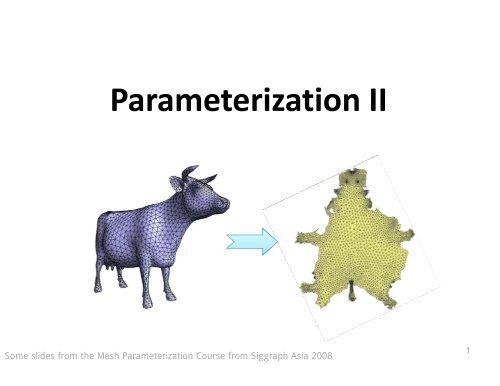
<strong>Parameterization</strong> <strong>II</strong><br />
Some slides from the Mesh <strong>Parameterization</strong> Course from Siggraph Asia 2008<br />
1
Non-Convex Non Convex Boundary<br />
• Convex boundary creates<br />
significant distortion<br />
• “Free” boundary is better<br />
2
Fixed vs Free Boundary<br />
3
Fixed vs Free Boundary<br />
4
Cut graph<br />
7
Free Boundary Methods - Tactics<br />
• Solve for the (u,v) coordinates using the discrete first<br />
fundamental form<br />
– MIPS [Hormann et al., 2000]<br />
– Stretch optimization [Sander et al., 2001]<br />
– LSCM (conformal, linear) [Levy et al., 2002]<br />
– DCP ( (conformal, f l li linear) ) [Desbrun et al., 2002]<br />
• Solve for the angles of the map (conformal)<br />
– ABF [Sheffer et al., 2001], ABF++ [Sheffer et al., 2004]<br />
– LinABF (linear) [Zayer et al., al 2007]<br />
9
Free Boundary Methods - Tactics<br />
• Solve for the edge g lengths g of the map pby yp prescribing g<br />
curvature<br />
– Circle patterns [Kharevych et al., 2006]<br />
– CPMS (linear) [ [Ben-Chen h et al., l 2008] ]<br />
– CETM [Springborn et al., 2008]<br />
• Balance area/conformality<br />
– ARAP [Liu et al., 2008]<br />
• More…<br />
10
Back to the First Fundamental Form<br />
11
Linear Map Surgery<br />
• Singular g Value Decomposition p (SVD) ( ) of<br />
with rotations and<br />
and scale factors ( (singular values) )<br />
12
Notion of Distortion<br />
• isometric or length-preserving<br />
length preserving<br />
• conformal or angle-preserving<br />
• equiareal q or area-preserving p g<br />
• everything defined pointwise on<br />
13
Computing the Stretch Factors<br />
• first fundamental form<br />
• eigenvalues of<br />
• singular values of<br />
and<br />
14
Measuring Distortion<br />
• local distortion measure<br />
• has minimum at<br />
– isometric measure<br />
– conformal measure<br />
• overall distortion<br />
15
Piecewise Linear <strong>Parameterization</strong>s<br />
• piecewise linear atomic maps<br />
• distortion constant per triangle<br />
• overall distortion<br />
16
Distortion Based Methods<br />
• Define energy functional F as a function of J Jp, I Ip, σ1,σ2 • Expand their expression in F in function of the<br />
unknown u uii, v i<br />
• Design an algorithm to find the u uii,vv i's i s that<br />
minimizes F<br />
17
Linear Methods<br />
• the terms and are quadratic<br />
in the parameter points<br />
• Dirichlet energy<br />
• Conformal energy<br />
• minimization yields linear problem<br />
[Pinkall & Polthier 1993]<br />
[Eck et al. 1995]<br />
[Lévy et al. 2002]<br />
[Desbrun [ et al. 2002] ]<br />
18
Linear Methods<br />
• both result in barycentric mappings with<br />
discrete harmonic weights for interior vertices<br />
• Dirichlet maps require to fix all boundary vertices<br />
• Conformal maps only two<br />
– result depends on this choice<br />
– best choice → [Mullen et al. 2008]<br />
• both maps not necessarily bijective<br />
19
Non-linear Non linear Methods<br />
• MIPS energy [Hormann &Greiner2000]<br />
& Greiner 2000]<br />
• Area-preserving MIPS [Degener et al. 2003]<br />
20
Non-linear Non linear Methods<br />
• Green-Lagrange Green Lagrange deformation tensor<br />
[Maillot et al al. 1993]<br />
• Stretch energies g ( , , and symmetric y stretch) )<br />
[Sander et al. 2001]<br />
[Sorkine et al. 2002]<br />
21
Conformal <strong>Parameterization</strong> - LSCM<br />
Cauchy Riemann equations:<br />
No Piecewise Linear solution in general<br />
v<br />
u<br />
⎧∂ ⎪ v ∂u<br />
⎪<br />
=−<br />
⎪ ∂ x ∂ y<br />
⎨<br />
⎪∂ ⎪ v ∂u<br />
⎪ =<br />
⎪∂ ⎪⎩<br />
∂y ∂ ∂x<br />
22
Conformal <strong>Parameterization</strong> – LSCM<br />
Minimize<br />
∑<br />
T<br />
[Levy et al., 2002]<br />
⎛ ∂ ∂v ⎞ ⎛ ∂u<br />
⎞<br />
⎟<br />
∂<br />
⎟<br />
⎜ ⎟ ⎜−⎟<br />
⎜ x⎟ ⎜<br />
y⎟<br />
⎜<br />
∂ ⎟ ⎜ ∂ ⎟<br />
⎜ ⎟−⎜ ⎟<br />
⎜∂v ⎟<br />
⎜ ⎟<br />
⎜ ⎟ ⎜ ∂ u ⎟<br />
⎜ ⎜<br />
⎜<br />
⎟ ⎟<br />
y ⎟ ⎜<br />
⎝∂⎠ ⎝⎜ ∂x<br />
⎠⎟<br />
2<br />
Fix two vertices to<br />
determine rot rot,transl,scaling<br />
transl scaling<br />
23
Conformal <strong>Parameterization</strong> - LSCM<br />
Equivalent formulation formulation, uses only edge lengths<br />
ratios and angles<br />
For each triangle: p1 p2 p − p = R<br />
α<br />
p −p<br />
2<br />
1 3 2 3<br />
l l1<br />
( ) ( ) l<br />
l 2 α<br />
p 3<br />
l 1<br />
24
x 1<br />
i<br />
Conformal <strong>Parameterization</strong> – DCP<br />
γi<br />
γ<br />
βi<br />
0<br />
x 0<br />
α<br />
[D [Desbrun b et t al., l 2002]<br />
β<br />
x 2<br />
For one triangle:<br />
90<br />
γ ( x − x ) + β(<br />
x − x ) = R ( x −x<br />
)<br />
cot cot<br />
2 0 1 0 1 2<br />
For complete one-ring of triangles<br />
(interior vertex):<br />
n<br />
(cot γ + cot β ) x − x = 0<br />
∑<br />
i=<br />
1<br />
i i i<br />
( )<br />
For incomplete one-ring of triangles<br />
(boundary vertex):<br />
n<br />
90<br />
i<br />
∑ γγi + ββi<br />
( x xi − x 0 ) = R x xi − x<br />
1 0<br />
∑<br />
1 i2<br />
i=<br />
1<br />
i2<br />
(cot cot ) ( )<br />
0<br />
25
Isotropic <strong>Parameterization</strong>s<br />
Conformal = Harmonic<br />
26
Angle Based Flattening (ABF)<br />
• Fact: Triangular 2D mesh is defined<br />
by its angles (up to similarity)<br />
• Define problem in angle space<br />
• Angle based formulation:<br />
– Di Distortion i as ffunction i of f angles l<br />
– Validity - set of angle constraints<br />
27
Constrained Constrained Minimization<br />
• Notation: β are (given) 3D angles angles. α<br />
i<br />
i are (unknown)<br />
2D angles.<br />
• Objective: minimize (relative) deviation of angles:<br />
3T<br />
∑<br />
1<br />
D ( α ) = ( α − β )<br />
i i i<br />
i =<br />
2<br />
28
Constraints<br />
• All angles are positive (linear inequalities)<br />
inequalities).<br />
• Sum of angles in each triangle is π (linear<br />
equalities).<br />
• Sum of angles around each vertex is 2π<br />
(linear equalities).<br />
• All one-rings close properly (non-linear<br />
equalities).<br />
29
Solving<br />
• Use non-linear solver (Lagrange multipliers,<br />
NNewton t method) th d) tto solve l ffor<br />
αi • Use LSCM to embed in plane based on α i<br />
30
Examples<br />
LSCM<br />
ABF<br />
31
Examples<br />
LSCM<br />
ABF<br />
32
Linear Methods<br />
uniform harmonic mean value conformal<br />
33
Linear Methods<br />
mean value conformal<br />
34
Non-Linear Non Linear Methods<br />
ABF++ circle patterns p<br />
MIPS<br />
stretch<br />
35
Non-Linear Non Linear Methods<br />
ABF++ circle patterns MIPS<br />
stretch<br />
36
LSCM [2002]<br />
ABF++ [2005]<br />
LinABF [2007]<br />
(and many more…)<br />
Circle Patterns [2006]<br />
Ricci Flow [2007]<br />
CPMS, CETM [2008]<br />
Curvature Prescription<br />
11. Cut C t mesh h to t disk di k<br />
2. Compute new angles/lengths<br />
3. Embed in plane<br />
� Discontinuities in scale
LSCM [2002]<br />
ABF++ [2005]<br />
LinABF [2007]<br />
(and many more…)<br />
Circle Patterns [2006]<br />
Ricci Flow [2007]<br />
CPMS, CETM [2008]<br />
Curvature Prescription<br />
11. Compute new angles/lengths<br />
2. Cut Mesh to disk<br />
3. Embed in plane<br />
� No discontinuities in scale
Continuous definition<br />
Scale dependent p<br />
Gaussian Curvature<br />
Gauss-Bonnet theorem: ∫ κ = 2πχ<br />
Discrete definition: κ(v) = 2π – Σα i<br />
Scale independent !<br />
Gauss-Bonnet theorem: ∑<br />
κ = 2πχ<br />
v<br />
α i<br />
κ=π/2<br />
κ ≡1/r 2
v<br />
α i<br />
Discrete Metric<br />
Triangle edge lengths (a,b,c)<br />
are the discrete metric<br />
The metric defines the angles by the cosine law<br />
The angles define the Gaussian curvature
CPMS [2008]<br />
Original edge lengths (metric)<br />
Conformal factor (per vertex)<br />
Extend φ to edge<br />
φ () t = φ t +φ<br />
(1 − t )<br />
2 3<br />
Integrate e φ on edge<br />
l l e φ �<br />
Scale to get new edge lengths = ∫<br />
1 1<br />
( t )
What Happens to the Curvature?<br />
• Continuous conformal map<br />
Curvature<br />
after map<br />
2 φ<br />
2<br />
e κ� = κ − ∇ φ<br />
Curvature<br />
before map<br />
Conformal<br />
factor
What Happens to the Curvature?<br />
• Continuous conformal mapp<br />
2φ2 e κ� = κ −∇ φ<br />
• Discrete conformal map (for small changes)<br />
κ� ≈ κ −∇<br />
• Where did the exponent go?<br />
– Discrete curvature doesn’t scale!<br />
2 φ
The Flattening Algorithm for a Topological Disk<br />
• Set target g curvature to 0 on interior vertices<br />
• Set φ to 0 on the boundary<br />
• Find φ on interior vertices by solving<br />
• Scale edge lengths to get conformal metric<br />
• Embed new edge lengths using LSCM<br />
∇<br />
2<br />
φ = κ� − κ
Some Results
Comparison with Non-Linear Non Linear Methods<br />
ABF++ circle patterns MIPS<br />
stretch CPMS<br />
46
Reducing Area Distortion<br />
• Gather Gaussian curvature into “cone cone points” points<br />
– Target curvature not 0 everywhere<br />
• First compute new edge lengths, then cut through<br />
cone points<br />
• No discontinuities in scale<br />
47
Conformal Equivalence of Triangle Meshes [2008]<br />
52
Conformal Equivalence of Triangle Meshes [2008]<br />
• Given input mesh and target curvatures curvatures, find u st s.t.<br />
– New mesh is conformally equivalent to source mesh<br />
– Target curvatures are achieved<br />
• Mi Minimize i i convex energy �� global l b l minimum i i<br />
• First optimization step equivalent to CPMS<br />
53
Conformal Equivalence of Triangle Meshes [2008]<br />
54
<strong>Parameterization</strong> - Conclusions<br />
• Many a yMANY methods et ods out tthere e e<br />
– Fixed / free boundary<br />
– Bijective / non bijective<br />
– Conformal / area preserving<br />
– Linear / non linear<br />
– First cut then embed / cone points<br />
• Best method depends on mesh<br />
– Close to disk � linear methods can work well<br />
– Require large distortion �� prefer non-linear methods<br />
58