IMPACT OF TAXES AND TRANSFERS

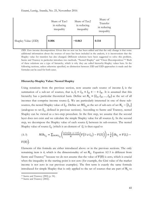
Enami, Lustig, Aranda, No. 25, November 2016
Share of Tax1
in reducing
inequality
Share of Tax2
in reducing
inequality
Share of
Transfer
in reducing
inequality
Shapley Value (ZID) 0.006 −0.063 0.114
ZID. Zero income decomposition. Given that no new tax has been added and that the only change is that some
additional information about the sources of taxes has been included in the analysis, it is inconvenient that the
Shapley value for transfers has also changed. Different solutions have been suggested to solve this problem.
Sastre and Trannoy in particular introduce two methods, “Nested Shapley” and “Owen Decomposition.” 53 Both
of these solutions use a type of hierarchy, which is why they are called hierarchy-Shapley values here. In the
following sections, unless otherwise specified, no distinction between ZID and EID approaches is made and the
formulas can be used for both cases.
Hierarchy-Shapley Value: Nested Shapley
Using notations from the previous section, now assume each source of income Ḭ i is the
summation of a sub-set of sources, that is, Ḭ i = Ḭ i1 + Ḭ i2 + ⋯ + Ḭ ik . It is assumed that this
hierarchy has a particular theoretical basis. Define set N Ii = {Ḭ i1 , Ḭ i2 , … , Ḭ ik } as the set of all
incomes that comprise income source Ḭ i . We are particularly interested in one of these subsources,
the nested Shapley value of Ḭ ij . Define set NS Iij as the set of sub-sets of set N Ii − {Ḭ ij }
(analogous to set S Ii , defined in previous sections). According to Sastre and Trannoy, nested
Shapley can be viewed as a two-step procedure. In the first step, we assume that the second
layer does not exist and we calculate the simple Shapley value for all sources Ḭ i . In the second
step, we decompose the Shapley value of each source Ḭ i between its sub-sources. The nested
Shapley value of source Ḭ ij (which is an element of Ḭ i ) is then equal to
(A-3) NSh Iij = ∑ ( (s!)×((k−s−1)!)
(V(S ∪ Ḭ ij ) − V(S))) + 1 (Sh k
I i
+ V(Ḭ i ) −
V(0)).
S∈NS Iij
k!
Elements of this formula are either introduced above or in the previous sections. The only
remaining item is k, which is the dimensionality of set N Ii . Equation A2-3 is different from
Sastre and Trannoy 54 because we do not assume that the value of V(0) is zero, which is crucial
when the inequality in the starting point is not zero (for example, the Gini value of the market
income is not zero in our previous examples). The first term is exactly the same formula
introduced for simple Shapley that is only applied to the set of sources that are part of N Ii to
53 Sastre and Trannoy (2002, p. 54).
54 Sastre and Trannoy (2002).
65