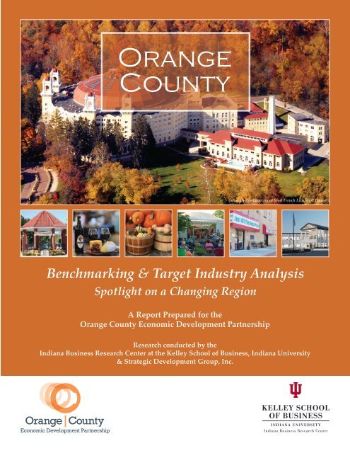
Orange County Benchmarking and Target Industry Analysis: Spotlight

Orange
County
Benchmarking & Target Industry Analysis
Spotlight on a Changing Region
A Report Prepared for the
Orange County Economic Development Partnership
Cover photos courtesy of Visit French Lick West Baden
Research conducted by the
Indiana Business Research Center at the Kelley School of Business, Indiana University
& Strategic Development Group, Inc.

Orange County
Benchmarking and
Target Industry
Analysis
Spotlight on a Changing Region
SEPTEMBER 2011
PREPARED FOR
Orange County Economic Development Partnership
RESEARCH CONDUCTED BY
� Indiana Business Research Center, Kelley School of Business, Indiana University
� Strategic Development Group, Inc.
WITH THE SUPPORT OF
� Orange County Development Commission
� Orange County REMC
� Duke Energy
� Springs Valley Bank & Trust Co.
� OCEDP

Table of Contents
EXECUTIVE SUMMARY................................................................................................................................ 2
INTRODUCTION TO THE STUDY ................................................................................................................ 5
Selection of Peer Counties ........................................................................................................................................................ 5
POPULATION AND KEY DEMOGRAPHIC CHARACTERISTICS ................................................................. 8
OC and Its Peers: Population ................................................................................................................................................. 12
EDUCATION AND EDUCATIONAL ATTAINMENT .................................................................................. 13
OC and Its Peers: Education ................................................................................................................................................... 15
INDUSTRY MIX BY EMPLOYMENT AND OCCUPATION .......................................................................... 17
OC and Its Peers: Employment Trends and GDP ............................................................................................................... 21
INCOME AND WAGES ............................................................................................................................... 24
Orange County and Its Peers: Income .................................................................................................................................. 27
COMMUTING PATTERNS .......................................................................................................................... 29
OC and Its Peers: Gross Earnings Flows .............................................................................................................................. 30
INNOVATION ............................................................................................................................................. 32
OC and Its Peers: Innovation ................................................................................................................................................. 33
HOUSING ................................................................................................................................................... 34
OC and Its Peers: Housing ..................................................................................................................................................... 36
ECONOMIC DISTRESS ............................................................................................................................... 37
OC and Its Peers: Distress Indicators .................................................................................................................................... 39
COMPARING ORANGE COUNTY AGAINST OTHER CASINO RESORT COUNTIES .............................. 41
TARGET INDUSTRY ANALYSIS ................................................................................................................ 46
Employment Base .................................................................................................................................................................... 46
Strengths and Weaknesses for New Employer Recruitment ............................................................................................. 47
Recommended Approach to New Employer Recruitment ................................................................................................ 49
Recommended Sectors to Target ........................................................................................................................................... 51
Summary................................................................................................................................................................................... 56
CONCLUSION ............................................................................................................................................ 57
APPENDIX A: METHODOLOGIES ............................................................................................................. 58
Housing Affordability Index Methodology ......................................................................................................................... 58
Innovation Index Overview ................................................................................................................................................... 58
APPENDIX B: SUPPLEMENTAL DATA ...................................................................................................... 61
APPENDIX C: SUMMARY OF 7/21/2011 EMPLOYER FOCUS GROUP ...................................................... 65
Q & A ........................................................................................................................................................................................ 65
1

Executive Summary
Nestled in south‐central Indiana, Orange County is a rural county filled with lots of natural scenery,
historical buildings, and the French Lick and West Baden Springs Hotels. Early in the 19th century,
settlers fled Orange County, NC, and its institution of slavery, thus forming the beginnings of Orange
County, IN. Covering 400 square miles, the population density remains low at 50 people per square mile.
The population has gradually grown to 19,840 residents in 2010, and the county is not expected to have a
population boom in the near future.
This study follows by five years the last major benchmarking analysis of Orange County’s economy. In
the interim, the county has experienced major improvements to the French Lick Resort, the West Baden
Springs Hotel and numerous other businesses marking a significant resurgence in the Valley area. Table
1 presents the primary indicators used in both the current and previous benchmark studies, noting
changes over the past decade and since the last report. Employment, GDP, average wage, per capita
personal income and the number of Orange County residents working within the county have
increased—all positive indicators. Unfortunately, the Great Recession (December 2007‐June 2009) likely
contributed substantially to increased rates of unemployment and poverty.
Table 1: Orange County Scorecard of Indicators
Indicator
Population
Educational Attainment
H.S. Graduate Intent to Pursue Higher Education
Total Employment
GDP
Average Wage
Per Capita Personal Income (PCPI)
Outgoing commuters
Number of Orange County residents with jobs in
Orange County
Median Home Value
Unemployment Rate
Poverty Rate
Past
Decade
Increased Decreased Little or No Change
* The data used in the 2006 and 2011 reports represent various years depending on the source.
Source: IBRC
2
Since 2006
Report *

The IBRC research team conducted a focus group with
local community leaders, and the general consensus was
that improvements had been made in the past five years,
but there is room for further improvement. Despite the
recent boost in tourism and its long history in the Valley
area, it is believed that the local tourism industry is still
in its infancy stage. Therefore, a significant portion of the
economic development focus has been centered on
businesses that would complement the existing tourism
economy. To meet this goal, it would be beneficial for
the current workforce to be trained in hospitality and
tourism management—especially for middle
management positions and future executives so existing
companies can hire from within the region.
While much attention has been given to tourism growth
in the county, manufacturing is still a large player in the
county. Despite the industry’s declining employment, employers cite the need for skilled workers with
the desire to be in manufacturing and other skilled labor positions. Transportation and logistics
challenges also exist for manufacturing companies due to the rustic transportation routes around Orange
County.
Overall, the chief challenge is improving the county’s educational attainment levels. Over the past 10
years, there has been very little change in educational attainment relative to Orange County’s peers. The
community has more high school graduates pursuing postsecondary degrees, but they are not returning
to the area. Not only does the county need to help adult workers increase their education and skills, it
also needs to entice Orange County natives to return after obtaining additional education. Local high
schools have increased their partnerships with area businesses to provide preliminary education and
training courses; however, the county would likely benefit greatly from a partnership with Ivy Tech to
provide classes for the local workforce.
Relative to its peers, Orange County remains in the middle of the pack on a number of indicators,
indicating that it is neither falling behind nor surpassing its peers. Orange County stood out in its
employment growth within the past decade—giving it the peer group’s largest share of employment in
leisure and hospitality. The mix of small and large businesses in the county helped make Orange County
the fifth most innovative county and likely contributed its fourth‐strongest GDP growth rate. In regard
to housing, Orange County has the most affordable housing market among its peers despite not having
the lowest median home value.
This report concludes with a target industry analysis conducted by Strategic Development Group (SDG),
Inc., offering guidance regarding sectors that ought to be pursued. Focusing on accommodation and
3
Overall, the chief
challenge is
improving the
county’s
educational
attainment levels.

food services growth and the existing manufacturing strength, SDG recommends the following
industries to target:
� Amusement and Theme Parks
� Continuing Care Retirement Communities
� Frozen Specialty Food Manufacturing
� Manufacturing Canned Specialty Foods
� Concrete Pipe Manufacturing
� Other Structural Clay Product Manufacturing
� Telemarketing Bureaus and Other Contact Centers
� Animal Food Manufacturing
� Plastics Packaging Materials and Unlaminated Film and Sheet Manufacturing
Compared to five years ago, community leaders feel that progress has been made—which is confirmed
by this report. While challenges still exist, the county has the ability to “re‐invent” itself—which will
require strategic planning for the future and the need to enlist the support of Orange County residents.
4

Introduction to the Study
In the fall of 2005, the Orange County Economic Development Partnership (OCEDP) asked the Indiana
Business Research Center (IBRC) at Indiana University’s Kelley School of Business to study the Orange
County economy, benchmark its performance against comparable counties and conduct a targeted
industry analysis to determine which industries the OCEDP could consider targeting in its development
efforts.
Since that study’s 2006 release, Orange County has undergone several major changes—including the re‐
opening of the French Lick Hotel and Casino as well as the West Baden Springs Hotel. Subsequently, the
OCEDP requested another study to benchmark its performance against comparable counties and
insights on industries that it could target for economic development.
By comparing Orange County to its peers, its relative strengths and weaknesses may be reviewed by
local citizens, planners and community leaders, business employees and organizations considering
where to locate or expand their operations. Moreover, by conducting such studies regularly over time, a
community can establish a basis for tracking its progress toward desired goals and for understanding
fundamental trends affecting its competitive positioning.
This report begins with a summary of how the peer counties were selected, followed by detailed analysis
of eight economic categories and the county’s performance relative to its peers and other rural casino
resort counties. These analyses are based on predominantly public data available for all the peer
counties, with additional perspective obtained via a focus group of several local community leaders. The
report concludes with discussion of potential growth industries that Orange County’s economic
development efforts could target.
Selection of Peer Counties
The IBRC selected 10 peer counties based on similarities to Orange County in the year 2000 (see Figure
1). This retroactive approach benchmarks Orange Countyʹs socioeconomic trends against communities it
was similar to recently but which may now be on divergent paths. Identifying those communities that
have prospered the most since 2000 may spur subsequent research to determine why some communities
have outperformed Orange County.
5

Figure 1: Orange County Peers
The IBRC used three steps to develop this peer set:
1. The Census Bureau’s set of 3,144 counties was limited to the 518 counties whose population
ranged from 15,000 to 25,000 residents. Analysts chose this population threshold to stay about
5,000 above and below Orange County’s 2000 population (19,306 residents).
2. The remaining counties were then compared to Orange County by their 2000 values for the
following indicators:
� Per capita personal income (PCPI)
� Percent of total employment in manufacturing
� Percent of total employment in trade and transportation
� Percent of total employment in professional services
� Percent of total employment in financial activities.
Each county’s value in the given indicators were divided by Orange Countyʹs value for that same
indicator in order to determine which county’s values were closest to Orange County’s. To
standardize these values, the absolute value of each county’s mark minus one (one represents
Orange County) was calculated. Finally, a composite score was created by summing the countyʹs
absolute values for each indicator. The lower the composite score, the more similar the county is
to Orange County with regard to these indicators. To narrow down the list, IBRC focused on the
100 lowest scores and relied on judgment to arrive at the final peer set of 10 counties. The most
6

common reason for a county with a low score to not be included was that its percent share of
manufacturing diverged too much from Orange County. Other reasons for excluding a county:
natural amenity advantages (e.g., located on or near coastline); per capita personal income less
than $28,000; excessive population loss (greater than 5 percent); and being part of a micropolitan
or metropolitan statistical area.
3. The IBRC team then consulted with OCEDP and it was determined that at least two counties
from the 2006 report should be included in the 2011 peer set to allow continuity between the two
benchmarking reports. Additionally, the 2011 report includes a brief comparison of Orange
County against seven other rural casino resort counties throughout the nation. Interestingly, one
county—Mille Lacs, MN, was included in both peer sets.
7

Population and Key Demographic
Characteristics
Orange County has gained approximately 530 new residents in the past decade, an increase of 2.8
percent. The three towns in the region each recorded population declines while the unincorporated
regions of the county grew 9.5 percent. The population increase has occurred throughout the county
with the most growth in Greenfield, Jackson and Paoli townships (see Figure 2and Table 2). The
population increase in Greenfield and Jackson townships has been dramatic—roughly 30 percent since
2000. Speculation by local leaders as to why the county is growing in its outlying townships rather than
within the towns included residents’ desires to live near, but not within, town limits due to wanting
more property, lower property values (hence lower taxes) and the lack of attractive building
opportunities within town limits.
Figure 2: Orange County Townships
Source: IBRC
Table 2: Population of Orange County Townships, Towns and Unincorporated Areas, 2000 and 2010
Census Counts
Change 2000 to
2010
2000 2010 Number Percent
Orange County 19,306 19,840 534 2.8%
French Lick Township 4,767 4,699 -68 -1.4%
French Lick Town 1,941 1,807 -134 -6.9%
West Baden Springs Town 618 574 -44 -7.1%
Balance of French Lick Township 2,208 2,318 110 5.0%
8

Census Counts
Change 2000 to
2010
2000 2010 Number Percent
Greenfield Township 559 730 171 30.6%
Jackson Township 543 686 143 26.3%
Northeast Township 578 549 -29 -5.0%
Northwest Township 345 375 30 8.7%
Orangeville Township 613 658 45 7.3%
Orleans Township 3,508 3,555 47 1.3%
Orleans Town 2,273 2,142 -131 -5.8%
Balance of Orleans Township 1,235 1,413 178 14.4%
Paoli Township 5,890 6,031 141 2.4%
Paoli Town 3,844 3,677 -167 -4.3%
Balance of Paoli Township 2,046 2,354 308 15.1%
Southeast Township 1,544 1,603 59 3.8%
Stampers Creek Township 959 954 -5 -0.5%
Source: U.S. Census Bureau
Compared to the nation and state, Orange County’s population growth has lagged in both the 1990‐2000
and the 2000‐2010 timeframes (see Figure 3). Nationally, the past decade yielded a nearly 10 percent
growth in population, but Orange County saw only a 2.8 percent increase. The state’s growth over the
past decade was at a much slower pace than its 17 percent growth between 1990 and 2000. The state’s
earlier population surge was also reflected in Orange County as it had nearly an 8 percent growth in its
population in 1990‐2000.
Figure 3: Population Growth of U.S., Indiana and Orange County, 1990‐2010
18%
16%
14%
12%
10%
8%
6%
4%
2%
0%
7.8%
Source: U.S. Census Bureau
9.7%
1990 to 2010 2000 to 2010
16.9%
6.6%
9
7.8%
2.8%
United States Indiana Orange County

Figure 4 shows the components of population change in Orange County across the past decade. Between
2003 and 2008, net migration had the most effect on population change. Net migration includes both
domestic and international migration into the county, but it is predominantly domestic migration that
drives the change. Of particular interest is the change in population in 2006 and 2007 as the French Lick
Springs Hotel was closed most of 2006 and the West Baden Springs Hotel reopened again in May 2007.
The impact of these closures/reopening can be seen by the migration decline (individuals leaving the
county) in 2006 and a subsequent uptick in 2007. Similarly, the population was also boosted by an
increase of births in 2006 and 2007. Since the reopening of the hotels, Orange County saw a decrease in
net migration in 2008 (likely due to the recession) and a slight growth in 2009 due to an increase in
births.
Figure 4: Components of Population Change, Orange County, 2000 to 2009
200
150
100
50
0
-50
-100
-150
Total Population Change Net Migration Natural Increase
2000 2001 2002 2003 2004 2005 2006 2007 2008 2009
Source: IBRC calculations based on the U.S. Census Bureau’s annual population estimates and the 2000 and 2010 decennial census counts
When looking at median age, Orange County’s residents have historically been older than the state and
that trend has continued. The county’s median age increased from 37.6 years in 2000 to 40.8 years in
2010. This compares to a 2010 median age of 37.2 years for the U.S. and 37 years for Indiana.
As shown in Figure 5, 44 percent of Orange County’s population is 45 or older. On the other end of the
spectrum, 27 percent of the population is preschool or school age (less than 20 years old). That leaves 29
percent of the population between the ages of 20 and 44. By 2020, it is projected that 45 percent of the
population will be 45 and older, 25 percent will be preschool or school age, and 30 percent will be in the
20‐to‐44 age group. The largest growth is expected to occur in the 65 and older age group, which will
increase 23 percent to comprise 19 percent of the population.
10

Figure 5: Population Distribution in Orange County, 2010
Source: U.S. Census Bureau
Overall, Orange County is not anticipated to have a major bump in total population in the near future,
but it should slowly grow at an average annual rate of 0.2 percent (see Figure 6).
Figure 6: Projected Population, 2005‐2040
21,200
21,000
20,800
20,600
20,400
20,200
20,000
19,800
19,600
19,400
19,200
28%
16%
6%
24%
21%
5%
Note: Projections are based on the 2005 population estimates.
Source: IBRC, using U.S. Census data
Preschool (0-4 years)
School Age (5 to 19 years)
College Age (20 to 24 years)
Young Adult (25 to 44 years)
Older Adult (45 to 64 years)
Older (65 plus years)
19,000
2005 2010 2015 2020 2025 2030 2035 2040
The majority of Orange County is white (97 percent), with the second‐largest racial group being black or
African‐American (0.9 percent). Another 1.2 percent of the population declared two or more races, with
half of those identifying themselves as white and American Indian/Alaska Native. The lack of diversity
in Orange County is common among the more rural counties in the state. However, in the past decade
the county has seen a 47 percent increase in its minority population.
11

OC and Its Peers: Population
Relative to its peers, Orange County has one of the smaller populations and was in the middle of the
pack regarding its average annual population growth (see Figure 7). Mille Lacs, MN, and Adams, WA,
had the highest average annual population growth rates in the past decade at 1.7 percent and 1.4 percent,
respectively. On the other end of the spectrum, Cherokee, KS, was the only peer county to post a
population loss (‐0.6 percent annually) and Lavaca, TX, did not grow at all in the past decade.
Figure 7: Population and Rate of Growth, National Peers, 2000‐2010
2010 Population
30,000
25,000
20,000
15,000
10,000
5,000
0
-5,000
Source: U.S. Census Bureau
2010 Population (left axis) Rate of Change (right axis)
12
3.0%
2.5%
2.0%
1.5%
1.0%
0.5%
0.0%
-0.5%
Averge Annual Rate of
Change, 2000 to 2010

Education and Educational
Attainment
Orange County has three school corporations serving about 3,400 students via three elementary schools
and three junior/senior high schools. The Paoli Community School Corporation serves the most students,
with roughly 1,600 students in the 2010‐2011 school year. Over the past five years, community leaders
have seen improvements made to their schools, attributed largely to the casino funds allocated to each
school in the county. Currently each student in the county receives free textbooks and the additional
funds have allowed schools to invest in building projects, additional professional development for
teachers and technology tools to further enhance the teaching environment for students. Recently, the
schools have seen improved test scores, with Springs Valley performing above the state average;
community leaders attribute this to the use of new technology tools. The local high schools also offer
$1,000 scholarships to graduating seniors who are pursuing postsecondary education via a program
initiated in 2009.
Graduation rates are an important indicator of school
success. Over the past three years, all local school
corporations have seen an increase in graduation rates.
For the 2009‐2010 academic year, the Paoli and Orleans
school corporation graduation rates exceeded the state
average of 84.1 percent, and Springs Valley School
Corporation was not far behind at 80.6 percent.
More than half of the 2010 graduating class intended to
pursue college education (60.8 percent). 1 However,
community leaders note that very few postsecondary
graduates return to Orange County, likely due to the lack of job opportunities in the area. Since 2000, the
proportion of residents with a high school diploma or less has declined only slightly. Focus group
participants speculated that the “brain drain” from the county may be reaching a turning point, noting
that more college students seem to have returned to the county in recent years.
For the majority of Orange County residents, a high school diploma or less is the highest education
attained (69.1 percent), far exceeding state and national levels (see Figure 8). Consequently, Orange
County’s proportion of individuals with at least some college is well below the state and national
averages.
1 The 2010 graduating classes’ intentions to pursue college education varies by school—Orleans: 51 percent; Paoli: 67 percent;
and Springs Valley: 72 percent.
13
Over the past three
years, all local
school corporations
have seen increased
graduation rates.

Figure 8: Educational Attainment, 2005‐2009
Note: Due to Orange County’s small population, it is necessary to use the five-year estimates.
Source: U.S. Census Bureau, American Community Survey Five-Year Estimates
The Indiana Department of Education (IDOE) collects data on graduating high school seniors and their
intent to pursue higher education degrees (see Figure 9). The IDOE reported these data by county
through 2008, but by school thereafter; thus for the 2009 and 2010 data, the IBRC research team used
current IDOE school reports to piece together the estimates. 2 In 2000 and 2001, Orange County
graduates’ intentions to pursue higher education were higher than the state average. However, in 2002,
that percentage nosedived and has remained well below the state rate. Unfortunately while the state’s
rate for postsecondary intentions has steadily increased over time, Orange County’s has been quite
volatile—likely reflecting Orange County’s small cohort relative to the state. There may be many reasons
why Orange County residents are not more interested in pursuing higher education, such as lack of
affordability and access, few employment opportunities requiring education beyond high school in the
local area and family influence (especially if parents do not have a higher education degree).
2 These data indicate only intent, not whether the students actually did attend a postsecondary institution and complete a
degree.
Bachelor's or Higher
Some College/Associate
High School or Less
United States Indiana Orange County
0 10 20 30 40 50 60 70
Percent of Population 25 or Older
14

Figure 9: Percentage of High School Graduates Intending to Pursue a Higher Education Degree, 2000‐
2010
90%
85%
80%
75%
70%
65%
60%
Indiana Orange County
2000 2001 2002 2003 2004 2005 2006 2007 2008 2009 2010
Note: Data for 2009 and 2010 were aggregated from the individual school reports.
Source: Indiana Department of Education
Regionally, county residents are able to take classes at Vincennes University (regional campus in Jasper),
at the Salem learning center, Bedford, and other locations. However, the county recognizes that it needs
county specific training in hotel and tourism management skills. Therefore, the county is involved in
ongoing dialogue with Ivy Tech about re‐opening its community learning center, thus offering higher
education courses to county residents. 3 This initiative is needed as currently the French Lick Resort has
to hire employees from outside the region to fill both upper and middle management positions, and the
resort would rather promote from within to reduce turnover and further support the community. If local
employers supported the effort, additional classes focused on workforce skills could be added to the
curriculum to address local employment needs. While it might be desirable to increase the share of
individuals with bachelor’s and above degrees, the county could benefit greatly from expanding its pool
of certificate and associate degree holders—thus the Ivy Tech partnership could be a good fit.
OC and Its Peers: Education
Among its peers, Orange County has the second‐highest percentage of individuals with a high school
diploma or less (see Table 3). Subsequently, it has the lowest percentage of individuals with some
college or associate’s degree and the second‐lowest percentage of residents with a bachelor’s degree or
higher.
Since 2000, there has been very little change in the educational attainment trends in Orange County and
McNairy County, TN, both of which have many individuals with only a high school diploma or less. The
fastest growing county in the peer group, Mille Lacs, MN, has relatively few residents with high‐school‐
or‐less attainment and the group’s highest proportion with some college or an associate degree. Research
3 Orange County had a community learning center administered by Ivy Tech, but it closed in 2010.
15

finds that individuals with certificates or associate degrees tend to stay in their hometown, whereas
those with bachelor’s degrees have a tendency to pursue occupations outside the local area. 4 Since
certificate and associate degree programs tend to be more focused on workforce preparation,
encouraging attainment of these degrees may be especially relevant for Orange County and its
employers.
Table 3: Educational Attainment Distributions, National Peers, 2000 to 2009
Bachelor’s Degree
or Higher
Some College or
Associate Degree
16
High School
or Less
2005-
2005- Change 2005- Change
2009 Change 2009 since 2009 since
National Peer Proportion since 2000 Proportion 2000 Proportion 2000
Antrim, MI 22.5% 3.1% 28.4% 0.3% 49.1% -3.4%
Putnam, GA 17.5% 3.1% 26.6% 6.1% 55.9% -9.2%
Ashe, NC 16.5% 4.4% 26.5% 3.3% 57.0% -7.7%
Cherokee, KS 14.2% 2.9% 31.3% 1.1% 54.6% -3.9%
Lavaca, TX 14.2% 2.8% 24.0% 3.5% 61.7% -6.4%
Mille Lacs, MN 13.9% 1.7% 34.0% 5.2% 52.1% -6.9%
Adams, WA 13.6% 1.4% 26.4% 1.5% 60.0% -2.9%
Seminole, OK 13.6% 1.5% 27.8% 1.5% 58.7% -2.9%
Ste. Genevieve, MO 12.2% 4.1% 25.0% 2.2% 62.9% -6.1%
Orange, IN 11.0% 0.8% 19.9% 1.5% 69.1% -2.3%
McNairy, TN 9.7% 0.9% 20.8% 1.3% 69.5% -2.2%
Note: 2000 data are from the decennial census whereas 2005-2009 data are five-year estimates which must be used due to the small population sizes.
Source: U.S. Census Bureau, American Community Survey Five-Year Estimates
4 The IBRC research team observed this pattern in the Indiana University Economic Impact Study, and recently found similar
findings among a cohort of statewide postsecondary graduates.

Industry Mix by Employment and
Occupation
Consistent with the presence of major resorts and abundant forests, Orange County’s top two industries
are accommodation‐and‐food services and manufacturing (see Table 4). 5 Together these two industries
comprised one‐third of all employment in 2009. The third‐largest employment industry is construction,
although it may be similar in size to the health care and social assistance industry (for which data are not
disclosed) that includes the IU Health–Paoli hospital and the local nursing home facilities and services.
As anticipated due to the restoration of the French Lick resorts, accommodation and food services sector
employment has surged. While manufacturing used to be the county’s major employer, its dominance
has declined over the years. As in the rest of the state and nation, manufacturing employment declined
more severely during the recession (‐11.6 percent) than during the past decade overall (‐4.9 percent
average annual rate). Other sectors that grew notably over the past decade include administrative,
support, waste management and remediation services (average annual rate of 12.8 percent); information
(4.2 percent); and real estate, rental and leasing (4.1 percent).
Table 4: Orange County Employment by Sector, 2009
2009
Employment
17
Percent
of Total
2001-2009
Average
Annual Rate
of Change
2007-2009
Average
Annual Rate
of Change
Total employment 9,446 100.0% 1.1% -1.9%
Wage and salary employment 7,908 83.7% 1.4% -2.1%
Proprietors employment 1,538 16.3% -0.5% -0.9%
Farm proprietors employment 415 4.4% -3.4% 0.0%
Nonfarm proprietors employment 1,123 11.9% 1.1% -1.3%
Farm employment 494 5.2% -2.4% -1.8%
Nonfarm employment 8,952 94.8% 1.3% -1.9%
Private employment 7,853 83.1% 1.3% -2.4%
Accommodation and food services 1,970 20.9% 23.1% -1.8%
Manufacturing 1,182 12.5% -4.9% -11.6%
Construction 945 10.0% 0.8% -0.9%
Retail trade 807 8.5% -1.9% -4.8%
Other services, except public administration 395 4.2% -0.4% -2.2%
Administrative and waste management
services
291 3.1% 12.8% 9.9%
Transportation and warehousing 212 2.2% 0.2% -7.6%
5 The majority of Orange County’s manufacturing is in the wood‐products and furniture‐related categories.

2009
Employment
18
Percent
of Total
2001-2009
Average
Annual Rate
of Change
2007-2009
Average
Annual Rate
of Change
Arts, entertainment, and recreation 196 2.1% 2.9% 9.0%
Real estate and rental and leasing 190 2.0% 4.1% -1.5%
Finance and insurance 163 1.7% 1.0% 2.9%
Information 64 0.7% 4.2% 9.3%
Forestry, fishing, and related activities ND - - -
Mining ND - - -
Utilities ND - - -
Wholesale trade ND - - -
Professional, scientific, and technical
services
ND - - -
Management of companies and enterprises ND - - -
Educational services (private only) ND - - -
Health care and social assistance ND - - -
Government and government enterprises 1,099 11.6% 1.9% 2.4%
Federal, civilian 48 0.5% -0.5% 0.0%
Military 66 0.7% 0.0% 4.1%
State and local 985 10.4% 2.2% 2.4%
State government 123 1.3% 2.1% 0.8%
Local government 862 9.1% 2.2% 2.7%
Note: ND represents non-disclosable data. This accounts for roughly 1,438 employees or 15.2 percent of total employment. Employment figures include both
payroll employees and the self-employed.
Source: Bureau of Economic Analysis
As a whole, Orange County has only a handful of declining industries—manufacturing, retail trade,
other services (excluding public administration) and farming. Total employment grew by an average of
1.1 percent annually since 2001 (94 jobs a year), largely from wage‐and‐salary employees and non‐farm
proprietors, not farm proprietors. Indeed, farm employment for both proprietors and employees
declined in the county. The Great Recession certainly impacted the county with a 3.7 percent
employment decline between 2007 and 2009. While the overall uptick in employment over the decade is
positive news, it is not enough growth to employ graduating seniors of local high schools and
postsecondary institutions.
Recognizing the county’s strength in the accommodation and food services sector, community leaders
are focusing on its tourism cluster—attracting and developing businesses that complement the resort
and casino business. Unfortunately, Orange County is not always an easy sell to outside investors due to
limited available developable land (particularly in the French Lick–West Baden area) despite the area’s
low‐cost, central location for regional markets and abundance of low‐to‐moderately‐skilled labor.
Location quotients (LQs) are widely used to show which industries have a particularly strong presence
in a region. In this study, LQs were calculated by dividing a given industry cluster’s share of total

employment in Orange County by the cluster’s corresponding share in the nation as a whole; an LQ
greater than 1 indicates that the industry cluster is more concentrated locally than the national average. 6
Table 5 shows that Orange County’s only notable strong industrial presence is in the forest and wood
products industry—more than six times greater than the national concentration. However, the LQ has
shrunk by about one‐third since 2001, showing that this cluster is losing ground relative to other parts of
the nation, even though it’s still represented far above average in the local economy. Two clusters—
chemicals and chemical‐based products and glass and ceramics—have increased their concentrations
since 2001 and pay wages below the average for all clusters. The two highest‐paying industry clusters
(life sciences and defense and security) both have low LQs, but any growth in these clusters could help
improve Orange County’s average wage.
Several clusters are not listed due to data suppression in 2009, including advanced materials;
agribusiness, food processing and technology; apparel and textiles; manufacturing; mining; and printing
and publishing.
Table 5: Orange County Industry Cluster Location Quotients and Average Wage per Job, 2001 to 2009
2001 2009 2009
Industry Cluster
LQ LQ Average Wage
Total, All Industries 1.00 1.00 $28,526
Arts, Entertainment, Recreation and Visitor
Industries
ND 0.56 $10,063
Biomedical/Biotechnical (Life Sciences) ND 0.35 $42,632
Business and Financial Services 0.08 0.07 $30,025
Chemicals and Chemical Based Products 0.10 0.16 $26,112
Defense and Security ND 0.39 $44,253
Education and Knowledge Creation 0.85 0.82 $31,390
Energy (Fossil and Renewable) 0.44 0.30 $21,971
Forest and Wood Products 9.88 6.56 $31,169
Glass and Ceramics 0.44 0.74 $26,112
Information Technology and Telecommunications 0.10 0.05 $37,446
Note: ND represents non-disclosable data.
Source: U.S. Bureau of Labor Statistics, Quarterly Census of Employment & Wages (QCEW) and Purdue Center for Regional Development (cluster definitions)
Another approach to assessing a region’s workforce strengths uses the knowledge and skills needed to
carry out a job to define occupation (rather than industry) clusters. Occupation clusters are formed by
grouping occupations with similar job functions, knowledge requirements, essential experience and the
amount of on‐the‐job training needed to accomplish the work. 7 Occupations are classified in the O*NET
6 The industry cluster data are derived from work done by the Purdue Center for Regional Development in collaboration with
the IBRC for an Economic Development Administration project titled, Unlocking Rural Competitiveness: The Role of Regional
Clusters. More information about the clusters and related work can be found at www.statsamerica.org/innovation/reports.html.
7 More information about occupation clusters and the methodology underlying them can be found at
www.statsamerica.org/innovation/reports/sections2/3.pdf.
19

system (sponsored by the U.S. Department of Labor) into five “job zones.” Job zones 1 and 2 are
characterized by relatively low skill levels, formal education requirements and wages, the likelihood of
few benefits and easy transfer between jobs. 8 The remaining zones—3 through 5—require significantly
more knowledge, skills and education. Occupations in these higher‐level zones are allocated into 15
knowledge clusters, with health care and medical science further disaggregated into three sub‐clusters.
The largest share of Orange County
workers (38 percent) fall into job zone 2
Nearly 60 percent of Orange followed by job zone 1 at 21.5 percent
(see Table 6). This means that nearly 60
County’s workforce is in percent of Orange County’s workforce is
in low‐skilled occupations requiring no
low‐skilled occupations formal training or very little training—
which may partially explain why
requiring little or no formal educational attainment is relatively low
in the county. Compared to the state,
training.
Orange County has a larger share of
low‐skilled occupations, particularly in
job zone 1. Among higher‐skilled
occupations, skilled production workers comprise the highest share of Orange County workers at 10.3
percent. Comparing the proportion of workers in select clusters to the state, Orange County has higher
proportions of its workforce in skilled production occupations and in agribusiness and food technology
jobs.
Over time, the proportion of Orange County workers in each occupation cluster has changed very little.
The most notable increase since 2001 has been a 2.2 percentage point increase in the proportion of job
zone 1 workers. The largest decreases in proportion of workers in a particular occupation cluster include
agribusiness and technology (‐1.9 percent), job zone 2 (‐0.9 percent), and skilled production workers (‐0.8
percent). The declines in job zone two and skilled production workers concern local employers that are
having difficulties finding qualified workers for hire. This is a situation where the county’s partnership
with Ivy Tech could assist the local workforce to advance from job zone one to more‐skilled labor. In
particular, employers have noticed that middle‐aged workers need more computer skills to adapt to
technological changes in the workforce.
8 O*Net definitions of job zones can be found at www.onetonline.org/help/online/zones.
20

Table 6: Occupation Cluster Mix of Orange County and Indiana, 2009
Occupation Cluster
Orange County Indiana
Employment Share Employment Share
Job Zone 2 3,533 37.9% 1,311,736 37.4%
Job Zone 1 2,002 21.5% 536,823 15.3%
Skilled Production Workers: Technicians,
Operators, Trades, Installers & Repairers
962 10.3% 304,726 8.7%
Agribusiness and Food Technology 460 4.9% 65,742 1.9%
Health Care and Medical Science
(Aggregate)
Primary/Secondary and Vocational
Education, Remediation & Social Services
440 4.7% 205,321 5.9%
433 4.6% 179,528 5.1%
Managerial, Sales, Marketing and HR 428 4.6% 249,783 7.1%
Legal and Financial Services, and Real
Estate
Health Care and Medical Science (Therapy,
Counseling and Rehabilitation )
417 4.5% 245,568 7.0%
283 3.0% 117,645 3.4%
Personal Services Occupations 126 1.4% 69,283 2.0%
Health Care and Medical Science (Medical
Technicians)
Arts, Entertainment, Publishing and
Broadcasting
Mathematics, Statistics, Data and
Accounting
Health Care and Medical Science (Medical
Practitioners and Scientists)
91 1.0% 44,938 1.3%
84 0.9% 61,209 1.8%
83 0.9% 64,344 1.8%
65 0.7% 42,738 1.2%
Public Safety and Domestic Security 61 0.7% 37,287 1.1%
Engineering and Related Sciences 56 0.6% 32,838 0.9%
Information Technology 50 0.5% 51,802 1.5%
Postsecondary Education and Knowledge
Creation
Building, Landscape and Construction
Design
Natural Sciences and Environmental
Management
45 0.5% 43,883 1.3%
26 0.3% 12,795 0.4%
10 0.1% 10,603 0.3%
Note: Job zone 1 includes occupations that need little or no preparation—the occupations may require a high school diploma or GED certificate. Some may require
a formal training course to obtain a license. Job zone 2 includes occupations that need some preparation—the occupations usually require a high school diploma
and may require some vocational training or job-related course work. In some cases, an associate or bachelor’s degree could be needed.
Source: Statsamerica.org; Economic Modeling Specialists, Inc. Complete Employment Statistics
OC and Its Peers: Employment Trends and GDP
Over the past decade, Orange County has posted an average annual employment gain of 1.1 percent,
ranking it second among its peers for employment growth (see Figure 10). Putnam, GA, led the peer set
with 1.9 percent average annual growth, while the remaining counties with positive growth grew at less
21

than 0.5 percent annually. The recession severely impacted several counties, especially McNairy, TN,
and Mille Lacs, MN. Compared to its peers, Orange County had the sixth‐highest average annual change
in employment at ‐1.9 percent between 2007 and 2009.
Figure 10: Average Annual Employment Change, National Peers, 2001 to 2009 and 2007 to 2009
2007-2009 2001-2009
-10% -8% -6% -4% -2% 0% 2%
Source: Bureau of Economic Analysis
Manufacturing and leisure & hospitality are Orange County’s top‐employing industries, so it is
instructive to compare their relative importance in the peer counties (see Figure 11). As of 2009, Ste.
Genevieve, MO, had the highest share of manufacturing jobs. Orange County had the highest share of
leisure and hospitality employment, which also experienced strong growth. (Note that leisure and
hospitality data for Adams, WA, and McNairy, TN, were non‐disclosable.) Adams County, WA, was the
only county to experience positive growth in manufacturing since 2001, and McNairy County, TN, had
the largest decline in manufacturing share. Throughout this time period, all peer counties experienced
positive growth in the leisure and hospitality industry except for Seminole, Antrim and Mille Lacs.
22
McNairy, TN
Cherokee, KS
Adams, WA
Mille Lacs, MN
Seminole, OK
Antrim, MI
Ashe, NC
Ste. Genevieve, MO
Lavaca, TX
Orange, IN
Putnam, GA

Figure 11: Share of Manufacturing and Leisure and Hospitality Employment and Trends, National
Peers, 2001 to 2009
Note: Leisure and hospitality data for McNairy and Adams counties were non-disclosable. Leisure and hospitality employment includes two industry sectors: arts,
entertainment and recreation and accommodation and food services. Change is reflected as the difference in the industry share of employment in 2009 versus
2001.
Source: Bureau of Economic Analysis
The mix of industries in a given region affects the region’s gross domestic product (GDP, its economic
output). All of the peer counties experienced increased GDP between 2000 and 2008. Of all the counties,
Ashe, NC, had the largest GDP at $856 million, whereas Antrim, MI, had the smallest at $507.5 million
(see Figure 12). Seminole, OK, has had the strongest average annual GDP growth at 8.7 percent, followed
by Lavaca, TX, at 8.5 percent. Orange County’s GDP grew at 4.2 percent annually—making it the fourth‐
fastest growing county in the peer group.
Figure 12: Estimated GDP, National Peers, 2000‐2008
GDP Value (in millions)
25%
20%
15%
10%
5%
0%
-5%
-10%
-15%
-20%
-25%
$1,000
$800
$600
$400
$200
$-
Share of Manufacturing (left axis) Share of Leisure and Hospitality (left axis)
Manufacturing Change (right axis) Leisure and Hospitality Change (right axis)
Note: 2008 is the most recent year for which GDP data are available.
Source: Moody’s Analytics
2008 GDP (left axis) Rate of Change (right axis)
23
10%
8%
6%
4%
2%
0%
Average Annual Rate of
Change, 2000-2008
15%
12%
9%
6%
3%
0%
-3%
-6%
-9%
-12%
-15%

Income and Wages
In 2010, the Orange County average wage for all
industries was $29,134—approximately $10,000 less
than the state’s average wage and $17,600 less than
the nation (see Figure 13). Orange County’s average
wage has grown about 3 percent annually over the
past decade, besting the state’s rate of 2.7 percent
and matching the national rate of wage growth. U.S.
and Orange County average wage growth has
exceeded the average rate of inflation, whereas
Indiana’s average wage has simply kept pace with
inflation in the past decade.
Figure 13: Average Wage, U.S., Indiana and Orange County, 2000 to 2010
$50,000
$45,000
$40,000
$35,000
$30,000
$25,000
$20,000
Source: Bureau of Labor Statistics
U.S. Indiana Orange County
2000 2001 2002 2003 2004 2005 2006 2007 2008 2009 2010
Table 7 shows that three industries pay higher wages in Orange County than their statewide averages—
transportation and warehousing; administration, support, waste management and remediation services;
and accommodation and food services. On the other end of the spectrum, three industries pay less than
half of the state’s average wage—arts, entertainment and recreation; management of companies and
enterprises; and real estate, rental and leasing. Unfortunately, the industries paying higher than state
average wages cover only 13.5 percent of the workforce, explaining why the county’s average wage is
slightly less than three‐fourths the state average.
24
Orange County
average wage growth
has outpaced inflation.

Table 7: Average Wage Distribution, Orange County, 2010
Average Wage
Percent of Indiana’s
Average Wage
Total Employment $29,134 74.2%
Construction $48,725 98.5%
Professional, Scientific, and Technical Services $40,967 74.8%
Transportation & Warehousing $40,404 101.8%
Manufacturing $34,069 62.6%
Finance and Insurance $32,011 59.0%
Educational Services $31,632 85.6%
Management of Companies and Enterprises $31,008 40.6%
Admin. & Support & Waste Mgt. & Rem. Services $29,333 110.4%
Public Administration $28,751 70.7%
Information $22,841 51.3%
Accommodation and Food Services $21,747 162.6%
Retail Trade $20,002 85.1%
Other Services (Except Public Administration) $18,106 69.2%
Real Estate and Rental and Leasing $15,539 45.7%
Arts, Entertainment, and Recreation $11,512 39.2%
Note: The following industries are non-disclosable: agriculture, forestry, fishing and hunting; mining; utilities; wholesale trade; and health care and social services.
Source: Bureau of Labor Statistics
Per capita personal income (PCPI) is a broader indicator of a region’s income level because it includes
many sources of income, not just wages. It includes wages/salaries, any supplements to wages and
salaries (e.g., bonuses), proprietors’ income, investment income and personal current transfer receipts,
but not contributions for government social insurance. Figure 14 shows that in 1970, the county, state
and nation were very similar in PCPI, but Orange County PCPI subsequently accelerated more slowly
than the U.S. and Indiana. Between 2006 and 2008, Orange County steadily narrowed the gap with the
state, but it still lags Indiana by roughly $5,000 and the nation by $10,000.
As of 2009, Orange County PCPI was $29,042, Indiana’s was $34,022 and U.S. PCPI was $39,635. Orange
County’s PCPI was 85.4 percent of Indiana’s PCPI and 73.3 percent of the nation’s PCPI, and it has
grown at an average annual rate of 1.1 percent over the past nine years.
25

Figure 14: Per Capita Personal Income of Orange County, Indiana and the U.S., 1970 to 2009
$45,000
$40,000
$35,000
$30,000
$25,000
$20,000
$15,000
$10,000
$5,000
$-
Source: Bureau of Economic Analysis
Indiana Orange United States
To better understand the composition of personal income, Table 8 breaks down the components
comprising the bulk of personal income. Orange County is fairly similar to the state and nation in all
categories except personal current transfer receipts.
� Net earnings by place of residence (which includes wages earned at the workplace adjusted for
government and social insurance contributions and residence) comprises the largest share of
personal income. Wages and salaries are the primary component of net earnings, followed by
supplements to wages and salaries (i.e., employer contributions to employee pension and
insurance funds and for government social insurance).
� The smallest major category of income for all areas was dividends, interest and rent, comprising
less than one‐fifth of each area’s personal income.
� The remainder of personal income is derived from personal current transfer receipts, which are
government payments to individuals for which no services are performed. Consistent with local
community leaders’ intuitions, Orange County residents are more dependent on such
government payments than are residents of the state and nation, primarily for medical benefits
and retirement and disability insurance benefits (43.7 and 35.3 percent of current transfer
receipts, respectively). The 27.8 percent of personal income coming from government payments
might help explain recurring themes in the area such as the receipt of free or subsidized lunches
in the county schools (51 percent in 2010), common perceptions that local citizens want “hand‐
outs,” and the categorization of the county as being one of the poorest in the state.
26

Table 8: Composition of Personal Income, U.S., Indiana and Orange County, 2009
Personal Income Component U.S. IN
Orange
County
Net earnings by place of residence 64.5% 65.5% 59.6%
Net earnings by place of work 72.4% 71.7% 57.9%
Wage and salary disbursements 71.1% 71.2% 73.5%
Supplements to wages and salaries 17.3% 18.2% 17.5%
Proprietors' income 11.6% 10.6% 9.1%
Dividends, interest, and rent 18.0% 14.6% 12.7%
Personal current transfer receipts 17.5% 19.9% 27.8%
Source: Bureau of Economic Analysis
Orange County and Its Peers: Income
Among the national peers, Ste. Genevieve, MO, had the highest 2010 average wage at $36,011, which is
$10,700 below the national average (see Figure 15). Overall, average wages in the peer counties averaged
around $30,300—with Antrim, MI, reporting the lowest average wage of $27,322. Orange County places
in the middle of the pack for both average wage and average annual growth rate. Six counties had faster
growth rates than the United States, led by Seminole, OK, at 7.1 percent.
Figure 15: Average Wage, National Peers, 2000 to 2010
2010 Average Wage
$50,000
$40,000
$30,000
$20,000
$10,000
$-
Source: Bureau of Labor Statistics
2010 Average Wage (left axis) Rate of Change (right axis)
Despite Ste. Genevieve having the highest average wage among the national peers, Lavaca, TX, and
Putnam, GA, recorded higher PCPIs than Ste. Genevieve (see Figure 16). This indicates that residents in
those areas obtain significant income from sources other than wages. Relative to the U.S., the national
peers’ PCPIs range from 92.7 percent (Lavaca, TX) to 65.7 percent (McNairy, TN). Orange County is in
the lower half of the peer counties for PCPI, PCPI growth rate and PCPI as a percentage of the U.S value.
27
10%
8%
6%
4%
2%
0%
Average Annual Rate of
Growth, 2000 to 2010

Figure 16: Per Capita Personal Income of National Peers, 2000 to 2009
2009 Per Capita Personal
Income (PCPI)
$45,000
$40,000
$35,000
$30,000
$25,000
$20,000
$15,000
$10,000
$5,000
$-
Source: Bureau of Economic Analysis
2009 PCPI (left axis) Rate of Change (right axis)
28
9%
8%
7%
6%
5%
4%
3%
2%
1%
0%
Average Annual Rate of
Change, 2000 to 2009

Commuting Patterns
The availability of quality jobs in other regions and the willingness of workers to travel have caused
commuting to become a way of life for many workers. The economic effects of commuting reach beyond
the individual worker to the broader community. Therefore, this study examines the commuting
patterns of workers as well as the gross earnings flows to and from counties. The available commuting
data are at the county level, with Indiana’s data being the most comprehensive.
Figure 17 shows that Lawrence and Orange County are the major sources of workers commuting into
each other’s county. Sixty‐one percent of Orange County’s inbound commuters come from Lawrence,
Washington, Dubois, Crawford and Martin counties. The commuters leaving Orange County go mainly
to either Lawrence or Dubois County with the remainder traveling to Washington, Monroe and
Kentucky. These top five counties capture 67.4 percent of all outgoing commuters.
Figure 17: Workers Commuting Into and Out of Orange County, 2009
Source: STATS Indiana Commuting Profiles, using Indiana Department of Revenue data
In 2000, 79.9 of Orange County workers were employed in the county, but by 2009 this percentage had
increased to 82.8 percent. This increase in non‐commuting residents cannot be explained solely by
growth in the implied resident labor force (individuals who live in Orange County and work), which
rose only 0.3 percent over the past nine years (see Table 9). Rather the increase primarily came from a
reduction in residents commuting out of the county. Nearly 70 percent of the county’s increase in
employment results from reduced outbound commuting and growth in the resident labor force. The
remaining 30 percent came from an increase in incoming commuters.
Commuting affects where paychecks wind up. That is, a resident who crosses county lines to work
brings her earnings home to her county of residence from the county of employment. Orange County’s
increased volume of incoming commuters thus resulted in higher gross earnings outflows. These
29

incoming commuters apparently
held higher‐paying jobs because
the gross earnings outflow
growth was more than double
the incoming commuter growth.
Meanwhile, because more
Orange County residents
secured jobs within the county, between 2000 and 2009.
the number of residents
commuting out of Orange
County declined by 14.2 percent between 2000 and 2009. Meanwhile, the gross earnings inflows
increased—which may indicate that the 2009 outbound commuters had higher paying jobs relative to the
2000 outbound commuters.
Table 9: Commuting Trends, Orange County, 2000 and 2009
The number of residents
commuting out of Orange
County declined by 14.2 percent
30
2000 2009 Change
Number Who Live in OC and Work (implied resident labor force) 12,380 12,415 0.3%
Number Who Work in OC (implied workforce) 11,315 11,873 4.9%
Number Who Live and Work in OC 9,887 10,276 3.9%
Number Who Live in OC but Work Elsewhere 2,493 2,139 -14.2%
Number Who Live Elsewhere but Work in OC 1,428 1,597 11.8%
Total Gross Earnings Inflows (in thousands of dollars) $97,080 $108,478 11.7%
Total Gross Earnings Outflows (in thousands of dollars) $44,522 $57,434 29.0%
Source: STATS Indiana Commuting Profiles, using Indiana Department of Revenue data; Bureau of Economic Analysis
OC and Its Peers: Gross Earnings Flows
Compared to its peers, Orange County has one of the lowest gross earnings inflows and the fifth‐highest
gross earnings outflow (see Figure 18). Of all the counties, nearly all have a greater value of inflows than
outflows, reflecting that either a larger portion of the workforce commutes out of the county or these
workers are able to secure higher paying positions out of the county in which they live. In all counties
(except in Antrim and McNairy), the value of inflows and outflows has risen over the past nine years.
Adams, WA, is the only county that has more gross earnings outflows than inflows, which may be due
to the increase in manufacturing occupations that was noted earlier in the report.

Figure 18: 2009 Gross Earnings Flows for National Peers, and Change since 2000
Value of Gross Earnings Flows
in 2009 (Thousands)
$200,000
$160,000
$120,000
$80,000
$40,000
$-
$(40,000)
$(80,000)
Source: Bureau of Economic Analysis
Inflows of earnings (left axis) Outflows of earnings (left axis)
Change in inflows (right axis) Change in outflows (right axis)
31
10%
8%
6%
4%
2%
0%
-2%
-4%
Average Annual Rate of
Change, 2000 to 2009

Innovation
Innovation is a widely recognized driver of economic growth. IBRC researchers have developed a
county‐level Innovation Index, which is a composite of many variables that measure both the inputs to
innovation as well as its outputs. 9 The inputs, which can be thought of as the local capacity for
innovation, include measures such as venture capital, broadband penetration, investments in R&D and
educational attainment. The inputs are divided into human capital and economic dynamics sub‐indices.
Outputs include measures considered to be byproducts of innovative economies such as employment
growth in high‐tech firms, growth in output per worker and creation of patents. The outputs are divided
into two sub‐indices—productivity & employment and economic well‐being. An Innovation Index score
of 100 indicates that an area is, on average, as innovative as the nation. The same applies to each of the
sub‐indices that comprise the overall index. 10
Orange County is very similar to Indiana in terms of innovation sub‐index scores, except for human
capital (see Figure 19). In fact, the county does slightly better than the state in economic dynamics and
economic well‐being, though none surpasses the U.S. benchmark of 100. Orange County performs well
in the economic dynamics category due to its shares of both large and small businesses. Despite Orange
County performing worse than the state in terms of poverty, unemployment and net migration, it
outscored Indiana on the economic well‐being sub‐index due to higher growth of PCPI and earnings.
Orange County’s weakest innovation sub‐index, human capital, reflects the low postsecondary
educational attainment rates in addition to a lack of high‐tech employment.
Figure 19: Innovation Index Scores, Orange County and Indiana
100
80
60
40
20
0
57.9
88.2
Source: Indiana Business Research Center
82.9
Orange County Indiana
78.9
9 A report introducing the Innovation Index, Crossing the Next Frontier: Information and Analytics Linking Regional Competitiveness
to Investment in a Knowledge‐Based Economy, and the index data may be accessed at www.statsamerica.org/innovation/.
10 See Appendix A for a more detailed description of the Innovation Index.
32
77.2
82.1
Human Capital Economic Dynamics Productivity and
Employment
98.9
97.4
Economic Well-Being

OC and Its Peers: Innovation
None of Orange County’s national peers had an Innovation Index score greater than the U.S. average of
100. Their innovation scores are relatively similar, with only a 10‐point spread between the most and
least innovative county (see Table 10). No one county performed the best across all sub‐indexes, yet all
counties had their top score in the economic well‐being category. Unfortunately, the human capital
category tended to be the sub‐index that undermined their innovation capacity (except for Ashe and
Antrim counties).
Table 10: Innovation Index Scores of National Peers
Innovation Human Economic Productivity and Economic
National Peer
Index Capital Dynamics Employment Well-Being
McNairy, TN 81.1 70.2 84.8 83.3 96.0
Mille Lacs, MN 81.1 76.4 89.3 72.6 96.2
Antrim, MI 77.1 82.0 77.4 67.4 90.6
Ashe, NC 76.5 86.6 64.1 72.5 95.4
Orange, IN 75.3 57.9 82.9 77.2 98.9
Lavaca, TX 74.4 59.1 70.8 81.5 110.3
Seminole, OK 74.4 69.3 68.6 73.1 110.8
Putnam, GA 74.1 59.9 85.2 69.2 98.3
Ste. Genevieve, MO 74.1 56.8 77.5 78.6 102.4
Adams, WA 73.3 63.5 68.8 79.7 97.1
Cherokee, KS 71.0 68.8 61.0 71.6 105.7
Note: Bold cells reflect the highest score for the sub-index category
Source: Indiana Business Research Center
33

Housing
Eighty‐six percent of Orange County’s 9,176 housing units were occupied in 2010. Both the number of
housing units and the share of vacant homes have increased (9.9 percent and 79.4 percent, respectively)
since 2000, with Orange County’s vacant‐home growth rate far above the state rate of 49.7 percent.
Three‐fourths of the occupied homes were owner‐occupied in 2010, housing 76 percent of the
population. Of the vacant homes, most are for seasonal/recreational use (33 percent), 30 percent are for
sale or rent, and the remainder are vacant for other reasons. As noted by a local real estate agent, the
number of seasonal and vacation homes has increased in the past several years; in 2000, only 18.4 percent
of vacant homes were for this use. Where the increase in vacant homes has led to blight, some
communities have initiated efforts to purchase and tear down abandoned homes in an effort to clean‐up
the aesthetic appeal of the area.
Of the 7,872 households in Orange County, 68.8 percent are family households. The majority (53.5
percent) of all households are headed by married couples, and 20 percent of married couples in the
county have children under 18 living in them. Nearly 9 percent of the homes with children under 18 are
headed by a single parent. Roughly 27 percent of households have residents living alone, with 43 percent
of those individuals age 65 or older (70 percent of which are women). As the population continues to age
in Orange County, there is a need for retirement communities to provide options for the elderly seeking
to downsize or needing assisted living.
The national housing crash that began in late 2007 did not impact Orange County like it did other
regions in the United States. In fact, the county seemed relatively sheltered from the crash, save for
reductions in sale prices, until 2009 when homes sales began to drop. Between 2005 and 2010, 185 homes
sold for an average price of $74,700. Statewide, homes sold at an average of $109,800. Despite the
significantly lower home sales price in Orange County than statewide, local community leaders noted
the need for more single‐family housing as well as for subsidized housing, and steps have been taken to
address this issue through future housing development plans.
Foreclosures are also impacting Orange County’s housing market. Figure 20 shows that Orange County
had 3.5 percent of its prime mortgages in foreclosure as of November 2010, a rate only slightly higher
than the state (3.4 percent) and nation (3.1 percent). Of Orange County’s prime mortgages in foreclosure,
most are delinquent by 30 to 59 days, followed by more than90 days (5.3 and 4.6 percent, respectively).
All of Orange County’s delinquency rates exceed the state and national figures, which could indicate a
potential for increased foreclosure rates in the county relative to the state and nation in the near future.
34

Figure 20: Comparison of Foreclosure Rates, U.S., Indiana and Orange County, November 2010
Share of Prime Mortgages in
Delinquency
Note: This database includes mortgages from nine of the top 10 mortgage servicers and represents approximately 50-70 percent of the number of mortgages in
the United States. Coverage may vary by type of mortgage and by geography. Therefore, the percentages here are likely indicative of market conditions.
Source: Federal Reserve Bank of New York
New home construction in Orange County has been volatile over the past decade (see Figure 21),
peaking in 2006 with 40 permits filed. Most of the permits have been for single‐family units, although
multi‐family permits were filed in Orange County in 1999, 2006, 2008 and 2009, as represented by the
spikes in the number of permits issued.
Figure 21: Number and Value of Permit Units, Orange County, 1999 to 2010
Number of Permit Units
45
40
35
30
25
20
15
10
5
0
6%
3%
0%
Source: U.S. Census Bureau
30-59 days delinquent 60-89 days delinquent
90+ days delinquent In foreclosure (right axis)
United States Indiana Orange, IN
Total Permits Filed (left axis) Total Permits' Cost (right axis)
1999 2000 2001 2002 2003 2004 2005 2006 2007 2008 2009 2010
35
$-
4%
2%
0%
$500
Percent in Foreclosure
$4,500
$4,000
$3,500
$3,000
$2,500
$2,000
$1,500
$1,000
Value of Permits

OC and Its Peers: Housing
Among its peers, Orange County has one of the lower median home values at $89,300—a far cry from
the $172,400 median value in Mille Lacs, MN. Taking into account the typical incomes in a given area
makes the median home value much more meaningful in terms of affordability. Moody’s Economy.com
combines these factors in its single‐family housing affordability index—a measure based on an area’s
annual median existing‐home sales price (not the same as the median value of housing stock), median
family income and effective interest rates. Index values are calibrated to 100: in a community with a
score of 100, the typical family income is just enough to quality for an 80 percent mortgage on the
median priced home. The higher the index value, the more affordable the housing is for the general
population. 11
As expected, the counties with higher median home values have a lower housing affordability index
value compared to the counties at the other end of the spectrum (see Figure 22). Of all the peers, Orange
County has the most affordable housing, and its affordability steadily climbed since 2006 to reach its
2009 position.
Figure 22: Median Home Value and Housing Affordability Index, National Peers, 2009
Median Home Value
$180,000
$160,000
$140,000
$120,000
$100,000
$80,000
$60,000
$40,000
$20,000
$-
Median Home Value (left axis) Housing Affordability Index (right axis)
Note: Affordability Index is for single-family homes.
Sources: U.S. Census Bureau and Moody’s Economy.com
11 See Appendix A for a more complete description of the Moody’s Economy.com housing affordability index.
36
400
350
300
250
200
150
100
50
0
Housing Affordability Index

Economic Distress
Following the aftermath of the recession, economists have an increased interest in distress signals that
can help warn of future severe downturns in the economy. Unfortunately, there is no uniform consensus
of which indicators should be watched nor at what point the alarm should be sounded. Therefore, this
analysis presents several indicators (unemployment rate, poverty rate and number of food stamp
recipients) that often serve as distress signals.
As a result of the employment changes related to the recession and its aftermath, the unemployment rate
has risen greatly and then receded gradually over the past few years. Figure 23 shows that Orange
County’s unemployment rate has historically been higher than Indiana and the U.S., though it was on
par with the state and nation from the end of 2008 through the first quarter of 2009. As of August 2011,
Orange County’s unemployment rate is 9.2 percent, higher than the state’s rate of 8.7 percent but similar
to the national rate of 9.1 percent.
Also noteworthy is the very seasonal nature of Orange County unemployment, much more so than in
the state or nation. The county’s unemployment rate shows a pronounced peak each winter, reaching its
lowest levels in the summer, mirroring tourism patterns. This seasonal volatility, however, has been
much reduced during the past decade than it was in the 1990s; and over the past four years or so, it has
been even less pronounced.
Figure 23: Unemployment Rates, U.S., Indiana and Orange County, 1990 to August 2011
18%
16%
14%
12%
10%
8%
6%
4%
2%
Source: Bureau of Labor Statistics
Orange County Indiana United States
Jan‐1990
Sep‐1990
May‐1991
Jan‐1992
Sep‐1992
May‐1993
Jan‐1994
Sep‐1994
May‐1995
Jan‐1996
Sep‐1996
May‐1997
Jan‐1998
Sep‐1998
May‐1999
Jan‐2000
Sep‐2000
May‐2001
Jan‐2002
Sep‐2002
May‐2003
Jan‐2004
Sep‐2004
May‐2005
Jan‐2006
Sep‐2006
May‐2007
Jan‐2008
Sep‐2008
May‐2009
Jan‐2010
Sep‐2010
May‐2011
Poverty rates have increased for the U.S., Indiana and Orange County—both in the long and short term
(see Table 11). Since 2000, Indiana’s poverty rate rose more than Orange County’s or the nation’s.
37

However, during the recession period from 2007 to 2009, Orange County’s poverty rate increased more
than the state or nation.
Table 11: Poverty Rates in U.S., Indiana and Orange County, and Change since 2000 &2007
Change from Change from
2000 2007 2008 2009 2000 to 2009 2007 to 2009
United States 11.3% 13.0% 13.2% 14.3% 3.0% 1.3%
Indiana 8.8% 12.3% 12.9% 14.4% 5.6% 2.1%
Orange County 12.0% 14.2% 15.9% 16.9% 4.9% 2.7%
Source: U.S. Census Bureau
One form of federal assistance to needy families is food stamps, designed to raise the nutritional level of
low income households by supplementing families’ available food purchasing dollars with food stamp
coupons. To qualify for this program, the applicants must meet both non‐financial and financial
requirements. In Figure 24, the numbers of food stamp recipients in the state and county are indexed so
that the 2002 levels equal 100, facilitating comparison of relative change since 2002. For both Indiana and
Orange County, the number of food stamp recipients has dropped over time despite various spikes in
the Orange County trend line. The federal government has taken several steps to make food stamps
more available in recent years, thus the decline is a mystery. Orange County saw a peak in September
2006 and other notable increases in February 2009 and December‐January 2009/2010.
Since February 2010, Orange County’s index has remained below the Indiana level. As of June 2011, the
state had 22,613 families on food stamps and 49 were in Orange County. Despite the noted decline in
food stamps in Orange County, local food banks can attest to increased demand in recent years, as one of
the four community food banks (Paoli Community Food Pantry) assisted nearly 250 families and 750
individuals in July—numbers that continue to climb monthly.
Figure 24: Index of Food Stamp Recipients in Indiana and Orange County, October 2002 to June 2011
Index Value, 2002=100
110
100
90
80
70
60
50
40
30
Oct-2002
Apr-2003
Oct-2003
Indiana Orange County
Apr-2004
Oct-2004
Apr-2005
Oct-2005
Source: Indiana Family and Social Services Administration
Apr-2006
Oct-2006
Apr-2007
38
Oct-2007
Apr-2008
Oct-2008
Apr-2009
Oct-2009
Apr-2010
Oct-2010
Apr-2011

OC and Its Peers: Distress Indicators
Six of the national peer set counties, including Orange County, had average unemployment rates higher
than the national average in 2010, with Antrim, MI, topping the list at 15.4 percent (see Figure 25).
Lavaca, TX appeared to be nearly immune from high unemployment, with a 6.6 percent average
unemployment rate in 2010. A few counties have seen improvements in their unemployment rates so far
this year—namely, Antrim, Orange, Adams, and Seminole, whereas others have seen little change from
their 2010 average rate.
Figure 25: Unemployment Rates, National Peers, 2010 Average and July 2011
16%
14%
12%
10%
8%
6%
4%
2%
0%
Source: Bureau of Labor Statistics
The past decade has forced large numbers of individuals into poverty, and Figure 26 shows how
disparately this impact was felt throughout the peer group. Some counties have had persistently high
poverty rates (e.g., Seminole, OK), and thus have experienced little change. Other counties had relatively
low poverty rates and experienced a dramatic jump in the past decade (e.g., Mille Lacs, MN). Only one
county, Lavaca, TX, experienced a decline in its poverty rate over the past nine years. Orange County fell
in the middle of the pack with a 2009 poverty rate of 16.9 percent, which has experienced a 4.9
percentage point change in its poverty rate.
39
2010 Average July 2011

Figure 26: Poverty Rate, National Peers, 2000 and 2009
Poverty Rate
25%
20%
15%
10%
5%
0%
‐5%
Source: U.S. Census Bureau
2009 Poverty Rate Change in Rate
40
10
8
6
4
2
0
‐2
Percentage Point Change,
2000 to 2009

Comparing Orange County
against Other Casino Resort
Counties
Due to the local importance of Orange County’s
casino and resorts, the IBRC research team
examined a second set of peers, selected rural
counties around the nation that also have a casino
and resort, against which to compare Orange
County’s performance. The counties are similar to
Orange County in their rural nature and they have
casinos, typically affiliated with a destination resort.
These counties have populations between 6,000 and 26,000
and are not adjacent to a metropolitan area. The two other rural
Indiana casino counties were also included, despite being part of the Cincinnati metro area, to provide
familiar points of reference.
This is the resulting set of rural casino peer counties:
� Allen Parish, LA: Located in southwest Louisiana near “Cajun country,” this county is the home
of the Coushatta Indian Tribe and the Coushatta Casino resort, which has over 3,000 slots and 80
gaming tables. The resort has more than 500 rooms for its guests and features live entertainment,
golf and proximity to a lake.
� La Paz County, AZ: In western Arizona, this county borders the Colorado River—a key feature of
the Bluewater Resort and Casino. The casino has 475 slot machines in addition to gaming tables, a
card room and bingo. The resort has 225 rooms.
� Menominee County, MI: Home to Chip‐In Island Resort and Casino, this county in northeast
Michigan is predominantly occupied by Native Americans. The casino has 1,400 slots and a wide
array of other games in addition to a 115‐room resort.
� Mille Lacs County, MN: Located in the middle of the state, this county has Grand Casino—a
casino with thousands of slot games and other gaming tables. Overlooking a lake, this casino
serves as a resort for outdoor adventurists with its 300 rooms.
� Ohio County, IN: The state’s smallest county is home to the Rising Star Casino Resort, which
opened in 1992. Its only town, Rising Sun, is similar in nature to Orange County’s towns. Its
casino has 1,300 slots and over 200 rooms for its guests—some of whom arrive via boat from the
Ohio River.
41

� Switzerland County, IN: The Belterra Casino Resort, with an 18‐hole golf course and more than
600 hotel rooms, opened in 1996. While Switzerland County is one of the state’s smallest counties,
its population has grown rapidly in recent years. This riverboat casino has 600 rooms in its hotel
overlooking the Ohio River.
� Tama County, IA: As one of Iowa’s largest casinos, the Meskwaki Bingo Casino Hotel has 1,400
slot machines and over 400 hotel rooms for its guests. Located in central Iowa, this casino is
operated by the Meskwaki Indian Tribe.
The next several sections will compare these counties based on size, education levels, employment, PCPI,
poverty and unemployment.
Orange County’s 2010 population is in the middle of the casino peer set (see Figure 27). Of all the casino
resort counties, Mille Lacs, MN, and Switzerland, IN, have had the strongest population growth rates in
the past decade. Similar to Orange County, La Paz and Allen counties have had very little growth since
2000.
Figure 27: Population Trends of Casino Peers, 2000 and 2010
2010 Population
30,000
25,000
20,000
15,000
10,000
5,000
0
-5,000
-10,000
Source: U.S. Census Bureau
2010 Population (left axis) Rate of Change (right axis)
Most of the adults in these casino resort counties have a high school diploma or less education (see Table
12), with Orange County leading the pack at 69.1 percent. In addition, all the counties have a higher
proportion of adults with some college or an associate degree than Orange County. The data show that,
compared to its casino peers, Orange County has a larger share of residents with relatively low formal
education, and educational attainment is improving at a faster pace in most of those peer counties.
42
3.0%
2.5%
2.0%
1.5%
1.0%
0.5%
0.0%
-0.5%
-1.0%
Average Annual Rate of Growth, 2000 to
2010

Table 12: Educational Attainment Levels of Casino Peers, 2000 to 2009
Bachelor’s Degree or
Higher
Some College or Associate
Degree High School or Less
2005-2009 Change 2005-2009 Change 2005-2009 Change
Casino Peer Proportion since 2000 Proportion since 2000 Proportion since 2000
Tama, IA 16.7% 3.8% 31.0% 0.5% 52.2% -4.4%
Mille Lacs, MN 13.9% 1.7% 34.0% 5.2% 52.1% -6.9%
Menominee, MI 12.9% 1.9% 31.2% 5.1% 56.0% -6.9%
Switzerland, IN 11.1% 3.5% 22.1% 2.8% 66.7% -6.4%
Orange, IN 11.0% 0.8% 19.9% 1.5% 69.1% -2.3%
Ohio, IN 10.9% -0.7% 23.5% 1.4% 65.6% -0.7%
La Paz, AZ 9.9% 1.2% 29.3% 2.6% 60.7% -3.9%
Allen, LA 9.0% -0.3% 22.9% 6.9% 68.1% -6.7%
Source: U.S. Census Bureau
Table 13 details each county’s total employment and leisure and hospitality employment between 2001
and 2010. Orange County is the only county in the casino peer set posting employment gains over the
past nine years. As mentioned earlier, this employment gain is largely attributed to the restoration of the
French Lick Resort and West Baden Springs Hotel. Leisure and hospitality employment grew in only
two of the casino counties over this period, and its growth in Orange County was much higher than
elsewhere.
Table 13: Employment Trends, Casino Peers, 2001 to 2010
Casino Peer
Total Employment Leisure and Hospitality Employment
2001 2010
2001-
2010 %
Change 2001 2010
43
2001-
2010 %
Change
Mille Lacs, MN 9,561 8,854 -7.4% 1,022 803 -21.4%
Menominee, MI 8,864 7,142 -19.4% 565 651 15.2%
Allen, LA 8,573 8,286 -3.3% 488 382 -21.7%
Orange, IN 6,582 7,374 12.0% 775 2,044 163.7%
Tama, IA 5,513 4,874 -11.6% 323 254 -21.4%
La Paz, AZ 5,379 5,253 -2.3% 1,040 924 -11.2%
Switzerland, IN 2,696 2,324 -13.8% ND 1,327 -
Ohio, IN 1,854 1,503 -18.9% ND ND -
Note: ND indicates the data are non-disclosable. Years 2001 and 2010 were used due to the large amount of non-disclosable data in 2000 for these counties.
Source: Bureau of Labor Statistics
The PCPIs of the rural casino resort counties are within about a $12,000 range, and Orange County is in
the top three (see Figure 28). Tama, IA, clearly leads the set at $35,800, whereas Allen Parish is the lowest
at $23,900. All counties have posted positive PCPI growth that generally surpasses the average inflation
rate. La Paz, AZ, has had the strongest average annual growth at 7.1 percent, followed by Tama, IA, with
6.2 percent growth.

Figure 28: PCPI, Casino Peers, 2000 to 2009
2009 PCPI Value
$40,000
$35,000
$30,000
$25,000
$20,000
$15,000
$10,000
$5,000
$-
Source: Bureau of Economic Analysis
La Paz, AZ, which is similar to Orange County in population, has the highest poverty rate with over a
quarter of its residents in poverty (see Table 14). In comparison, Orange County had roughly 17 percent
of its population in poverty in 2009. Over the past nine years, the poverty rate grew most quickly in
Ohio, IN , followed by Mille Lacs, MN. Interestingly, during the recession, two counties lowered their
poverty rate—Tama, IA, and Menominee, MI—while some other counties experienced large surges in
poverty rates, notably Mille Lacs, Switzerland, and Orange County.
Table 14: Poverty Rates, Casino Peers, 2000 and 2007‐2009
Casino Peer
Poverty Rate Average Annual Rate of Change
2000 2007 2008 2009 2007-2009 2000-2009
La Paz, AZ 20.7% 23.8% 26.1% 25.4% 3.4% 2.5%
Allen, LA 21.4% 21.6% 20.7% 23.1% 3.5% 0.9%
Switzerland, IN 11.4% 14.4% 16.3% 17.2% 9.7% 5.7%
Orange, IN 12.0% 14.2% 15.9% 16.9% 9.5% 4.5%
Mille Lacs, MN 8.9% 9.5% 12.3% 13.4% 20.5% 5.6%
Menominee, MI 10.0% 14.0% 15.7% 12.9% -3.9% 3.2%
Tama, IA 8.4% 10.8% 10.7% 10.5% -1.4% 2.8%
Ohio, IN 6.7% 9.1% 9.0% 10.2% 6.0% 5.8%
Source: U.S. Census Bureau
2009 PCPI (left axis) Rate of Change (right axis)
The strong increase in poverty within Mille Lacs County may be a result of the high unemployment rate
it had in 2010, which has persisted at the 10.7 percent mark (see Figure 29). Orange County had the
second‐highest average unemployment rate in 2010 of the peers; however, its rate has dropped into the
low 9 percent range during 2011. Thus far in 2011, only one county has had increasing unemployment
rates—La Paz, AZ, with its July rate of 11.3 percent. Tama, IA, has had the lowest unemployment rate of
44
8%
7%
6%
5%
4%
3%
2%
1%
0%
Average Annual Rate of
Change, 2000 to 2009

its peers—both in 2010 and thus far this year—indicating that its economy was not as severely impacted
by the recession.
Figure 29: Unemployment Rates of Casino Peers, 2010 Average and July 2011
14%
12%
10%
8%
6%
4%
2%
0%
Source: Bureau of Labor Statistics
2010 Average July 2011
Mille Lacs, MN Orange, IN Ohio, IN Allen, LA Menominee, MI La Paz, AZ Switzerland, IN Tama, IA
Overall, the rural casino resort counties are relatively similar to each other, yet they have been affected
differently by the past decade. No single casino resort county has become a “star” as each has its
weakness. Mille Lacs County, which initially looked like a model rural casino resort county, had a
dramatic growth in poverty and unemployment rates, likely attributed to the gradual decline in
employment opportunities in the area which subsequently affected its PCPI. Tama, IA, seemed to be
favorable due to its low unemployment rate, low poverty rate and fast‐growing PCPI, which is likely
driven by an industry other than leisure and hospitality. Despite its low population and proximity to
Cincinnati, Switzerland County may be the best comparison to Orange County as it also has a very high
share of its workforce involved in leisure and hospitality, in addition to similar poverty rates, PCPI,
educational mix, and positive employment growth in the past decade. The re‐opening of the French Lick
Resort has boosted Orange County’s economy as it helped in retaining outgoing commuters, increasing
payrolls and enhancing the county’s PCPI.
45

Target Industry Analysis
This section evaluates potential business sectors that the Orange County Economic Development
Partnership (OCEDP) might consider targeting for new employer locations. For this analysis, Strategic
Development Group (SDG) has looked at a number of issues pertinent to business location decisions
such as the current business climate of the county, available employer sites and recent business
investments.
Employment Base
The county’s employment base leans heavily upon four sectors (see Table 15). Among the four leading
employment sectors in Orange County, two primarily serve outside markets: accommodation and food
services and manufacturing. The former focuses on convention and visitors customers12 and the latter on
business‐to‐business clients.
Table 15: Orange County’s Leading Employment Sectors, 2009
Percent of Average Earnings
Sector
County Jobs per Job
Accommodation and Food Services 20.9 $28,422
Manufacturing 12.5 $40,809
Government (including K-12 Education) 11.6 $44,844
Construction * 10.0 $53,890
* Construction might be higher than normal due to the continuing construction in Springs Valley related to the casino.
Note: Table 7 and Table 15 utilized different data sources to report the average wage and cannot be directly comparable.
Source: STATS Indiana; U.S. Bureau of Economic Analysis
Accommodation and Food Services
Orange County has been a visitor destination since before the turn of the 20th century. After languishing
for years, recent activity related to the restoration of the French Lick Springs Resort and Casino and the
West Baden Springs Hotel has driven substantial new economic activity in these two communities. This
helps explain why one in every five jobs in the county is in accommodations and food services.
Manufacturing
The majority of industrial firms are focused on the woodworking industry. These companies range from
logging and sawmills to high‐end wood furniture. Four of the six manufacturers that employ the largest
number of workers are in the woodworking industry. Other major manufacturing employers are in a
variety of sectors ranging from plastic bottling to gas fireplaces.
12 Although the visitors are served when they are in Orange County, the convention and visitors industry is primarily a basic
employer.
46

Strengths and Weaknesses for New Employer Recruitment
SDG staff has been involved in hundreds of successful site location projects. Companies looking for new
locations focus on a wide range of requirements. In the firm’s experience, the top requirements often
include:
� Available, affordable workforce with appropriate skills
� Access to raw materials
� Access to markets
� Overall business climate
� Suitable sites or buildings
Although a site location consultant might have a list of 250 location factors, these five criteria frequently
drive the location process.
Strengths
Workforce and Business Climate
The county’s strengths include its workforce, sites and business climate.
Orange County is a net exporter of workers; that is to say that more Orange County residents work in
other counties than the number of outside county residents work in Orange. Over 2,000 residents of
Orange County work in other counties, as detailed earlier in Table 9.
Many of these commuters might prefer to work in their home county if the right jobs materialized. A
large number of residential commuters indicate a workforce that is potentially available for new, local
jobs. This is an argument that the OCEDP can make to prospective employers:
� High percentage of manufacturing jobs: A large percentage of the jobs in Orange County are in
manufacturing. In fact, the location quotient (LQ) for skilled production workers (technicians,
operators, trades, installers and repairers) is relatively high at 1.46. This suggests to a site locator
that there is a culture of manufacturing here and that at least some of the manufacturing is being
“exported” outside of Orange County.
� Low manufacturing wages: The county’s manufacturing wages are significantly below the state
average. Although part of this wage discrepancy is likely due to the fact that woodworking
industries pay less than certain other manufacturing sectors, nonetheless, the approximately
$30,000 difference in average annual manufacturing wages should appeal to many prospective
employers. 13
13 The Indiana average annual manufacturing wage is $71,752; the average annual wage for the same sector in Orange County is
$40,809.
47

� Shovel‐ready site: The OCEDP promotes one “shovel‐ready” site in the county. 14 Many counties
in Indiana have no shovel‐ready sites.
� Local business climate: The overall business climate is perceived by established manufacturers
as excellent, with great cooperation between local government and business. 15
One of Indiana’s Most Scenic Counties
With its forested hills, winding roads and rural vistas, Orange County has a scenic beauty. From an
economic development perspective, the question is how the OCEDP can use that aesthetic quality as an
economic development asset.
Weaknesses
From the perspective of new business recruitment, Orange County faces some challenges in the areas of
workforce educational attainment, amenities and access to raw materials and markets.
Education
Only 11 percent of Orange County adults have a bachelor’s degree. This is nearly half the Indiana
average. An 11 percent rate ranks Orange County in the bottom quartile of Indiana’s 92 counties. Also
the percentage of adults in the county with no more than a high school diploma is above the state
average. In an economy in which greater economic rewards go to the workers with higher levels of
education, the county is at a disadvantage.
The county’s problem with educational attainment is clarified by looking at the dominant occupational
categories in the county since the majority of jobs in the county require no or little specialized skills or
education, as discussed in the Industry Mix by Employment and Occupation section of this report.
Access
Intercity highway transportation is critical for accessing raw materials and markets. The county’s best
roads are two‐lane highways:
� SR 37 (connects with the Bloomington metro and via SR 237 or SR 145 connects with I‐64).
� SR 56 (connects with I‐64 and U.S. 231).
� SR 145 (connects via SR 37 with I‐64).
� U.S. 150 (connects via I‐64 with Louisville metro).
14 These are sites that have all appropriate utilities to the site, have had a phase one environmental assessment and are ready for
new construction. The county had two sites, with one recently being purchased (late summer 2011).
15 This is based on a facilitated focus group discussion of Orange County business executives. The summary of that focus group
report is found in Appendix C.
48

The distances and travel times to nearby metropolitan statistical areas (MSAs) are also considerations for
the county’s new employer recruitment strategy.
� The Louisville MSA is approximately one hour from Paoli (47 miles).
� The Evansville MSA is nearly two hours from Paoli (105 miles).
� French Lick is approximately 25 miles to I‐64 at the junction with SR 37 S.
� The Crane Naval Base is just under one hour from both Orleans and French Lick.
� The Bloomington MSA is slightly less than one hour from Paoli.
Transportation costs and time for both incoming and outgoing product was cited by participants in the
employer’s focus group discussion as the major problem their companies faced operating in Orange
County.
Amenities
The lack of amenities is also an issue. In the focus group discussion, executives mentioned that—while
not a major obstacle to their business operations—they often had to entertain visitors outside of the
county. This might not be an issue for the Springs Valley area.
A Note about Entrepreneurs
Related to Orange County’s approach to new employer recruitment is the phenomenon that most of the
basic employers in Orange County today were started by local business people. While some of these
businesses are now owned by out‐of‐state companies, SDG has found few manufacturers that were
located by out‐of‐state owners. 16
Recommended Approach to New Employer Recruitment
For the reasons mentioned above, recruiting new employers—especially employers that will not be
serving primarily the local market—will be challenging for the OCEDP. However, given the number of
small to mid‐size manufactures in the county and the low‐cost of manufacturing wages, the county
should be competitive for basic employers in a number of sectors.
SDG recommends that a targeted sector marketing plan for new employers focuses primarily on the
companies that:
1. Are based on the East Coast of the U.S. and wish to add a location to serve the Midwest and West
Coast
2. Wish to serve the Bloomington, Louisville and/or Evansville MSAs
3. Do not require high educational attainment levels
4. Ship both semi‐truck load and less‐than‐truck‐load
5. Can use semi‐skilled and unskilled workers
16 There were at least three plants—now closed—that were started by out‐of‐state employers.
49

6. Are compatible with small‐town and rural values
Focus group executives thought that Orange County’s more central location would meet the needs of
companies on the East Coast that wanted to serve markets to the west. Bloomington is one of Indiana’s
fastest‐growing economies. It was recently named by Battelle/BIO as one of nation’s top small MSA for
life science companies.
The Louisville and Evansville MSAs are major markets that are one and two hours, respectively, from
the Orange County Courthouse. Following are tables of business sectors that have relatively high
location quotients (LQs). Each one of these sectors represents potential markets for Orange County
prospective employers.
Table 16: Louisville MSA LQs at 1.2 or Above, 2010
NAICS Title LQ
492 Couriers and messengers 7.29
312 Beverage and tobacco product manufacturing 3.06
323 Printing and related support activities 2.82
335 Electrical equipment and appliance mfg. 2.63
493 Warehousing and storage 2.25
48-49 Transportation and warehousing 2.06
524 Insurance carriers and related activities 2.03
336 Transportation equipment manufacturing 1.67
484 Truck transportation 1.47
337 Furniture and related product manufacturing 1.33
52 Finance and insurance 1.31
326 Plastics and rubber products manufacturing 1.27
711 Performing arts and spectator sports 1.27
322 Paper manufacturing 1.24
332 Fabricated metal product manufacturing 1.21
Source: Statsamerica.org; Economic Modeling Specialists, Inc. Complete Employment Statistics
Table 17: Evansville MSA LQs at 1.2 or Above, 2010
NAICS Title LQ
331 Primary metal manufacturing 6.47
326 Plastics and rubber products manufacturing 4.83
212 Mining, except oil and gas 4.72
493 Warehousing and storage 2.07
31-33 Manufacturing 1.75
21 Mining, quarrying, and oil and gas extraction 1.71
484 Truck transportation 1.59
622 Hospitals 1.55
327 Nonmetallic mineral product manufacturing 1.44
311 Food manufacturing 1.41
50

NAICS Title LQ
23 Construction 1.29
55 Management of companies and enterprises 1.28
551 Management of companies and enterprises 1.28
811 Repair and maintenance 1.22
Source: Statsamerica.org; Economic Modeling Specialists, Inc. Complete Employment Statistics
Recommended Sectors to Target
In addition to the general principles listed in the last section, SDG has identified business sectors for the
OCEDP to consider as marketing targets for new employer recruitment. Listed below are the primary
sectors with their major codes, along with subsectors for consideration.
Driving these recommendations were the strengths and weaknesses discovered when analyzing the
county’s economy. In each sector, we found one or more strengths that the OCEDP could apply in its
marketing campaigns. Similarly, we attempted to avoid those business sectors that depend upon
resources that Orange County lacks.
It is unlikely that the OCEDP will want to develop a marketing campaign for each one of these sectors.
Instead, SDG suggests that it choose one of these sectors to pursue in 2012.
Here are the firm’s recommendations:
Amusement and Theme Parks (713110)
What is it? This sector and its related groups include a wide range of businesses—from amusement
parks to performing arts and sporting events. The industry is comprised mainly of establishments in the
amusement or theme parks business. However, companies in this sector are operating in a wide variety
of attractions, such as mechanical rides, water rides, games, shows, theme exhibits, refreshment stands
and picnic grounds.
Related sectors include establishments primarily engaged in:
� 713990 – Other Amusement and Recreation Industries: Operating mechanical or water rides on a
concession basis in amusement parks, fairs and carnivals or in operating a single attraction (such
as a waterslide)
� 7222 – Limited‐Service Restaurants: Operating refreshment stands on a concession basis
� 713990 – All other Amusement and Recreation Industries: Supplying amusement services (except
amusement parks, golf course, gambling, etc.) devices in others facilities
� 713290 – Other Gambling Industries: Supplying and servicing coin‐operated gambling devices
(e.g., slot machines) in places of business operated by others
� 7113 – Musical Groups and Artists: Organizing, promoting, and/or managing events, such as
carnivals and fairs, with or without facilities; this includes performing arts, sports, and similar
events
51

Why was it chosen? Springs Valley has a burgeoning economy building on tourism. All of Orange
County has the potential to benefit from this same economic driver. With its scenic, rural countryside,
the county should appeal to a wide range of tourism asset providers. This will make use of three primary
assets:
A. An already dynamic tourism economy serving a multi‐state, regional market
B. Attractive land
C. A qualified, available and affordable workforce
Continuing Care Retirement Communities (623311)
What is it? This is a major growth sector for the United States. The industry is comprised of businesses
primarily engaged in providing a range of residential and personal care services with on‐site nursing
care facilities for (1) the elderly and other persons who are unable to fully care for themselves and/or (2)
the elderly and other people who do not desire to live independently. Individuals live in a variety of
residential settings with meals, housekeeping, social, leisure, and other services available to assist
residents in daily living. Assisted‐living facilities with on‐site nursing care facilities are included in this
industry.
Related sectors include:
� 623110 ‐ Nursing Care Facilities: Establishments primarily engaged in providing inpatient
nursing and rehabilitative services
� 623312 ‐ Homes for the Elderly: Assisted‐living facilities without on‐site nursing care facilities are
classified in U.S. Industry
� 531110 ‐ Lessors of Residential Buildings and Dwellings: Apartment or condominium complexes
where people live independently in rented housing units are classified in the industry
Why was it chosen? This is a growth sector for the United States. Orange County has:
A. Available land
B. Qualified, available and affordable workforce
C. Central location in South‐Central/Southwest Indiana
Frozen Specialty Food Manufacturing (311412)
What is it? This sector is made up of a range of establishments primarily engaged in manufacturing
frozen specialty foods (except seafood), such as frozen dinners, entrees and side dishes; frozen pizza;
frozen whipped topping; and frozen waffles, pancakes and French toast.
Related sectors include:
� 311520 ‐ Ice Cream and Frozen Dessert Manufacturing: Manufacturing frozen dairy specialties
� 311813 ‐ Frozen Cakes, Pies, and Other Pastries Manufacturing
52

� 311411 ‐ Frozen Fruit, Juice, and Vegetable Manufacturing
� 31161 ‐ Animal Slaughtering and Processing: Manufacturing frozen meat products
Why was it chosen? Convenience foods continue to be a growth industry in the United States. The
workforce requirements usually range from low‐skilled to semi‐skilled. Orange County has:
A. Shovel‐ready employer site
B. Qualified, available and affordable workforce
C. A reasonable location for serving the Central Midwest
Manufacturing Canned Specialty Foods (311422)
What is it? This industry sector is comprised of establishments primarily engaged in manufacturing
canned specialty foods. Examples of products made in these establishments are canned baby food,
canned baked beans, canned soups (except seafood), canned spaghetti, and other canned nationality
foods.
Related sectors include:
� 311514 – Dry, Condensed and Evaporated Dairy Product Manufacturing
� 311421 ‐ Fruit and Vegetable Canning (contains canned juices)
� 31161 ‐ Animal Slaughtering and Processing: Manufacturing canned meat products
� 311999 ‐ All Other Miscellaneous Food Manufacturing (contains manufacturing canned
puddings)
Why was it chosen? Convenience foods continue to be a growth industry in the United States. The
workforce requirements usually range from low‐skilled to semi‐skilled. Orange County has:
A. Shovel‐ready employer site
B. Qualified, available and affordable workforce
C. A reasonable location for serving the Central Midwest
Concrete Pipe Manufacturing (327332)
What is it? This U.S. industry comprises establishments primarily engaged in manufacturing concrete
pipe. These pipes are used in a variety of settings: conduits, culverts, sewers, irrigation, etc.
Why was it chosen? Despite the decline in the construction industry with which this sector is associated,
the Midwest continues to see growth in this area. A business in this sector recently located a new
operation in southeast Indiana. Orange County has:
A. Shovel‐ready employer site
B. Qualified, available and affordable workforce
C. A reasonable location for serving the Central Midwest
53

Other Structural Clay Product Manufacturing (327123)
What is it? This industry is comprised of business establishments primarily engaged in manufacturing
clay sewer pipe, drain tile, flue lining tile, architectural terra‐cotta and other structural clay products.
Related sectors include:
� 327121 ‐ Brick and Structural Clay Tile Manufacturing
� 327122‐ Ceramic Wall and Floor Tile Manufacturing
� 327124 ‐ Clay Refractory Manufacturing
� 327125 ‐ Nonclay Refractory Manufacturing
Why was it chosen? Although tied to the construction industry, which has seen a decline since 2008, this
sector continues to see some growth nationally. The workforce requirements usually range from low‐
skilled to semi‐skilled. Orange County has:
A. Shovel‐ready employer site
B. Qualified, available and affordable workforce
C. A reasonable location for serving the Central Midwest
Telemarketing Bureaus and Other Contact Centers (561422)
What is it? This category is comprised of establishments primarily engaged in operating call centers that
initiate or receive communications for others—via telephone, facsimile, email, or other communication
modes for purposes such as:
� Promoting clients products or services.
� Taking orders for clients.
� Soliciting contributions for a client.
� Providing information or assistance regarding a clientʹs products or services.
These establishments do not own the product or provide the services they are representing on behalf of
clients.
Sectors include:
� 561421 ‐ Answering telephone calls and relaying messages to clients
� 561499 ‐ All Other Business Support Services
� 541910 ‐ Marketing Research and Public Opinion Polling: Gathering, recording, tabulating, and
presenting marketing and public opinion data that may include telephone canvassing services
Related operations involve:
� Floral wire services (i.e., telemarketing services).
� Order‐taking for clients over the internet.
54

� Telemarketing bureaus.
� Telemarketing services on a contract or fee basis.
� Telephone call centers.
� Telephone solicitation services on a contract or fee basis.
� Wire services (i.e., telemarketing services).
Why was it chosen? As the U.S. economy recovers, this sector should grow. Orange County has:
A. Available buildings
B. Qualified, available and affordable workforce
Animal Food Manufacturing (31111)
What is it? This industry is made up of businesses primarily engaged in manufacturing food and feed
for animals from a variety of ingredients: grains, oilseed mill products and meat.
Related sectors include:
� 311111 ‐ Dog and Cat Food Manufacturing.
� 31161 ‐ Animal Slaughtering and Processing.
� 32541 ‐ Dog and Cat Vitamin and Minerals Manufacturing.
Why was it chosen? The U.S. pet industry continues to expand. The location of a new pet food
ingredient manufacturing facility was announced earlier this year in north‐central Indiana. Orange
County has:
A. Shovel‐ready employer site
B. Qualified, available and affordable workforce
C. A reasonable location for serving the Central Midwest
Plastics Packaging Materials and Unlaminated Film and Sheet
Manufacturing (32611)
What is it? This industry converts plastics resins into unsupported plastics film and sheet and also
forms, coats or laminates plastics film and sheet into bags.
Sectors include:
� 32613 ‐ Laminated Plastics Plate, Sheet (except Packaging), and Shape Manufacturing
� 32619 ‐ Other Plastics Product Manufacturing (including plastics blister and bubble packaging)
� 32222 ‐ Paper Bag and Coated and Treated Paper Manufacturing: Coating or laminating
combinations of plastics, foils and paper (except plastics film to plastics film) into film, sheet or
bags
55

Why was it chosen? Indiana has a number of establishments in this industry. The operations range from
smaller operations to those among the top 10 U.S. film and sheet manufacturers. Orange County has:
A. Shovel‐ready employer site
B. Qualified, available and affordable workforce
C. A reasonable location for serving the Central Midwest
Summary
Each of these industrial sectors can serve as the focus of an OCEDP targeted marketing campaign.
However, given the paucity of new basic employer locations in Orange County over the past two
decades, recruiting new employers will not be an easy task. The distance and travel times from the
county’s four incorporated communities to nearby interstates puts Orange County at a disadvantage
with those communities that are within 10 minutes of those interstates.
Despite the challenges, Orange County can recruit new basic employers. Successful recruiting will
require a concentration on those prospective employers that do not require close proximity to interstate
highways and that value the qualities of the Orange County workforce. This approach to economic
development should be one element of the OCEDP’s strategy.
56

Conclusion
The past decade has ushered in several changes to the Orange County area with the most notable ones
being the renovation and re‐opening of both the French Lick and West Baden Springs Hotels and the
establishment of the casino. Following on the heels of these projects, several other businesses have
opened in the French Lick‐West Baden Springs area, re‐creating a tourist destination similar to historical
times.
Despite the numerous positive changes in the county, challenges still exist that need to be addressed and
the steps taken to address these challenges may further spur additional economic development
opportunities. Challenges include the need to improve the educational attainment level, improved
transportation routes to larger markets, training of local workforce into skilled labor, retirement
communities for its aging population and additional retail activity to entice management‐level
executives to live in the county as well as re‐attract native Orange County residents who leave the
county to pursue their postsecondary education.
Following the presentation of data outlining the progress made within the past decade in Orange
County, SDG presented recommendations for the county regarding nine potential sectors that could be
attracted to the county and employ the local workforce. The goal of the targeted industry analysis was to
guide the leaders of Orange County towards developing a strategic plan for the county’s future—which
will need to be supported by the local residents to be fully implemented and carried out.
57

Appendix A: Methodologies
Housing Affordability Index Methodology
The housing affordability index is designed to measure the degree to which a “typical” middle income
family can afford the mortgage payments on the typical home.
To interpret the index, a value of 100 means that the typical family has just enough income to qualify for
an 80 percent mortgage on a median‐priced home—thus, the higher the index, the more affordable the
housing.
Calculation of affordability indices is dependent on several published data sources and assumptions.
The primary building block is the median existing house sales price published by the National
Association of Realtors (NAR). The NAR price estimates are available for the nation, Census regions and
approximately 132 metropolitan areas. Economy.com estimates home prices for counties and states, in
addition to the metropolitan areas not published by the NAR.
Published median family income data for the United States, regions, states, metropolitan and county
areas are used to determine the income available for a home purchase. Since the Census Bureau
publishes median family income for metropolitan and county areas on a decennial basis, Economy.com
estimates the intercensal years.
The affordability indices use the state‐level “effective” interest rates released on an annual basis by the
Federal Housing Finance Board. Effective rates are higher than contract rates because they include fees
and charges (points) amortized over the typical seven‐year life of a mortgage.
A 20 percent down payment is assumed, being a standard of the housing industry. This implies a loan
amount of 80 percent of the median sales price. Economy.com assumes a maturity of 30 years.
Economy.com assumes a 25 percent coverage ratio, which is the proportion of minimum qualifying
family income allocated to the monthly payment.
Source: Moody’s Economy.com
Innovation Index Overview
The ability of a regional economy to innovate drives healthy growth, but innovation is a complex
concept. How can you measure innovation in order to improve it? This index provides leaders and
practitioners with the first tool that compares regional innovation performance with that of the United
States, a state or other regions.
A word of caution is in order: measuring regional innovation can be tricky. As with any complex
process, a better understanding is gained by taking multiple perspectives. So, for example, when you
describe the weather, you do not simply use one measurement, such as temperature. The weather is
58

usually described from a variety of perspectives. In addition to temperature, you might want to know
whether it is cloudy or sunny, whether it is humid or dry, how strong the wind is blowing and in which
direction. A composite of all of these measures, provides a better understanding of the weather.
So it is with innovation. No single measure will do. Innovation must be viewed from a variety of
perspectives. First, the innovation index comprises two broad categories: inputs to innovation, which
measure innovation capacity, and outputs of innovation, which measure the results. Within each large
class, the index provides additional detail and individual measures that collectively make up the broad
categories.
So, for example, economic dynamics play an important “input” role in innovation. Economic dynamics
captures a variety of indicators and data: venture capital, broadband penetration, investments in R&D
and business formation. Human capital is also vital to innovation. Therefore, the index provides
different perspectives to evaluate a region’s human capital.
Innovation is not only about inputs, however. A region’s economy must translate these inputs into
productive outcomes: employment in high‐technology firms, greater output per worker, the creation of
patents, to name a few. By examining the output indicators, you can explore how well your economy
converts innovation inputs into performance. Because the index is not dealing with simple linear
relationships, however, there is no direct cause‐and‐effect connection between inputs and outputs.
Innovation Index Variables
Inputs to Innovation Innovation Outputs
Human Capital Economic Dynamics
� Mid-Aged Population
Growth Rate, 1997 to
2009
� Percent of Population
Ages 25-64 with Some
College or an
Associate's Degree,
2000
� Percent of Population
Ages 25-64 with a
Bachelor's Degree,
2000
� Average High-Tech
Employment Share,
1997 To 2009
� Location Quotient for
Knowledge
Occupational Cluster,
2001 to 2009
� Average Venture
Capital Investment
per $10,000 GDP,
2000 to 2006
� Residential
Broadband
Connections, 2009
� Change in Broadband
Density, 2000 to
2009
� Average
Establishment Churn,
1999 to 2006
� Average Small
Establishments per
10,000 Workers,
1997 to 2008
� Average Large
Establishments per
10,000 Workers,
1997 to 2008
59
Productivity &
Employment Economic Well-Being
� Job Growth to
Population Growth
Ratio, 1997 to
2008
� Change in High-
Tech Employment
Share, 1997 to
2009
� Average Annual
Rate of Change in
GDP ($Current) per
Worker, 1997 to
2008
� Gross Domestic
Product ($Current)
per Worker, 2008
� Average Patents
per 1,000 Workers,
1997 to 2008
� Average Poverty Rate,
2006 to 2008,
inverse
� Average
Unemployment Rate,
2007 to 2009,
inverse
� Average Net Internal
Migration Rate, 2000
to 2009
� Change in Per Capita
Personal Income,
1997 to 2008
� Change in Wage and
Salary Compensation
per Worker, 1997 to
2008
� Change in Proprietors
Income per
Proprietor, 1997 to
2008

The innovation index is part of a larger study titled Crossing the Next Frontier: Information and Analytics
Linking Regional Competitiveness to Investment in a Knowledge‐Based Economy. This study, sponsored by the
U.S. Economic Development Administration, is a collaboration of the IBRC; the Purdue Center for
Regional Development; Strategic Development Group, Inc.; the RUPRI Center for Regional
Competitiveness; and Economic Modeling Specialists, Inc. The study, along with an interactive website
containing innovation data for every county in the nation, is available at
www.statsamerica.org/innovation.
60

Appendix B: Supplemental Data
Table 18: Orange County Population by Age, 2000 and 2010
2000
Population
2000
Percentage
2010
Population
61
2010
Percentage Change
Preschool (0-4 years) 1,298 6.7% 1,222 6.2% -0.6%
School Age (5 to 19 years) 3,655 18.9% 4,166 21.0% 2.1%
College Age (20 to 29 years) 1,549 8.0% 2,046 10.3% 2.3%
Young Adult (30 to 44 years) 5,381 27.9% 3,641 18.4% -9.5%
Older Adult (45 to 64 years) 4,564 23.6% 5,633 28.4% 4.8%
Older (65 plus years) 2,873 14.9% 3,132 15.8% 0.9%
Median Age (years) 37.6 40.8
Source: U.S. Census Bureau
Table 19: Orange County Components of Population Change, 2000‐2009
2000 2001 2002 2003 2004 2005 2006 2007 2008 2009
Total Population Change 12 42 48 157 -17 94 -99 181 -73 26
Net Migration -4 -17 9 143 -76 86 -147 98 -98 -4
Natural Increase 16 59 39 14 59 8 48 83 25 30
Domestic Migration -7 -29 -2 133 -84 78 -154 91 -103 -10
International Migration 3 12 11 10 8 8 7 7 5 6
Births 59 283 258 229 249 241 249 278 236 241
Deaths 43 224 219 215 190 233 201 195 211 211
Notes: Net Migration = Domestic Migration + International Migration; Natural Increase = Births – Deaths
Source: U.S. Census Bureau
Table 20: High School Graduates’ Intent to Pursue a Higher Education Degree, 2000‐2008
2000 2001 2002 2003 2004 2005 2006 2007 2008
Indiana 75.0% 76.9% 78.1% 79.3% 80.7% 82.6% 83.4% 83.3% 84.1%
Orange County 76.8% 82.8% 64.6% 70.4% 71.9% 74.2% 63.6% 66.5% 67.0%
Source: Indiana Department of Education
Table 21: Educational Attainment Levels, 2005‐2009
Population 25
years and older
High School
or Less
Some College or
Associate Degree
Bachelor’s
Degree or Higher
Orange County 13,095 69.1% 19.9% 11.0%
Indiana 4,118,786 50.7% 27.3% 21.9%
United States 197,440,772 44.8% 27.7% 27.5%
Source: U.S. Census Bureau, American Community Survey Five-Year Estimates

Table 22: Orange County Employment and Wages, 2000‐2010
Year Employees
Average
Annual Wage
2000 6,894 $22,379
2001 6,582 $22,820
2002 6,316 $23,716
2003 6,105 $24,817
2004 6,159 $25,817
2005 6,323 $26,077
2006 6,612 $27,507
2007 7,715 $27,068
2008 7,654 $28,420
2009 7,390 $28,526
2010 7,374 $29,134
Source: Bureau of Labor Statistics
Table 23: Prime Mortgages Foreclosure Rates, November 2010
30-59
Days
60-89
Days
90 Days
or More
Percent in
Foreclosure
United States 3.0% 1.2% 3.0% 3.1%
Indiana 3.9% 1.4% 2.8% 3.4%
Orange County 5.3% 1.7% 4.6% 3.5%
Note: This database includes mortgages from nine of the top 10 mortgage servicers and represents approximately 50-70 percent of the number of mortgages in
the United States. Coverage may vary by type of mortgage and by geography. Therefore, the percentages here are likely indicative of market conditions.
Source: Federal Reserve Bank of New York
Table 24: Orange County Companies by Industry
Company Name Employees SIC/Product
Paoli Inc. 625 25210000 Wood office furniture
AHF Industries, Inc. 150 30850000 Plastics bottles
Indiana Handle Company Inc. 90 24260109 Turnings, furniture: wood
Mi-Lin Wood Products Corp 90
Hillcrest Manufacturing Inc. 36 Furniture
Eiklor Flames, LLC 33 34330201 Logs, gas fireplace
Liner Products, LLC 15 30840000 Plastics pipe
Randall Lowe & Sons Sawmill 15
Calcar Quarries Incorporated 15 14220100 Limestone, ground
Larry Pendley Logging 10 24110000 Logging
Orange County Processing 10 20110000 Meat packing plants
Steve Cole Inc. 9 35990303 Machine shop, jobbing and repair
Crestwood Manufacturing, Inc. 8 25210000 Wood office furniture
Hudelson Sharpening & Machine Shop 8 35990303 Machine shop, jobbing and repair
Profab Custom Metal Works Inc. 7 34410000 Fabricated structural metal
Coleman Sawmill Supply 5
62

Company Name Employees SIC/Product
Springs Valley Publishing Co Inc. 5
Lana Hudelson 4 24319901 Brackets, wood
Hendrix Bakery, LLC 4 54610000 Retail bakeries
Busick Custom Woodworking 3 25990100 Factory furniture and fixtures
Jeff Johnson Studio 3
Cabinetmaker Inc. 3 24340000 Wood kitchen cabinets
Fletcher Heating & Cooling 3
French Lick Auto Signs 3 39930000 Signs and advertising specialties
Dj's Auto Parts LLC 3
Carolyn Green 2 23950000 Pleating and stitching
Pearson Fabrication 2
Lost River Plastics 2 30890609 Injection molding of plastics
Rose’s Square Dance Accessories 2
Dagwood, Jams Mobile Dj 2 36639906 Mobile communication equipment
Copy Trolley-Paoli 2
Stands Photography 2 72219903 Photographer, still or video
Zebo Leather 2 31990000 Leather goods, nec
Dale Baker Instrumentation & Control Co. 1
Wood In LLC 1 24310000 Millwork
Billy Mowing Services 1 35240201 Grass catchers, lawn mower
Bryan Allen Woodworking 1 24310000 Millwork
Newlin Furniture 1
Stout Graphic Services 1
Lady Quilt 1
Carriage House Quilts 1 23950102 Quilting: for the trade
White Castle System, Inc.
Jasper Seating Company Inc.
Mwf, LLC
20110000 Meat packing plants
Kimball International Marketing, Inc. 50210000 Furniture
Mi-Lin Wood Products Corporation 24310000 Millwork
Irving Materials Inc
C&M Conveyor Inc
32730000 Ready-mixed concrete
Source: Hoover’s
Table 25: Orange County Occupation Clusters, 2009
Occupation Cluster Employment
63
Share of Total
Employment LQ
Job Zone 2 3,533 37.9% 1.13
Job Zone 1 2,002 21.5% 1.47
Skilled Production Workers: Technicians, Operators,
Trades, Installers & Repairers
962 10.3% 1.46
Agribusiness and Food Technology 460 4.9% 3.27
Health Care and Medical Science (Aggregate) 440 4.7% 0.84

Occupation Cluster Employment
Share of Total
Employment LQ
Primary/Secondary and Vocational Education,
Remediation & Social Services
433 4.6% 0.87
Managerial, Sales, Marketing and HR 428 4.6% 0.52
Legal and Financial Services, and Real Estate (L & FIRE) 417 4.5% 0.54
Technology-Based Knowledge Clusters 310 3.3% 0.39
Health Care and Medical Science (Therapy, Counseling
and Rehabilitation )
283 3.0% 0.95
Personal Services Occupations 126 1.4% 0.59
Health Care and Medical Science (Medical
Technicians)
91 1.0% 0.85
Arts, Entertainment, Publishing and Broadcasting 84 0.9% 0.43
Mathematics, Statistics, Data and Accounting 83 0.9% 0.36
Health Care and Medical Science (Medical Practitioners
and Scientists)
65 0.7% 0.55
Public Safety and Domestic Security 61 0.7% 0.55
Engineering and Related Sciences 56 0.6% 0.6
Information Technology (IT) 50 0.5% 0.27
Postsecondary Education and Knowledge Creation 45 0.5% 0.41
Building, Landscape and Construction Design 26 0.3% 0.6
Natural Sciences and Environmental Management 10 0.1% 0.23
Source: Statsamerica.org; Economic Modeling Specialists, Inc. Complete Employment Statistics
64

Appendix C: Summary of
7/21/2011 Employer Focus
Group
The Orange County Economic Development Partnership (OCEDP) organized a focus group discussion
to provide input into the creation of a list of potential industrial sectors to target for recruitment. This
effort is part of a larger project to update the county’s economic benchmarks. The focus group discussion
was led by Thayr Richey, Ph.D., president of Strategic Development Group, Inc. (SDG). Attending the
meeting were:
1. Brent Buckalew, Vice President, Liner Products, LLC
2. Charles Dooley, President, Crestwood/IHC
3. Alan J. Friedman, President, Pluto Corp.
4. Sheila Morgan, Office Manager, Hudleson Machine and Tool
5. Dave Stagnolia, Director MCR, Paoli, Inc.
6. Michael Friedman, Guest.
7. Judy Gray, Executive Director of the OCEDP
Q & A
1. Why is your company located in Orange County?
� Basically each company represented in the group was founded by local business people. Some of
the companies are now owned by out‐of‐state entities, but all are doing well here.
� Some of the companies have changed or broadened their product/service line.
2. What geographic areas does your company serve?
� The answers ranged from a market within nearby states, to the United States, to the U.S. and
selected countries. Some of the companies’ geographic territory has moved as established
customers ask the local company to serve their new locations.
3. How would you rate Orange County as a place to do business?
� I would rate it 8 out of 10 with 10 the top.
� The workforce is dedicated.
� Traditional family farms and those values sustain the workforce.
� Central location gives us a competitive edge over East Coast competitors.
� The negatives:
o Transportation in and out is an issue.
o Truck lines have difficulty going North and East.
65

o It is hard to recruit executives.
o There are many entry‐level people available, but skilled crafts people are difficult to find.
o Younger employees’ work ethic is questionable.
o Relatively high turnover of younger workers.
o There are good employment services here such as Employment Plus, which has an office
in Bedford that serves Orange County.
4. How does Orange County compare to other locations of your company or that of your competitors?
� We lack a major interstate.
� Houston has a lot more workers, but they also have a lot more turnover.
� Central location is great advantage for Orange County.
� This is our most productive location.
� We have closed other operations to expand here.
� The work ethic here has helped our company be competitive; we’ve outlasted our competitors.
5. What recent capital investments has your company made here or plans to make here?
� Every company represented had recently made significant investments ranging from new
equipment to new product lines to expanded facilities.
o We continue to invest in order to be competitive.
o We must keep our costs low; new investment helps.
6. To what extent have you worked with the OCEDP?
� Judy has done a great job of keeping up with the pulse of the community.
� Helped many companies with needed tax abatement and training grants.
� The town has been supportive of our company.
7. Is lack of housing an issue in Orange County?
� It is not a recruitment issue; most executives are not going to be living in Paoli.
� Most of the executives of local companies live outside of the county: Bloomington, Bedford,
Louisville, etc.
8. Other Issues:
� Need a better transportation network.
� Better intercity roads would help bring in new companies.
� Perhaps a Super‐Two highway going north out of Orange that would ultimately connect with I‐
69.
� There are few places to take visiting customers to eat.
� Overall there is a lack of amenities.
o Local residents often don’t notice what they don’t have.
o It does restrict somewhat businesses that are selling products outside of Orange County.
66