chapter - Atmospheric and Oceanic Science

Real evaporation trends
a) PET > Pi; then the water “availability” is estimated as Pi + Wi-1. If the water
availability is enough, RETi = PETi. If not, RETi = Pi + Wi-1 and the difference RETi
- PETi is saved as a deficit. In this case, either the atmosphere or the vegetable cover
can only spend what entered as precipitation plus the quantity that they can take
from the soil, which had been stored before. This can happen only up to the moment
when the humidity content in the soil turns to zero. Once arrived this point, the
RETi acquires the precipitation value for that month and the difference RETi - ETPi
is saved as the new deficit.
b) PET < Pi; in this case there is water enough, so the RETi acquires the PET
value for that month, and the difference between the precipitation and RET (P -
ETRi ) will storage in the soil adding to the former value: Wi = Wi-1 + (P - RETi).
This happens up to the moment when the soil humidity content reaches its maximum
value, which in this case was defined as 100 mm. Once arrived that moment,
the difference P - RETi is saved as an excess.
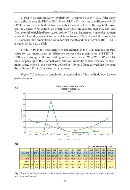
Figure 7.2 shows an example of the application of this methodology for one
particular year.
a)
b)
Fig. 7.2. (a) Example of the results of the model of water balance for a particular year at Junín, Argentina
and (b) numeric results.
90