Chapter 5 Phonons

Chapter 5 

Phonons 

5.1 Introduction 

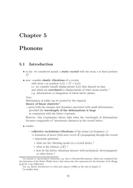
• so far: we considered mainly a static crystal with the atom s at fixed position 

�x 0 

s 

• now: consider elastic vibrations of a crystal, 

with atom s at position �xs(t) = �x 0 

s + �us(t), 

i.e. we consider (small) displacements �us(t) that depend on time 

and which are correlated to displacements of other atoms nearby 1 

e.g. deformations or elongations of whole lattice planes. 

Note: 

Deformation of solids can be treated by the classical 

theory of linear elasticity 2 . 

→ gives both the energies and dynamics associated with small deformations, 

provided the wavelength of the deformations is large 

in comparison with the lattice constants. 

However, this (continuum) theory fails when the wavelength of deformations 

becomes comparable to 3 interatomic distances in the crystal lattice. 

• results: 

– collective excitations/vibrations of the atoms (at frequency ω) 

⇒ formation of waves (with wave vector � K) propagating through the crystal 

→ important questions: 

∗ what are the vibrating modes in a crystal lattice ? 

∗ what is the relation ω( � K) ? 

∗ how do the lattice vibrations interact with mechanical, electromagnetic 

or other forces ? 

1 in contrast to uncorrelated vibrations, e.g. due to thermal fluctuations, which was considered for 

the derivation of the Debye-Waller factor that enters into the expression for the intensity of the Bragg 

peak for x-ray diffraction 

2 see e.g. Kittel Introduction to solid state physics (1966) at the end of chapter 3 

3 or smaller than 

81

82 Chapter 5 Phonons 

– lattice vibrations have particle-like character 

quantum mechanical treatment (particle-wave-dualism): 

propagating waves ↔ phonons with energy �ω (analogy to photons) 

– importance of phonons: 

∗ determine many thermodynamic properties of a crystal 

(e.g. specific heat) 

∗ contribution to thermal conductivity 

∗ interaction with electrons 

→ large contribution to resistivity in metals 

→ formation of (”Cooper pairs”) in (’conventional’) superconductors 

∗ absorption/emission of light in semiconductors 

∗ ... 

• How many modes of oscillations can exist in a crystal with N atoms? 

– 1 atom: 3 degrees of freedom (translation in x, y, z direction 4 ) 

– 2 uncoupled atoms: 2×3 degrees of freedom 

– 2 coupled atoms: also 6 degrees of freedom: 

3 × translation 

2 × rotation (perpendicular to the line connecting the 

atoms) 

1 × oscillation 

– N uncoupled atoms: 3N degrees of freedom (translation) 

– N coupled atoms: also have to have 3N degrees of freedom: 

3 × translation (crystal as a whole) 

3 × rotation (crystal as a whole) 

⇒ 3N − 6 × oscillation 

One finds: the 3N −6 degrees of freedom for oscillations can be classified 

into relatively simple modes of oscillations characterized 

by their dependence ω( � K) (’dispersion relation’) 

4 neglecting rotational motion of the single atoms

5.1 Introduction 83 

Most simple situation is obtained in the [100], [110] and [111] propagation directions 

of cubic crystals (correspond to directions along the cube edge, the face diagonal and 

the body diagonal, respectively). 

If a wave is propagating along one of these directions entire planes of atoms move in 

phase with displacements either parallel (’longitudinal) or perpendicular (’transverse’) 

to the direction of the wavevector � K 

⇒ allows simple description of the displacement of a whole plane s from its equilibrium 

position 

⇒ 1-dimensional problem 

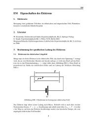
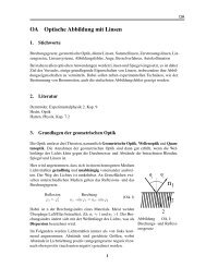
Each wavevector has three ’polarization’ modes – one longitudinal (Fig.5.1) and two 

transverse (Fig.5.2). 

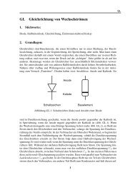
Figure 5.1: (Dashed lines) Planes of atoms when in equilibrium. (Solid lines) Planes 

of atoms when displaced as for a longitudinal wave. The coordinate u measures the 

displacement of the planes [from Kittel, Introduction to solid state physics (1996); 

Fig.4.2]. 

Figure 5.2: Planes of atoms as displaced during passage of a transverse wave [from 

Kittel, Introduction to solid state physics (1999); Fig.4.3].


5.2 1-dimensional chain of identical atoms 

Chain consists of N atoms with masses M. 

• allow only motion of atoms along x-direction 

→ one degree of freedom corresponds to translation of the whole chain along x 

⇒ N − 1 degrees of freedom for oscillations 

• arrangement of atoms: 

Figure 5.3: Displacement of atoms in 1dimensional 

chain 

Atoms located at positions xs = sa + us(t) with lattice constant a 

• choose for simplicity periodic boundary conditions: 

Atom 1 has always same position and momentum as atom N + 1 

(in open chain: e.g. atom 1 and atom N is fixed in space) 

Force acting on atom s due to atom s + 1: 

Fs = C(us+1 − us) , with force constant C (5.1) 

Fs is linear in the displacements → Hooke’s law – is valid if deflection us is not 

too large 

For simplicity we consider only interactions with nearest neighbors s + 1 and s − 1; 

then the total force acting on atom s is 

Fs = C(us+1 − us) + C(us−1 − us) (5.2) 

⇒ equations of motion of atoms (s = 1 . . . N) with mass M: 

M d2 us 

dt 2 ≡ Müs = C(us+1 + us−1 − 2us) (5.3) 

Ansatz for time dependence of displacements: us = u (0) 

s e −iωt 

⇒ üs = −ω 2 us in (5.3) 

⇒ −Mω 2 u 0 s = C(u 0 s+1 + u 0 s−1 − 2u 0 s) (5.4) 

which is a difference equation in the displacements u, 

with travelling wave solutions 

u 0 s = ue iKsa 

(= longitudinal wave along x with wavevector K) 

(5.5) 

with (5.5) in (5.4) ⇒ −Mω 2 ue iksa = Cu(e iK(s+1)a + e iK(s−1)a − 2e iKsa ) (5.6) 

(divide by u · e iKsa )

5.2 1-dimensional chain of identical atoms 85 

⇒ Mω 2 = −C(e iKa + e −iKa − 2) = 2C(1 − cos Ka) (5.7) 

This finally yields the dispersion relation ω(K) 

ω 2 = 2C 

� 

4C 

(1 − cos Ka); ω = 

M M 

for the travelling wave us = ue i(sKa−ωt) . 

(with 2 cos x = e i x + e −ix ) 

� � 

� 

� 

Ka � 

�sin � 

2 � 

(5.8) 

(with √ 1 − cos x = | sin(x/2)|) 

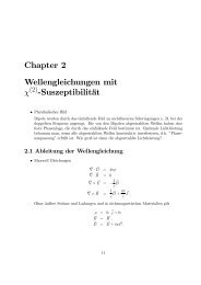
Figure 5.4: Dispersion relation 

ω(K) of monatomic linear chain. 

• The regime of physically significant values of K is limited due to e iKa ≡ e i(Ka+2πn) , 

(with n = 0, ±1, ±2, . . .) 

→ independent K vectors are only specified within the interval 

−π ≤ Ka ≤ π ⇔ − π 

a 

≤ K ≤ π 

a 

1. Brillouin zone 

• connection between K values within and outside the 1. Brillouin zone: 

A vector K outside the 1. Brillouin zone can be transformed into a vector K ′ 

inside the 1. Brillouin zone by subtracting or adding a multiple of 2π/a, 

i.e. via the transformation K ′ = K + G where G is a reciprocal lattice vector. 

The displacement ration of neighboring atoms is 

us+1 

us 

= u e[i(s+1)Ka] 

u e isKa 

= eiKa 

hence 

us+1 

= e 

us 

iKa = e i2πn 

�� · e 

=1 

i(Ka−2πn) ≡ e iK′ a 

i.e. any displacement can always be described by a wavevector within the 

1. Brillouin zone. 

(5.9) 

(5.10)


In other words: 

The range of −π ≤ Ka ≤ π covers all independent values of the exponential 

e iKa = us+1/us. I.e., saying that two adjacent atoms are out of phase by 0.3π or 

2.3π has the same physical meaning, as shown in the figure below. 

Figure 5.5: The wave represented by the solid curve conveys no information not given 

by the dashed curve. Only wavelengths longer than 2a are needed to represent the 

motion [from Kittel, Introduction to solid state physics (1996); Fig.4.5]. 

• limit of long wavelength: 

if K ≪ a ⇔ wavelength λ ≡ 2π/K ≫ a 

one can approximate in (5.8) |sin(x)| ≈ x, i.e. 

� 

C 

ω ≈ Ka ∝ K (5.11) 

M 

this limit corresponds to the continuum approximation 

• there exists a maximum value for the frequency ωmax = (4C/M) 1/2 , 

reached when the K ’vector’ lies on the boundary of the 1. Brillouin zone 

→ Kmax = ±π/a ⇔ λmin = 2a. 

Typical values in solids are ωmax ∼ 10 13 Hz. 

Solution at Kmax = ± π 

a (i.e. at the zone boundary): Kmaxsa = ±sπ, hence 

us = u · e ±iπs e −iωt = u · (−1) s e −iωt 

= standing wave (due to Bragg reflection at the zone boundary) 

compare with Bragg condition 2d sin θ = n · λ: 

d = a, 

θ = π/2 ⇒ sin θ = 1 ⇒ 2d sin θ = 2a 

n = 1 

λ = 2π/Kmax = 2π/(π/a) = 2a ⇒ n · λ = 2a q.e.d

5.2 1-dimensional chain of identical atoms 87 

• group velocity: 

The group velocity of a wave packet is given as the slope of the dispersion curve 

ω(K) 

vg = dω 

or �vg = gradKω( 

dK 

� K) (5.12) 

(corresponds to the velocity of energy propagation in a crystal) 

With the dispersion relation (5.8) the group velocity is 

� 

Ca2 Ka 

vg = cos 

M 2 

limit of long wavelength: 

vg = 

� C 

M 

· a = const. 

corresponds to sound waves with long wavelength; 

(5.13) 

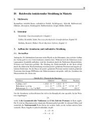
Figure 5.6: Group velocity vs. K, for 

monatomic 1-dim. chain. vg = 0 at the 

zone boundary, i.e. there is no transport 

of energy 

• Distribution of the N − 1 oscillatory degrees of freedom 

from periodic boundary conditions us = us+N 

⇒ e iKsa = e i[K(s+N)a+2πn] 

⇒ NKa = 2πn 

⇒ K = 2π 

n, n = −N/2 ≤ n ≤ N/2) 

Na 

⇒ N discrete values for K; with K = 0 corresponding to translation 

⇒ oscillatory degrees of freedom are being ”used up” 

just within the 1. Brillouin zone.


• generalization to 3D: 

we used Hooke’s law F = C · u which is valid in that form only in one dimension; 

in 3D this relation becomes more complex: 

– replace force by stress 5 field (’Spannungsfeld’) ↔ σ(tensor; 3×3 matrix) 

– replace displacement by strain field (’Dehnungsfeld’) ↔ ε (tensor; 3×3 matrix) 

– then: ↔ σ= ↔ 

C ↔ e ; 

↔ 

C is a tensor (4. Stufe) with 81 componentsCiklm; 

hereby: 21 components are independent of each other 

(s. Kittel, chapter 3) 

• derivation of force constants from experiment 

So far, we used the approximation of only nearest neighbor interactions, i.e. for 

the force on atom s from the displacement of atom s + p we only considered 

p = ±1. 

Particularly in metals the effective forces can be of quite long range, i.e. interactions 

of lattice planes up to 20 lattice spacings apart from each other (i.e. p = 20) 

can be significant. 

For that case one can find a generalization of the dispersion relation (5.7) to p 

nearest neighbors as 

ω 2 = 2 � 

Cp(1 − cos pKa) 

M 

(5.14) 

Solving for the interplanar force constants Cp at range pa yields 

Cp = − Ma 

2π 

p>0 

for a structure with a monatomic basis. 

� +π/a 

dK ω 

−π/a 

2 K cos pKa (5.15) 

The measurement of the dispersion relation hence allows the determination of 

the range of the interplanar forces. 

5 stress is defined as force per unit area

5.3 1-dimensional chain of two different atoms 89 

5.3 1-dimensional chain of two different atoms 

Atoms shall have masses M1, M2 

Atoms with masses M1 are displaced by us−1, us, us+1,. . . 

and atoms with masses M2 by vs−1, vs, vs+1,. . . 

Figure 5.7: 1-dimensional chain of two 

different atoms with displacements vs, . . . 

and us, . . . 

The force constant shall be again denoted as C, i.e. force between two (different) 

neighboring atoms is F = C(vs − us) (Hook’s law). 

⇒ equations of motion: 

M1üs = C · (vs + vs−1 − 2us) 

Ansatz: 

travelling waves, now with different amplitudes 

M2¨vs = C · (us+1 + us − 2vs) (5.16) 

us = u · e i(sKa−ωt) 

vs = v · e i(sKa−ωt) 

(5.17) 

where the lattice constant a is defined as the distance between nearest neighbors of 

atoms with same mass (for zero displacement). 

Substitution of (5.17) in (5.16) yields 

−ω 2 M1u = Cv[1 + e −iKa ] − 2Cu 

−ω 2 M2v = Cu[1 + e iKa ] − 2Cv (5.18) 

This system of linear equations has a solution only if the determinant of the coefficients 

of the unknowns u, v vanishes 

� 

� 

� 

� 

det � 

� 

� 

� = 0 (5.19) 

hence 

2C − M1ω 2 −C · [1 + e −iKa ] 

−C · [1 + e iKa ] 2C − M2ω 2 

M1M2ω 4 − 2C(M1 + M2)ω 2 + 2C 2 (1 − cos Ka) = 0 (5.20)


• solution for ka ≪ 1 : 

with cos Ka ≈ 1 − 1 

2 K2 a 2 + . . . one finds the two solutions 

and 

ω 2 � 

1 

≈ 2C 

ω 2 ≈ 

M1 

+ 1 

� 

M2 

C 

2(M1 + M2) K2 a 2 

• solution at the zone boundary Kmax = ± π 

a : 

cos Ka = −1, hence 

ω 2 = 2C 

M1 

”optical branch” (5.21) 

”acoustical branch” (5.22) 

and ω 2 = 2C 

M2 

(5.23) 

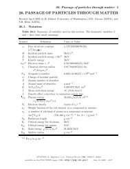
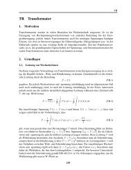
The full dispersion relatione, including the discussed limiting cases is shown below for 

the case M1 > M2. 

Figure 5.8: Optical and acoustical branches of the dispersion relation for a diatomic 

linear lattice, showing the limiting frequencies at K = 0 and K = Kmax = π. 

The a 

lattice constant is a [from Kittel, Introduction to solid state physics (1996); Fig.4.7].

5.3 1-dimensional chain of two different atoms 91 

The figure below shows the atom displacements transverse to the K vector. 

Figure 5.9: Transverse optical 

and transverse acoustical waves 

in a diatomic linear lattice, illustrated 

by the particle displacements 

for the two modes at the 

same wavelength. [from Kittel, 

Introduction to solid state 

physics (1996); Fig.4.10]. 

• For the transverse optical (TO) branch at K = 0 one finds on substitution of 

(5.21) in (5.18) 

u 

v 

= −M2 

M1 

The minus sign means that the atoms vibrate against each other. 

(5.24) 

If the two atoms have opposite charges one can excite this type of vibration by 

the electric field of an incident light wave ⇒ ’optical’ mode. 

• In the K = 0 limit of (5.21) one finds as a solution for the transverse acoustical 

branch v = u. 

This means that the atoms move together, as in long wavelength acoustical vibrations 

⇒ ’acoustical’ mode. 

• frequency gap: 

For certain frequencies – here for (2C/M1) 1/2 < ω < (2C/M2) 1/2 – there are no 

wavelike solutions. 

→ characteristic for polyatomic lattices 

Solutions for real ω yield a complex wavevector 

⇒ us = u · e −s|K|a · e −iωt → damping in space! 

Note: the 2N degrees of freedom ”fit” again into the 1. Brillouin zone.


5.4 Generalization and examples 

• extension to p atoms in the basis: p branches in 1D 

• extension to 3D: 

– one longitudinal (”L”) and two transverse (”T”) ’polarization’ modes 

E.g. for NaCl or diamond with p = 2 atoms in the primitive cell: 

for each of the three polarization modes (1L and 2T) one gets two branches 

(acoustical and optical) 

⇒ 2 × 3 = 6 branches 

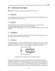
The figures below show examples for germanium and KBr also with p = 2 

atoms per primitive cell. 

– p atoms in primitive cell ⇒ 3p branches: 

3 acoustical branches (1LA, 2TA) 

3p − 3 optical branches → (p − 1)LO, 2(p − 1)TO 

(valid for each direction � K) 

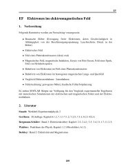
Figure 5.10: Phonon dispersion relations in the [111] direction: Left in germanium 

at 80 K. The two TA phonon branches are horizontal at the zone boundary position 

Kmax = 2π 

a · � � 

1 1 1 . The LO and TO branches coincide at K = 0 ; this also is a conse- 

2 2 2 

quence of the crystal symmetry of Ge. The results were obtained with neutron inelastic 

scattering by G. Nielsson and G. Nelin. Right in KBr at 90 K, after A.D.B. Woods 

et al. The extrapolation to K = 0 of the TO and LO branches are called ωT and ωL. 

[from Kittel, Introduction to solid state physics (1996); Fig.4.8].

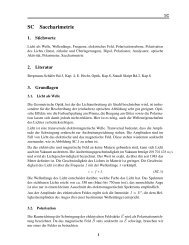
5.4 Generalization and examples 93 

Example: Silicon 

Si crystallizes in the diamond lattice with p = 2 atoms per cell. The figure below shows 

the Brillouin zone of such a cubic crystal. 

Figure 5.11: Brillouin zone of cubic crystals. 

Some points and lines of high symmetry 

are drawn. Γ denotes the center 

(0, 0, 0), the point X is given by 2π(0, 

1, 0), 

a 

the point L by π(1, 

1, 1) and the point 

a 

K by 3π(0, 

1, 1) [from Bergmann-Schaefer, 

2a 

Lehrbuch der Experimentalphysik, Bd. 6 

Festkörperphysik (1992); Abb.1.18]. 

Due to p = 2, silicon has 6 phonon branches which are degenerate along the lines ∆ 

and Λ. 

Figure 5.12: Dispersion of phonons in Si. Shown is the phonon energy �ω, with phonon 

frequency ω. Γ, X, K and L denote different points and ∆, Σ and Λ different lines in 

the Brillouin zone, as defined in fig. 5.4. Extending the line ¯ ΓK outside the Brillouin 

zone one reaches a point which is equivalent to X. L and T means longitudinally 

and transversely polarized wave, respectively, A, acoustical wave, and O optical wave. 

[from Bergmann-Schaefer, Lehrbuch der Experimentalphysik, Bd. 6 Festkörperphysik 

(1992); Abb.1.19].


Example: Tl2Ba2CaCu2O8 (high-Tc superconductor) 

The figures below show the Brillouin zones of a body-centered tetragonal (bct) and a 

simple tetragonal (st) lattice of a complex cuprate superconductor, together with the 

calculated phonon dispersion relations of the bct structure. 

Figure 5.13: Left: Brillouin zones of the body-centered tetragonal (top) and simple 

tetragonal (bottom) lattices. The symmetry directions along which the dispersion 

curves are displayed are indicated with heavy lines. For the body-centered tetragonal 

lattice, X = (1, 1, 0) π 

a , G1 

� 

= (1, 0, 0) 1 + a2 

c2 � 

π 

π 

π 

, and Z = (0, 0, 2) = (2, 0, 0) . For 

a c a 

the simple tetragonale lattice, X = (1, 0, 0) π 

π 

π 

, M = (1, 1, 0) and Z = (0, 0, 1) . a, a, c 

a a c 

are the sides of the conventional unit cells of both lattices. Right: Phonon dispersion 

curves of bct Tl2CaBa2Cu2O3 (2:1:2:2:8) along symmetry directions of the bct Brillouin 

zone. [from Kulkarni et al., Physical Review B 43, 5451 (1991); Fig. 1 and 3].

5.5 Quantized lattice vibrations: Phonons 95 

5.5 Quantized lattice vibrations: Phonons 

Quantum mechanics: Energy of a wave with frequency ω: 

� 

E = n + 1 

� 

�ω 

2 

with n: number of quantum ’particles’; n = 0, 1, 2, . . . 

electromagnetic (light) wave: ”Quantum particle” = Photon 

lattice vibrations: ”Quantum particle” = Phonon 

here: 

E = (n+ 1)�ω 

is the energy of an elastic mode of frequency ω when the mode is excited 

2 

to the quantum number n, 

i.e. the mode is occupied by n phonons. 

For n = 0 → E = �ω/2 = zero point energy of the mode. 

Occurs for both – phonon and photon – due to their equivalence to a quantum mechanical 

harmonic oscillator of frequency ω 

Phonon momentum: 

A phonon of wavevector � K can interact with particles as if it had a momentum �p = � � K 

However, a phonon does not carry a physical momentum 

(except for � K = 0, corresponding to the translation of a crystal as a whole) 

Note: � K is only defined modulo a reciprocal lattice vector � G. 

Explanation (in the ’particle picture’): 

the crystal as a whole can change its momentum by � � G during Bragg 

reflection (recoil); 

Recoil energy E recoil = (� � K) 2 /2M crystal very small, since M crystal very large 

• possible interactions of phonons with: 

– electrons, neutron, photons,. . . 

– other phonons (due to anharmonic terms in the elastic energy) 

selection rules in a crystal: 

govern allowed transitions between quantum states, 

e.g. for elastic scattering of an x-ray photon by a crystal we found 

� k ′ = � k + � G (5.25) 

where � G is a reciprocal lattice vector, � k is the wavevector of the incident photon 

and � k ′ is the wavevector of the scattered photon.


inelastic scattering by phonons: 

scattering of a photon with a phonon involved can be described by either 

� k ′ + � K = � k + � G (5.26) 

i.e. the creation (emission) of a phonon of wavevector � K or by 

� k ′ = � k + � K + � G (5.27) 

i.e. the absorption of a phonon � K during the scattering process. 

• interaction with neutrons: 

Inelastic scattering of neutrons by absorption or emission of a phonon is a widely 

used method for the determination of the phonon dispersion relation ω( � K) 

Kinematics are described by 

→ conservation of momentum: 

� kneutron + � G = � k ′ neutron ± � Kph 

(5.28) 

(”±”: creation/anihilation of a phonon) 

Here, � G is chosen such that � K lies in the 1. Brillouin zone. 

→ conservation of energy: 

� 2 k 2 neutron 

2mn 

= �2k ′2 

neutron 

± �ωph 

2mn 

(5.29) 

(”±”: creation/anihilation of a phonon) 

Experimental determination of ω( � K) is based on the two conservation laws (5.28), 

(5.29). 

Then in the experiment, one needs to find the energy gain or energy loss of the 

scattered neutrons as a function of the scattering direction � k − � k ′ . 

Advantage of using neutrons: 

→ Eneutron, λneutron are comparable to Eph, λph

5.5 Quantized lattice vibrations: Phonons 97 

Figure 5.14: Phonon dispersion in GaAs as obtained from neutron scattering (after 

Strauch and Dorner). The different points and lines on/along the wave vector axis 

are defined in Fig.5.11; ν is the frequency [from Bergmann-Schaefer, Lehrbuch der 

Experimentalphysik, Bd. 6 Festkörperphysik (1992); Abb.1.30].


5.6 Thermal properties of phonons 

5.6.1 contribution to the heat capacity 

Heat capacity is very sensitive to elementary excitations and ordering phenomena in 

crystals (electrons, phonons, magnetic order, spin waves, superconductivity etc.). 

Each phenomenon has very specific properties (e.g. T dependence) 

⇒ heat capacity is a well suited probe; 

particular advantage: detects volume properties 

In general one defines the heat capacity either as 

CV ≡ (∂U/∂T )V at constant volume or 

Cp ≡ (∂U/∂T )p at constant pressure; 

here T is the temperature and U is the energy. 

The phonon contribution to the heat capacity of a crystal is called the 

lattice heat capacity Clat. 

some results from quantum statistics (without proof): 

A system of quantum particles (e.g. vibrations) shall be characterized by energies En 

(n: index number) 

– question: What is the probability f(En) of finding a quantum particle 

at the energy En? 

– answer: depends on the nature of the particle and on temperature: 

– particles with semi-integer spin (e.g. 1�) 

= fermions, 

2 

e.g. electrons: 

1 

f(En) = 

e (En−µ)/kBT Fermi-Dirac distribution function 

+ 1 

(5.30) 

Here, µ is the(chemical potential), which has to be determined in such 

a way that the number of particles in the system (e.g. all electrons in the 

crystal) is conserved. 

– particles with integer spin (e.g. 0�, 1�) = bosons, 

e.g. photons, phonons: 

f(En) = 

1 

e (En−µ)/kBT − 1 

Bose-Einstein distribution function 

particular property of photons, phonons: 

there is no conservation of the number of particles ⇒ µ = 0 

classical statistics (for distinguishable particles) yields probability 

f ∝ e −(E−µ)/kBT 

(5.31) 

Boltzmann distribution function (5.32)

5.6 Thermal properties of phonons 99 

Back to the phonon heat capacity: 

• internal energy of a vibrating crystal: 

U = � � 1 

e�ω( � �ω( 

K)/kBT − 1 � K) (5.33) 

p 

� k 

= energy �ω( � K) multiplied by the probability to have a state occupied at this 

energy – and with summation over all wave vectors � K and polarization states p. 

• there do exist a lot of states � K 

⇒ � � K can be transformed into an integral � dω · D(ω), 

with D(ω): number of states within the frequency interval dω 

(= ”density of states or ”Zustandsdichte”) 

• determination of D(ω): 

– consider cube with length L, plus periodic boundary conditions 

→ possible vibrating states 

(compare to linear chain with L = Na where we found K = 2πn/Na): 

Kx = 0, ±2π/L, ±4π/L, . . . ; Ky, Kz analog 

→ 1 state per 

� �3 2π 

= 

L 

8π3 

V 

→ number of states in � K space within a sphere with radius K: 

NK = 4π 

3 K3 · V 

8π 3 

(for each polarization p) 

The density of states for each polarization type is hence given by 

D(ω) = dNK 

dω 

• next task: determine dK/dω 

= dNK 

dK 

· dK 

dω 

V K2 dK 

= · 

2π2 dω 

(5.34) 

(5.35) 

(5.36)


→ Debye model of density of states: 

Assumption: 

The velocity of sound is taken as constant for each polarization type 

(like in classical elastic continuum). 

Gives simple dispersion relation 

with sound velocity vs. 

Hence, the density of states is given as 

ω = vsK (5.37) 

D(ω) = 

V ω2 

2π2v3 s 

Remark: 

Debye model is o.k. for acoustical phonons; 

at sufficiently low temperature 6 mainly those phonons are excited 

(energy of the optical phonons is large for all � K!) 

With N primitive cells in the crystal volume V : 

The total number of acoustic phonon modes is N 

(5.38) 

From (5.35) we know then that all N vibrating states are located within the volume 

(in K space) 

N = V 

8π3 4π 

3 K3 = V 

8π3 4π 3 

(ω/vs) (5.39) 

3 

This relation defines a maximum frequency, or ’cutoff’ frequency 

� 2 3 6π v 

ω ≡ ωD = 

sN 

V 

� 1 

3 

(”Debye frequency”) (5.40) 

With the dispersion relation one gets the corresponding cutoff wavevector 

KD = ωD 

vs 

� 2 6π N 

= 

V 

� 1 

3 

(”Debye wave vector”) (5.41) 

Note: ωD and KD depend only on the density N/V , which is physically reasonable. 

6 compare distribution function


Thermal energy for each polarization type: 

Now we can use the obtained density of state to make the transformation from the 

summation over all K vectors in (5.33) to the integration over all possible frequencies 

up to the maximum frequency ωD 

� 

U = 

�ω 

dωD(ω) 

e�ω/kBT = 

− 1 

If vs is identical for all three polarizations 

⇒ U = 3 · 

with x ≡ �ω 

kBT and 

V � 

2π 2 v 3 s 

� ωD 

0 

dω · 

ω 3 

� ωD 

0 

dω · 

e �ω/kBT − 1 = 3V k4 B 

xD ≡ �ωD 

kBT 

≡ Θ 

T 

V ω2 

2π2v3 s 

4 T 

2π2v3 s�3 · 

� xD 

Here we defined Θ = �ωD/kB as the ”Debye temperature” 

Θ = �vs 

kB 

� 6π 2 N 

V 

� 1 

3 

With this definition we can express the thermal energy as 

U = 9NkBT 

� �3 � xD T 

dx 

Θ 0 

x3 

ex − 1 

0 

�ω 

e �ω/kBT − 1 

dx x3 

e x − 1 

with N atoms in the specimen. Thus, the heat capacity (plotted in Fig.5.15)) is 

Cv = ∂U 

∂T 

= 9NkB 

� �3 � xD T 

dx 

Θ 0 

x4ex (ex − 1) 2 

(5.42) 

(5.43) 

(5.44) 

(5.45) 

(5.46) 

(5.47) 

Figure 5.15: Heat capacity CV of a solid, according to the Debye approximation. [from 

Kittel, Introduction to solid state physics (1996); Fig.5.7].


For low temperature: xD → ∞ 

(Debye approximation is anyway only a good approximation at low temperature) 

Then: � xD 

0 

dx x3 

e x − 1 → 

� ∞ 

0 

dx x3 

e x − 1 

U = 3π4NkBT 4 

5Θ3 and cv = 12π4NkBT 3 

5Θ3 cV ∝ T 3 

= π4 

15 

≈ 234NkB 

� �3 T 

Θ 

(5.48) 

(5.49) 

(Debye’s T 3 law) (5.50) 

’simple’ explanation: 

We have 3N possible modes (N: number of primitive cells). 

Only those modes having �ω < kBT will be excited at low temperature to an energy 

close to kBT . 

Hence, from the available volume in � K space only a fraction (ωT /ωD) 3 = (T/Θ) 3 will 

be occupied by excited modes. 

�3; ⇒ number of excited phonons ≈ 3N � T 

Θ 

each phonon has energy kBT 

⇒ energy ∼ 3NkBT (T/Θ) 3 , and CV ∼ 12NkB(T/Θ) 3 

The range of validity of the T 3 is below 0.1Θ. 

For T ≫ Θ the heat capacity approaches the classical value 3NkB. 

Typical values for Θ: 

Li : 334 K 

C : 2230 K 

Au : 165 K 

K : 91 K 

Figure 5.16: Heat capacity of silicon and germanium. Not the decrease at low temperatures. 

To convert a value in cal/mol·K to J/Mol·K, multiply by 4.186. [from Kittel, 

Introduction to solid state physics (1996); Fig.5.8].


Einstein model of the density of states: 

consider N oscillators at the same frequency ω0 

(o.k. for many optical phonons) 

Density of states: 

Thermal energy: 

heat capacity: 

�ω0 

U = 3N 

e�ω0/kBT − 1 

as plotted in the figure below 

Cv = 3NkB 

D(ω) = Nδ(ω − ω0) (5.51) 

� �2 �ω0 

kBT 

”3” due to polarization (5.52) 

e �ω0/kBT 

(e �ω0/kBT − 1) 2 

(5.53) 

Figure 5.17: Comparison of experimental values of the heat capacity of diamond with 

values calculated on the earliest quantum (Einstein) model, using the characteristic 

temperature ΘE = �ω/kB = 1320 K. To convert to J/Mol·K, multiply by 4.186. [from 

Kittel, Introduction to solid state physics (1996); Fig.5.11]. 

For low temperature: Cv ∝ e −�ω0/kBT 

(not as good as Debye model which is in better agreement with experimental data) 

For high temperature: Cv → 3NkB 

(reproducing the ”Dulong-Petit value”, as the Debye model does)


General expression for the density of states: 

A general expression for D(ω) – the number of states per unit frequency range – requires 

the knowledge of the phonon dispersion relation ω( � K). 

The number of allowed K values for which the phonon frequency is between ω and 

ω + dω is 

D(ω)dω = V 

8π3 � 

d 3 K (5.54) 

(We found earlier that we have one state per V/(8π 3 ); 

The integral goes over the volume of the shell in � K space bounded by the two surfaces 

on which the phonon frequency is constant and either ω or ω + dω) 

Problem: 

evaluate the volume of this shell ! 

We consider a surface of constant ω in � K space as shown in the figure below. 

Here, we denote dSω an element area on this surface 

shell 

Figure 5.18: Element of area dSω on a 

constant frequency surface in K space. 

The volume between two surfaces of constant 

frequency at ω and ω + dω is 

equal to � dSωdω/|∇Kω| [from Kittel, Introduction 

to solid state physics (1996); 

Fig.5.12]. 

With the perpendicular distance dK⊥ between the surfaces of constant ω and constant 

ω + dω (see next figure) one gets: 

� 

d 3 � 

k = dSωdk⊥ 

(5.55) 

shell


Figure 5.19: The quantity dK⊥ is the perpendicular 

distance between two constant frequency surfaces in 

K space, one at frequency ω, the other at frequency 

ω + dω [from Kittel, Introduction to solid state physics 

(1996); Fig.5.13]. 

furthermore | � ∇ � K ω|dK⊥ = dω; here � ∇ � K is the gradient in K space 

Note: 

dω 

⇒ dSωdK⊥ = dSω 

| � ∇K� ω| 

⇒ D(ω) = V 

8π3 � 

dSω 

vg 

ω=const. 

• Integral goes over area of constant ω in � K space 

dω 

= dSω 

vg 

• D(ω) can contain singularity points = ”Van-Hove singularities”, 

if the group velocity vg = 0 

(this is e.g. the case at Brillouin zone boundary) 

Figure 5.20: Density of states as a function of frequency for (a) a solid according to 

the Debye model and (b) an actual crystal structure. The spectrum for the crystal 

starts as ω 2 for small ω, but discontinuities develop at singular points [from Kittel, 



5.6.2 Thermal expansion of solids 

So far, we only considered a linear force-displacement relation to describe lattice vibrations 

(Hook’s law). 

This leads to a potential energy which is quadratic in the interatomic displacements 

(harmonic theory). 

As one of its consequences there should be no thermal expansion which we will consider 

now: 

Naive view: solid expands, while atoms oscillate 

about their equilibrium position. 

but: if one considers only harmonic oscillations, the average position of 

the atom remains unchanged, no matter how large the amplitude 

of oscillation is. 

⇒ thermal expansion of solids results from anharmonic potential 

Quantitatively: 

• Taylor expansion of the potential energy of an atom in the crystal potential 

(equilibrium position shall be at x = 0) 

(consider 1-dim. solid) 

– only 1. term: ”harmonic approximation” 

– additional terms: ”anharmonic” 

U(x) = cx 2 − gx 3 − fx 4 . . . (5.56) 

∗ term −gx 3 : Asymmetry in mutual repulsion of neighboring atoms 

∗ term −fx 4 : Softening of the vibrations (attenuation of the ”spring constant” 

at large amplitudes 

• average displacement of the atom: 

with β = 1 

bility to 1. 

– use Boltzmann distribution which weights all possible values of displacement 

x with the factor e −U(x)/kBT (classical statistics o.k. for high temperatures) 

kBT 

⇒ 〈x〉 = 

� ∞ 

−∞ � ∞ 

−∞ 

dx · x · e −βU(x) 

dx · e −βU(x) 

(5.57) 

. The denominator is a normalization factor; normalizes the total proba


– expand the integrands for small displacements 

i.e. such that the anharmonic terms in the energy are small as compared to kBT 

� 

dx · xe −βU(x) � 

≈ dx · e −βcx2 

(x + βgx 4 + βfx 5 ) = 3√π g 

β−3/2 

4 c5/2 � 

dx · e −βU(x) � 

≈ dxe −βcx2 

� 

π 

= 

βc 

〈x〉 ≈ 3g 

2c 2 kBT (5.58) 

⇒ thermal expansion proportional to T due to 3. order term in the potential 

Measurements of the lattice constant a vs. temperature of solid argon are shown below. 

The slope da/dT is proportional to the thermal expansion coefficient (vanishes at low 

T ), which is significant at high T . 

Figure 5.21: Lattice constant of solid argon as a function of temperature [from Kittel, 



5.6.3 Phonon contribution to thermal conductivity 

consider long slab with temperature gradient dT/dx 

⇒ there is a steady-state flow of heat 

jU = −KU · dT 

dx 

(5.59) 

here KU is the thermal conductivity coefficient (’Wärmeleitzahl’), and jU is the flux of 

thermal energy (or the energy transmitted across unit area per time) 

requires: 

transfer of thermal energy is a diffusive process, subject to random scattering processes 

inside the slab; 

otherwise jU would only be determined by the temperature difference ∆T at the ends 

of the slab. 

⇒ the random nature of the heat transfer is responsible for 

(i) the development of a thermal gradient, and 

(ii) for the appearance of a mean free path ℓ in the expression of the thermal flux. 

Idea for calculation: consider phonons as a gas of particles 

general result of the kinetic gas theory: KU = 1 

3 

Cvℓ with: 

C: heat capacity per volume 

v: mean particle velocity (here: velocity of sound, few km/s) 

ℓ: mean free path (typically a few nm at 300 K; a few 10 nm at 77 K) 

’Derivation’: 

consider flux of particles n〈vx〉 along x direction (n: density of particles) 

The associated thermal flux is then given by 

ju = −n〈vx〉∆U 

this is due to the fact that a particle will give up energy ∆U = c∆T at temperature T : 

(if particle comes from a region with higher temperature T + ∆T ; 

c: heat capacity of the particle) 

between end points of a mean free path ℓ: 

with ℓ = vτ and C = nc 

∆T = dT dT 

ℓ = 

dx dx 〈vx〉τ with τ: mean collision time (5.60) 

⇒ ju = −n〈v 2 x〉cτ dT 

dx 

jU = − 1 

3 Cvl 

dT 

� �� dx 

=KU 

= −1 

3 n〈v2 〉cτ dT 

dx 

(5.61) 

(q.e.d.) (5.62)


Discussion of heat transport mediated by phonon gas 

Above, we introduced the mean free path for phonon scattering to derive the heat 

transport mediated by phonons. 

→ required: inelastic scattering processes, which restore thermal equilibrium. 

→ collisions of phonons with lattice defects, or with surface: 

does not work, because elastic – the phonon frequency remains unchanged 

→ collisions between phonons: 

(note: in this case anharmonic terms in the potential energy U(x) of the 

atoms are important!) 

in general: � K1 + � K2 = � K3 + � G 

for � G = 0: Normal processes (N processes) 

for � G �= 0: Umklapp-Processes (U processes) 

N processes: 

The total phonon momentum is � J = � � J n � K � � K; 

here n � K is the number of phonons with wavevector � K. 

The change in total phonon momentum is 

∆ � J = � J ′ − � J = � � K3 − � � K1 − � � K2 = �( � K3 − � K1 − � K2) = 0 (5.63) 

i.e. for N processes the total phonon momentum is conserved 

A distribution of hot phonons with � J �= 0 propagating down a rod will leave � J 

unchanged, i.e. N processes will not be able to establish thermal equilibrium. 

⇒ no thermal resistance, as illustrated in Fig.5.23(top) for the flow of hot gas 

molecules in a tube with frictionless walls and in Fig.5.24(top). 

U processes: 

⇒ U processes are responsible for the thermal conductivity due to phonons 

as they allow change of the total phonon momentum (Fig.5.23(bottom), 

5.24(bottom)) 

Figure 5.22: (a) Normal (N) 

and (b) Umklapp (U) phonon 

collision processes in the reciprocal 

lattice of a 2-dim. square 

lattice. The square represents 

the 1. Brillouin zone [from Kittel, 

Introduction to solid state 

physics (1999); Fig.5.17c].


Figure 5.23: (top) Flow of gas molecules in a state of drifting equilibrium down a long 

open tube with frictionless walls. Elastic collision processes among the gas molecules do 

not change the momentum or energy flux of the gas because in each collision the velocity 

of the center of mass of the colliding particles and their energy remain unchanged. 

Thus energy is transported from left to right without being driven by a temperature 

gradient. Therefore the thermal resistivity is zero and the thermal conductivity is 

infinite. (bottom) The usual definition of thermal conductivity in a gas refers to 

a situation where no mass flow is permitted. Here the tube is closed at both ends, 

preventing the escape or entrance of molecules. With a temperature gradient the 

colliding pairs with above-average center of mass velocities will tend to be directed to 

the right, those with below-average velocities will tend to be directed to the left. A 

slight concentration gradient, high on the right, will be set up to enable the net mass 

transport to be zero while allowing a net energy transport from the hot to the cold 

end. [from Kittel, Introduction to solid state physics (1999); Fig.5.16a].


Figure 5.24: top: In a crystal we may arrange to create phonons chiefly at one end, 

as by illuminating the left end with a lamp. From that end there will be a net flux 

of phonons toward the right end of the crystal. If only N processes (K1 + K2 = K3) 

occur, the phonon flux is unchanged in momentum on collision and some phonon flux 

will persist down the length of the crystal. On arrival of phonons at the right end we 

can arrange in principle to convert most of their energy to radiation, thereby creating a 

sink for the phonons. Just as in Fig.5.23(top) the thermal resistivity is zero. bottom: 

In U processes there is a large net change in phonon momentum in each collision event. 

An initial net phonon flux will rapidly decay as we move to the right. The ends may act 

as sources and sinks. Net energy transport under a temperature gradient occurs as in 

Fig.5.23(bottom) [after Kittel, Introduction to solid state physics (1999); Fig.5.16cd]. 

→ very high temperatures T > Θ: 

– all phonon modes are excited and the phonon density n ∝ T (compare with 

Bose-Einstein statistics) 

U processes will provide relaxation to thermal equilibrium 

– mean free path ℓ ∝ 1/n ∝ 1/T ⇒ KU ∝ 1/T 

→ low temperatures: 

– number of phonons which are suited to U processes decreases ∝ e −Θ/T 

– ⇒ K ∝ e Θ/T 

→ very low temperatures: 

– mean free paths reaches dimension of the crystal D 

⇒ KU → 1 

3 CvD ∝ T 3 , since C ∝ T 3


example (NaF): 

Figure 5.25: Thermal conductivity of a highly purified crystal of sodium fluoride (NaF), 

after H.E. Jackson, C.T. Walker and T.F. McNelly [from Kittel, Introduction to solid 

state physics (1999); Fig.5.18]. 

Final remarks: 

• in metals: 

additional (strong) heat transport due to electrons 

• some insulators (e.g. sapphire, Al2O3): 

have nevertheless a thermal conductivity which is comparable to metals, 

e.g. maximum ∼200 W/(cmK) at 30 K for sapphire 

• for comparison: 

maximum thermal conductivity of copper is 100 W/(cmK)

Chapter 5 Phonons

You also want an ePaper? Increase the reach of your titles

Delete template?

Save as template?