Thematic Accuracy Assessment Procedures. Version 2 - USGS
Thematic Accuracy Assessment Procedures. Version 2 - USGS
Thematic Accuracy Assessment Procedures. Version 2 - USGS

You also want an ePaper? Increase the reach of your titles
YUMPU automatically turns print PDFs into web optimized ePapers that Google loves.
National Park Service<br />
U.S. Department of the Interior<br />
Natural Resource Program Center<br />
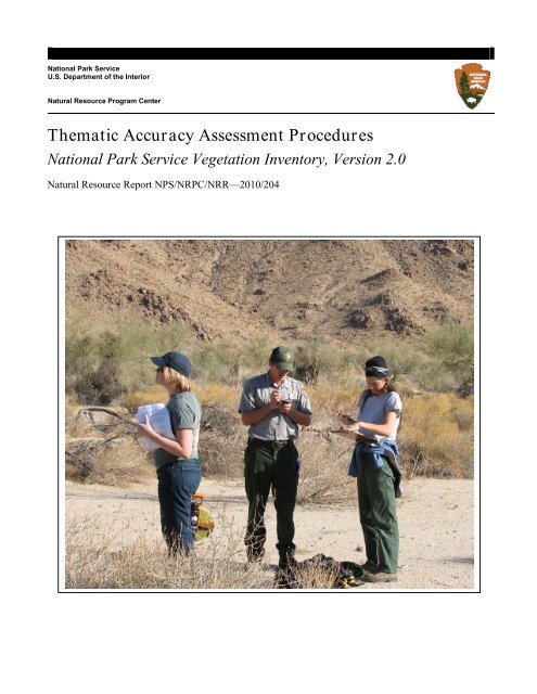
<strong>Thematic</strong> <strong>Accuracy</strong> <strong>Assessment</strong> <strong>Procedures</strong><br />
National Park Service Vegetation Inventory, <strong>Version</strong> 2.0<br />
Natural Resource Report NPS/NRPC/NRR—2010/204
ON THE COVER<br />
National Park Service staff record field data for a thematic accuracy assessment of a vegetation map at Joshua Tree National Park.<br />
National Park Service photograph by Chris Lea.
<strong>Thematic</strong> <strong>Accuracy</strong> <strong>Assessment</strong> <strong>Procedures</strong><br />
National Park Service Vegetation Inventory, <strong>Version</strong> 2.0<br />
Natural Resource Report NPS/NRPC/NRR—2010/204<br />
Chris Lea<br />
National Park Service<br />
Vegetation Inventory<br />
P.O. Box 25287 (Academy Place)<br />
Denver, CO 80225<br />
Anthony C. Curtis<br />
National Park Service<br />
Southeast Coast Inventory and Monitoring Network<br />
P.O. Box 806<br />
Saint Marys, GA 31558<br />
June 2010<br />
U.S. Department of the Interior<br />
National Park Service<br />
Natural Resource Program Center<br />
Fort Collins, Colorado
The National Park Service, Natural Resource Program Center publishes a range of reports that<br />
address natural resource topics of interest and applicability to a broad audience in the National<br />
Park Service and others in natural resource management, including scientists, conservation and<br />
environmental constituencies, and the public.<br />
Natural Resource Reports are the designated medium for disseminating high priority, current<br />
natural resource information with managerial application. The targets a general, diverse<br />
audience, and may contain NPS policy considerations or address sensitive issues of management<br />
applicability.<br />
All manuscripts in the series receive the appropriate level of peer review to ensure that the<br />
information is scientifically credible, technically accurate, appropriately written for the intended<br />
audience, and designed and published in a professional manner.<br />
This report received formal peer review by subject-matter experts who were not directly<br />
involved in the collection, analysis, or reporting of the data, and whose background and expertise<br />
put them on par technically and scientifically with the authors of the information.<br />
Views, statements, findings, conclusions, recommendations, and data in this report are those of<br />
the author(s) and do not necessarily reflect views and policies of the National Park Service, U.S.<br />
Department of the Interior. Mention of trade names or commercial products does not constitute<br />
endorsement or recommendation for use by the National Park Service.<br />
This report is available from the National Park Service Vegetation Inventory website<br />
(http://science.nature.nps.gov/im/inventory/veg/index.cfm) and from the Natural Resource<br />
Publications Management website (http://www.nature.nps.gov/publications/NRPM).<br />
Please cite this publication as:<br />
Lea, C. and A. C. Curtis. 2010. <strong>Thematic</strong> accuracy assessment procedures: National Park Service<br />
Vegetation Inventory, version 2.0. Natural Resource Report NPS/2010/NRR—2010/204.<br />
National Park Service, Fort Collins, Colorado.<br />
NPS 999/102741, June 2010<br />
ii
Contents<br />
Contents ......................................................................................................................................... iii<br />
Figures........................................................................................................................................... vii<br />
Tables............................................................................................................................................. ix<br />
Appendices and Exhibits................................................................................................................ xi<br />
Executive Summary..................................................................................................................... xiii<br />
Acknowledgments......................................................................................................................... xv<br />
1.0 Introduction............................................................................................................................... 1<br />
Page<br />
1.1 <strong>Thematic</strong> <strong>Accuracy</strong> <strong>Assessment</strong>, NPS Vegetation Inventory, 1994-2009 ........................ 1<br />
1.2 Summary of Changes from 1994 Guidance....................................................................... 5<br />
1.3 Key Requirements and Best Practices ............................................................................... 6<br />
1.4 Work Flow......................................................................................................................... 9<br />
2.0 Sampling Design..................................................................................................................... 15<br />
2.1 Sampling Design and Data Collection Objectives........................................................... 15<br />
2.2 Observation Area (Minimum Mapping Unit) Size.......................................................... 15<br />
2.3 Inference Area Selection.................................................................................................. 18<br />
2.3.1 Included and Excluded Map Classes ....................................................................... 18<br />
2.3.2 Areas with Training Sites......................................................................................... 19<br />
2.3.3 Adjustments for Access Costs................................................................................... 19<br />
2.3.4 Adjustments to Achieve Sample Data Homogeneity in Observations...................... 21<br />
2.3.5 Adjustments for Independence Among Observations .............................................. 22<br />
2.4 Sampling Methods........................................................................................................... 24<br />
2.5 Determining Sample Sizes............................................................................................... 25<br />
2.5.1 Determining Acceptable Levels of Error and Confidence....................................... 25<br />
iii
2.5.2 Number of Observations per Map Class.................................................................. 26<br />
2.6 Geographic Information Systems Design Considerations............................................... 28<br />
3.0 Field Methods (Response Design).......................................................................................... 29<br />
3.1 Considerations that Affect the Selection of a Source of Higher <strong>Accuracy</strong> ..................... 29<br />
3.2 Field Methodology........................................................................................................... 33<br />
3.2.1 Field Observer Skill Level Considerations.............................................................. 33<br />
3.2.2 Safety and Efficiency................................................................................................ 35<br />
3.2.3 Basic Navigation ...................................................................................................... 36<br />
3.2.4 Field Navigation Supplements and Retaining Independence from Mapping .......... 37<br />
3.2.5 Determination of Vegetation Type in the Field........................................................ 37<br />
3.2.6 Moving or Reshaping Observation Area ................................................................. 38<br />
3.2.7 Recording Field Position (GPS methods)................................................................ 40<br />
3.2.8 Reporting Field Data ............................................................................................... 41<br />
3.2.9 Missed Sites.............................................................................................................. 41<br />
4.0 Data Analysis.......................................................................................................................... 43<br />
4.1 <strong>Accuracy</strong> <strong>Assessment</strong> Data.............................................................................................. 44<br />
4.2 The Sample Contingency Table....................................................................................... 44<br />
4.3 The Population Contingency Table ................................................................................. 46<br />
4.4 Definitions of Measures of Overall <strong>Accuracy</strong>................................................................. 47<br />
4.5 Users’ and Producers’ Accuracies Measures for Individual Map Classes ...................... 47<br />
4.6 Computations of <strong>Accuracy</strong> Measures under Stratified Random Sampling ..................... 48<br />
4.6.1 Computation of Measures of Users’ Accuracies .................................................... 48<br />
4.6.2 Computation of Measures of Producers’ Accuracies ............................................. 49<br />
4.6.3 Computation of Measures of Overall <strong>Accuracy</strong>...................................................... 51<br />
4.7 Lumped Classes ............................................................................................................... 52<br />
iv
4.8 Design and Formatting for Contingency Tables..................................................................... 53<br />
5.0 Reporting Requirements ......................................................................................................... 57<br />
Literature Cited ............................................................................................................................. 59<br />
v
Figures<br />
Page<br />
Figure 1. Work Flow of operational phases of an NPS Vegetation Inventory Project. .............. 13<br />
Figure 2. Relationship between Sample Size (N), Confidence Interval Width, and<br />
Confidence Level for two different values of the point estimate of accuracy ( pˆ ). ..................... 26<br />
Figures 3A-D. Examples of Providing Field Maps Suitable as Navigation Aids for <strong>Thematic</strong><br />
<strong>Accuracy</strong> <strong>Assessment</strong>, Thomas Stone National Historical Site (Maryland). ............................... 72<br />
Figures 4A-D. Examples of Providing Field Maps Suitable as Navigation Aids for <strong>Thematic</strong><br />
<strong>Accuracy</strong> <strong>Assessment</strong>, Joshua Tree National Park (California), <strong>USGS</strong> Conejo Wells 7.5<br />
minute quadrangle......................................................................................................................... 73<br />
Figures 5A-B. Examples of Providing Field Maps Suitable as Navigation Aids for <strong>Thematic</strong><br />
<strong>Accuracy</strong> <strong>Assessment</strong>, Joshua Tree National Park (California), <strong>USGS</strong> Yucca Valley 7.5<br />
minute quadrangle......................................................................................................................... 74<br />
vii
viii
Tables<br />
Table 1. Comparison of field observation activities in the National Park Service Vegetation<br />
Inventory. ...................................................................................................................................... 12<br />
Table 2. Range of suitable minimum mapping unit (MMU) sizes for types of vegetation. ........ 17<br />
Table 3. Radius lengths for suitable observation area sizes......................................................... 17<br />
Table 4. Standard sample size allocations for NPS Vegetation Inventory thematic accuracy<br />
assessment, based on map class area. ........................................................................................... 27<br />
Table 5. Comparison of five possible methods for sources of higher accuracy for thematic<br />
accuracy assessment, using three major evaluation criteria.......................................................... 32<br />
Table 6. Notation used in Chapter 4............................................................................................ 43<br />
Table 7. Sample contingency table for five sample and reference data vegetation classes.. ....... 45<br />
Table 8: Numerical example of a sample contingency table for five hypothetical sample<br />
data and reference data vegetation classes.................................................................................... 46<br />
Table 9: Population contingency table for five hypothetical sample data and reference data<br />
vegetation classes.......................................................................................................................... 47<br />
Table 10: Values of zα for two-sided confidence intervals at selected confidence levels .......... 49<br />
Table 11. Calculation of users’ accuracy point estimate and 90% confidence intervals for<br />
three forest types at Delaware Water Gap National Recreation Area aggregated (lumped) to<br />
a coarser thematic class................................................................................................................. 52<br />
Table 12: Numerical example of a sample contingency table for seven hypothetical sample<br />
data classes, represented by nine hypothetical reference data classes. ......................................... 54<br />
Table 13: Numerical example of a population contingency table for the five hypothetical<br />
sample data and reference data vegetation classes of Table 8. ..................................................... 55<br />
Table 14. <strong>Accuracy</strong> assessment observation area size and results of access buffer application<br />
for individual Shenandoah National Park vegetation map classes. .............................................. 69<br />
Table 15. Sample contingency table for thematic accuracy assessment, Thomas Stone<br />
National Historic Site.................................................................................................................... 89<br />
Table 16. Population contingency table for thematic accuracy assessment, Thomas Stone<br />
National Historic Site.................................................................................................................... 90<br />
ix<br />
Page
Appendices and Exhibits<br />
Appendix A. Minimum Mapping Unit (Point) Versus Polygon Sampling Designs for<br />
<strong>Thematic</strong> <strong>Accuracy</strong> <strong>Assessment</strong> ................................................................................................... 63<br />
Appendix B. Sampling Design for <strong>Thematic</strong> <strong>Accuracy</strong> <strong>Assessment</strong> of Shenandoah National<br />
Park Vegetation Map .................................................................................................................... 65<br />
Appendix C. Examples of Providing Field Maps Suitable as Navigation Aids for <strong>Thematic</strong><br />
<strong>Accuracy</strong> <strong>Assessment</strong> ................................................................................................................... 71<br />
Appendix D. How to Represent <strong>Accuracy</strong> <strong>Assessment</strong> Data when Map Corrections are<br />
Made ............................................................................................................................................. 75<br />
Appendix E. Glossary of Terms, Definitions, and Acronyms ...................................................... 79<br />
Exhibit F. Examples of Contingency Tables ................................................................................ 89<br />
Exhibit H. Decision Tree for Relocating or Reshaping a <strong>Thematic</strong> <strong>Accuracy</strong> <strong>Assessment</strong><br />
Reference Data Observation ......................................................................................................... 91<br />
Exhibit I: <strong>Accuracy</strong> <strong>Assessment</strong> Form ......................................................................................... 93<br />
xi<br />
Page
xii
Executive Summary<br />
This guidance is a revision and update of the 1994 guidance on thematic accuracy assessment for<br />
the NPS Vegetation Inventory (Environmental Systems Research Institute et al. 1994). The<br />
revision incorporates the sampling design and analysis principles described by the 1994 version as a<br />
sound starting framework and by augments them with practical experience gained by the NPS and<br />
its cooperators and contractors at more than 100 NPS parks over 15 years. NPS staff informally<br />
interviewed many individuals in and outside the NPS who have been involved in project production<br />
and oversight. We evaluated specifically thematic accuracy assessment practices in the field and in<br />
analysis at more than 30 NPS parks. As a result, this guidance is designed to be scientifically sound,<br />
but also practical to implement. While it specifically addresses NPS objectives, it may also be found<br />
useful as guidance for other organizations that assess the accuracy of vegetation maps.<br />
Several formal and informal program reviews concluded that, while rigorous thematic accuracy<br />
assessments are a strength of the NPS Vegetation Inventory, the process has had some inefficiencies<br />
and/or objectives that were not primary NPS goals. Additionally, the 1994 guidance, which was<br />
written in the absence of operational experience within the National Park Service, acknowledged<br />
that operational testing and evaluation should be conducted and adjustments to the process be made,<br />
as needed. While the scientific (remote sensing, sampling, and statistical) literature provides<br />
guidance on sampling design and analysis, response design (field) methods that are specific to the<br />
vegetation science discipline are less often addressed. Many of the specific methods practiced<br />
within the NPS Vegetation Inventory that were reviewed in preparation of the 2010 guidance appear<br />
not to have been documented in the literature. A number of them evidently are de novo practices<br />
developed out of need by practitioners.<br />
One program change that is beyond the scope of these guidelines, but is reflected in this revision,<br />
has been to better and more narrowly define the objectives of the thematic accuracy assessment for<br />
the NPS Vegetation Inventory and to eliminate or reassign activities better defined as production,<br />
rather than assessment, functions (see http://science.nature.nps.gov/im/inventory/veg/index.cfm).<br />
The primary objectives of this guidance are to (1) provide the conceptual framework for thematic<br />
accuracy assessment within the NPS Vegetation Inventory, (2) describe minimal requirements for<br />
the process, and (3) give “best practices” guidance, including an acceptable range of procedural<br />
variations as alternative procedures. While the guidance outlines a basic procedure that is<br />
statistically rigorous and consistent with traditional methodologies, it is also recognized that<br />
individual site constraints may require reasonable variations in sampling design and data collection.<br />
The guidance is organized to facilitate practical use in NPS Vegetation Inventory projects.<br />
Chapter 1.0 introduces the principles, terms, and work flow of thematic accuracy assessment to<br />
assist project managers in operational planning and budgeting. Each chapter from 2.0 to 5.0<br />
describes requirements of the NPS Vegetation Inventory and suggested practices for one of the<br />
four major operational phases of thematic accuracy assessment: sampling design, field methods<br />
(response design), data analysis, and reporting. Titled sections and subsections within these<br />
chapters will assist project investigators with addressing specific technical and operational<br />
issues. More detailed “how to” information and examples from NPS projects on some issues are<br />
presented in appendices and exhibits at the end of the guidance.<br />
xiii
xiv
Acknowledgments<br />
Debbie Johnson (Aerial Information Systems [AIS]), John Menke (AIS), Ed Reyes (AIS), Arin<br />
Glass (AIS), Jim Von Loh (CoganTech), Dan Cogan (CoganTech), Jennifer Dieck (U.S.<br />
Geological Survey [<strong>USGS</strong>]), Kevin Hop (<strong>USGS</strong>), Sara Lubinski (<strong>USGS</strong>), Peggy Moore (<strong>USGS</strong>),<br />
Ann Cully (National Park Service [NPS]), Stephanie Perles (NPS), Mike Story (NPS), Karl<br />
Brown (NPS), and Tammy Cook (NPS) reviewed early drafts of this report and provided<br />
comments that greatly improved its quality. The knowledge of Tom Philippi (NPS) was<br />
especially helpful in the critical review and revision of computational methods. Steve Fancy<br />
(NPS) served as peer review manager for the report.<br />
We thank the authors of the first version of this guidance, Mirjam Stadelmann (Environmental<br />
Systems Research Institute), Randy Vaughan (Environmental Systems Research Institute), and<br />
Michael Goodchild (University of California, Santa Barbara), for developing a solid foundation<br />
for thematic accuracy assessment upon which this document continues.<br />
We recognize the many NPS managers, field staff, cooperators, and contractors who participated<br />
in the NPS Vegetation Inventory from 1994 to 2010 and whose efforts, struggles, experience<br />
sharing, and constructive criticism allowed us to improve this guidance.<br />
Funding to support this work was provided by the National Park Service Inventory and<br />
Monitoring Program and Biological Resources Management Division.<br />
xv
xvi
1.0 Introduction<br />
1.1 <strong>Thematic</strong> <strong>Accuracy</strong> <strong>Assessment</strong>, NPS Vegetation Inventory, 1994-2009<br />
The objectives of the National Park Service (NPS) Vegetation Inventory (formerly known as the<br />
U.S. Geological Survey – National Park Service Vegetation Mapping Program)<br />
(http://science.nature.nps.gov/im/inventory/veg/index.cfm) are to classify vegetation as<br />
ecological community types in each of more than 250 NPS Inventory and Monitoring units<br />
(“parks”) in the United States outside of Alaska and to map vegetation in each park using the<br />
park-specific vegetation classes. The primary data to be used for the vegetation classification are<br />
vegetation plot data that have been collected at or near the park. The primary data to be used for<br />
mapping is remote sensing imagery, supplemented by ancillary field data used for formal or<br />
informal modeling. The final products are descriptions of the classified vegetation, a digital<br />
spatial database (map) of the vegetation, and quality control data. An essential part of the quality<br />
control latter products is the data and report on a thematic accuracy assessment of each<br />
vegetation map class in the spatial database. <strong>Accuracy</strong> assessment is important because estimates<br />
of thematic errors in the data will allow data users to assess data suitability for a particular<br />
application.<br />
<strong>Thematic</strong> accuracy assessment activities for the NPS Vegetation Inventory originally followed<br />
the guidance of Environmental System Research Institute et al. (1994), which specified a<br />
requirement of a minimum accuracy of 80% (for the point estimate of the sample mean) for the<br />
accuracy of every class mapped and assessed. Additionally, the ecological classification<br />
guidelines of The Nature Conservancy and Environmental System Research Institute (1994)<br />
specified that the vegetation classes would be mapped at the National Vegetation Classification<br />
(NVC) level of alliance, or, whenever possible, association (Federal Geographic Data Committee<br />
1997, 2008, NatureServe 2009).<br />
Three different reviews of the NPS Vegetation Inventory (National Park Service 1996, 1998,<br />
Moeller et al. 1998, U.S. Geological Survey 1999) examined accuracy assessment procedures<br />
and operations. In general, the reviews noted that thematic accuracy assessment was an<br />
important and rigorous component of the program, but that the costs of thematic accuracy<br />
assessment were of concern. In response to these reviews, the U. S. Geological Survey (1999)<br />
recommended that “the accuracy standard should be reevaluated by the technical leadership of<br />
the program. While the accuracy assessment standard and protocol is a critical part of the<br />
program, the specific standards criteria and all elements of the accuracy assessment protocol may<br />
not be necessary considering the planned applications of the data set. Thus, accuracy standards<br />
and the assessment protocol should be reevaluated with a goal of reducing cost and accelerating<br />
the completion of the program.”<br />
From 2003 to 2009, the National Park Service conducted informal “hands on” reviews of the<br />
procedures of Environmental Systems Research Institute et al. (1994). We examined thematic<br />
accuracy assessment procedures, operations, results, and products produced by cooperators and<br />
contractors at more than 30 program projects and evaluated how these followed the 1994<br />
guidance. We interviewed a number of project practitioners. We provided direct oversight and<br />
guidance of thematic accuracy assessment operations at seven NPS units (Assateague Island<br />
National Seashore (Maryland-Virginia), Grant-Kohrs Ranch National Historic Site (Montana),<br />
Little Bighorn Battlefield National Monument (Montana), Joshua Tree National Park<br />
1
(California), Shenandoah National Park (Virginia), Thomas Stone National Historic Site<br />
(Maryland), and Vicksburg National Military Park (Mississippi). Finally, as a part of a study to<br />
examine of vegetation classification issues throughout the United States (Lea 2008), we observed<br />
and assessed common problems that are encountered in field observation methodology while<br />
applying ecological field keys to the evaluation of more than 2,100 individual 0.5 hectare sites in<br />
38 different vegetation stands at 20 different NPS park. These parks included Acadia National<br />
Park (Maine), Black Canyon of the Gunnison National Park (Colorado), Cape Cod National<br />
Seashore (Massachusetts), Congaree National Park (South Carolina), Cumberland Gap National<br />
Historical Park (Virginia-Kentucky-Tennessee), Delaware Water Gap National Recreation Area<br />
(New Jersey-Pennsylvania), Glacier National Park (Montana), Grand Teton National Park<br />
(Wyoming), Great Smoky Mountains National Park (North Carolina-Tennessee), Isle Royale<br />
National Park (Michigan), Joshua Tree National Park (California), New River Gorge National<br />
River (West Virginia), Ozark National Scenic Riverways (Missouri), Rocky Mountain National<br />
Park (Colorado), Sequoia National Park (California), Shenandoah National Park (Virginia),<br />
Voyageurs National Park (Minnesota), Walnut Canyon National Monument (Arizona), Yosemite<br />
National Park (California), and Zion National Park (Utah).<br />
Two major issues with the ecological classification scheme that formed the basis of vegetation<br />
mapping in the NPS Vegetation Inventory became apparent. These issues certainly affected how<br />
accuracy assessments were being conducted, but were apparently unknown to and not addressed<br />
by previous reviews.<br />
First, the accuracy requirement of a minimum of 80% for every class at the thematic (ecological)<br />
resolution of alliance or association (as these units are currently recognized by the NVC) proved<br />
to be difficult or impossible to achieve. With the exception of very small NPS units, even an<br />
overall (pooled, for all map classes) accuracy rate of 80% at these resolutions seldom was not<br />
consistently achieved at these resolutions and was not likely to be economically practical for the<br />
NPS Vegetation Inventory. The NVC was new at the time and the challenge of applying the most<br />
finely resolved levels to mapping was not well understood. This led to a gap between<br />
expectations and results. As an additional complicating factor, experience with and subsequent<br />
examination of NVC thematic units at the association and alliance level suggested that these<br />
terms often were being applied to different levels of thematic and ecological resolution in<br />
different regions of the United States (Lea 2008, Lea 2009). In the hindsight of this experience, it<br />
appears that some original assumptions about the NVC and some predictions about its mapping<br />
performance (The Nature Conservancy and Environmental System Research Institute 1994) were<br />
probably not reasonable, given the limitations in funding, time, and expertise available to the<br />
NPS Vegetation Inventory. While these issues often affected and were revealed in thematic<br />
accuracy assessment work within the NPS Vegetation Inventory, they cannot be addressed<br />
through accuracy assessment procedures.<br />
Another issue that became clear was that mapping to the thematically coarser (higher)<br />
physiognomic levels of the NVC hierarchy as it existed in 1994 was of little help in resolving<br />
difficulties in mapping ecologically meaningful thematic units accurately. Higher levels of the<br />
original NVC hierarchy were populated by thematic classes that proved to be overly based on<br />
vegetation structure and to be often ecologically arbitrary (e.g., Formation and above in the sense<br />
of Federal Geographic Data Committee (1997) and Grossman et al. (1998), rather than in the<br />
sense of Federal Geographic Data Committee (2008)). For example, loblolly pine forest types of<br />
2
the southeastern United States coastal plain and lodgepole pine forest types of the Rocky<br />
Mountains were grouped together at the relatively fine level of the [1997] NVC Formation, while<br />
floristically similar and spatially intergrading spruce-fir forests and spruce-fir-aspen forests in<br />
the Rocky Mountains were separated at the relatively coarse level of the [1997] NVC Subclass<br />
(NatureServe 2009). The structural and other criteria selected for defining these higher level<br />
units proved to be less helpful to mapping needs than anticipated. Difficulty in applying the<br />
upper levels of the 1997 NVC in both ecological classification and in mapping ultimately led to a<br />
considerable revision of the structure of the NVC (Federal Geographic Data Committee 2008) in<br />
order to introduce more ecologically meaningful middle levels. As with the issues with the finer<br />
levels of vegetation classification, these issues were outside the scope of NPS accuracy<br />
assessment operations, but certainly affected the realization of accuracy goals and drove<br />
accuracy assessment methodology.<br />
The NPS, <strong>USGS</strong>, and other Vegetation Inventory partners were slow to recognize these issues<br />
and to address them in earlier project phases of ecological classification and map production. As<br />
a result, several well-intentioned ad hoc procedures of addressing them in the accuracy<br />
assessment phase became commonplace for projects. These proved to be difficult for the<br />
program to sustain.<br />
Because many NVC associations and alliances were found to be difficult to map at the originally<br />
specified individual map class accuracy rates, particularly in the western United States, many<br />
thematically fine map classes were summarily lumped together to achieve the prescribed<br />
accuracy requirements, often to ad hoc project-specific and non-standard classes. This practice<br />
tended to defeat the advantages of mapping to a standard that were advocated by The Nature<br />
Conservancy and Environmental Systems Research Institute (1994). On the other hand, the<br />
thematically finer map classes that were originally attempted in mapping often represented (1)<br />
useful thematic (ecological) resolution and adequately accurate (if not 80%) spatial information<br />
to the user that the thematically coarser classes could not provide and (2) considerable<br />
investment in classification and mapping effort by the NPS. This situation often produced a<br />
“disconnect” within individual projects between the attribute information provided by the<br />
ecological classification function and the spatial information provided by the mapping function.<br />
The situation was further exacerbated by the fact that these two functions were usually provided<br />
by different organizations.<br />
<strong>Thematic</strong> accuracy assessment campaigns often collected substantial amounts of data in the field,<br />
in order to allow post hoc review of field calls by the production team and to change field calls in<br />
order to increase accuracy more toward levels prescribed by the 1994 guidelines. This approach<br />
had several disadvantages. It proved to be inefficient to commit to a major field campaign<br />
(usually, 30 observations per map class) and to collect comprehensive data at each site only to<br />
discover basic errors in the ecological classification, the interpretive tools (field keys), and/or the<br />
mapping model. These issues might have been addressed more efficiently during the production<br />
activities of ecological classification and mapping. Another operational problem with this<br />
practice is that, although collection of sufficient field data to allow post hoc review by experts in<br />
the office or lab may indeed report higher map accuracy (i.e., the concurrence rate between map<br />
classes and field observations), it can be a methodologically cryptic process that impairs the clear<br />
understanding of the accuracy assessment results by a user. A major cost and efficiency<br />
consideration was that making an “office” determination of type requires substantial field<br />
3
vegetation data collection effort, (rather than simple determination of type by a qualified user in<br />
the field using only the interpretive tools provided as products), and expertise that will not be<br />
available to users once the project funding has ceased. Finally, “correction” of field observations<br />
was occasionally guided to correspond with map class determinations. This practice violates a<br />
central premise that the accuracy assessment results should be as independent of the evaluated<br />
map data as possible.<br />
Fuzzy sets theory (Gopal and Woodcock 1994) was often used to report higher (more acceptable)<br />
accuracy rates, taking into account that some mapping errors are more understandable than<br />
others. While this exercise may be helpful to map producers, a drawback of this approach for<br />
project evaluators is that there is no nationally consistent fuzzy sets standard. Each project<br />
developed its own criteria for the various levels of “correctness” of a field observation to map<br />
class match. This practice made it difficult to assess the quality of an individual project against<br />
comparable projects, a concern expressed by the 1994 guidelines (Environmental Systems<br />
Research Institute et al. 1994). A further drawback to this approach for users that was also<br />
expressed in the 1994 guidelines is that the fuzzy set criteria schemes reflected the perspective<br />
and values of producers of maps and ecological classifications and might not reflect the needs of<br />
potential users. Where the most thematically resolved map classes do not suffice for an<br />
application, the map user may use error rates in a contingency table to derive his/her own “fuzzy<br />
sets” or map class hierarchies in order to derive aggregated map classes that reflect user<br />
application needs; the criteria applied by the production team may be irrelevant to many of these<br />
needs. With the advent of more ecologically meaningful middle level units to the NVC hierarchy<br />
(Federal Geographic Data Committee 2008), it should become more possible to develop a more<br />
standardized scheme of fuzzy sets. Map class accuracies then might be reported at multiple<br />
levels in the NVC hierarchy that are both ecologically meaningful and also reasonably<br />
interpretable as a standard means of accuracy assessment at multiple levels of thematic<br />
resolution.<br />
Three basic components of a thematic accuracy assessment are the sampling design, the response<br />
design, and estimation and analysis (Stehman and Czaplewski 1998). In evaluating these<br />
components, as provided for by of the 1994 guidance (Environmental Systems Research Institute<br />
et al. 1994) and as practiced within the NPS Vegetation Inventory in the subsequent 15 years,<br />
two general conclusions may be made:<br />
(1) The 1994 guidance addressed sampling design and estimation and analysis well, and relied<br />
on well-documented and published methods. Published guidance in the remote sensing literature<br />
is generally available for these two components, which generally are not specific to the scientific<br />
discipline that is employed to create a mapping theme. Thus, this 2010 guidance follows mostly<br />
the same methodological approach as that in the 1994 guidance, in the components of sampling<br />
design and estimation and analysis. In addition, the 2010 guidance introduces some additional<br />
recognized published methods not addressed in 1994, especially those for analysis of stratified<br />
data and present more information on tactical methods (e.g. Geographic Information Systems)<br />
for sampling design gained from practical experience.<br />
(2) In contrast to methods that apply to the other components, methods for response design (field<br />
assessment) are primarily tactical and specific to the methodologies of classification of the theme<br />
being assessed (in this case, vegetation science) rather than to general published principles of<br />
4
emote sensing, sampling, and statistical analysis. In addition, the question of the level of<br />
methodological rigor that is required to produce an acceptable level of response design accuracy<br />
is heavily dependent upon practitioner objectives, which will invariably include cost/benefit<br />
considerations. Therefore, the published literature in remote sensing, sampling, and analysis<br />
seldom prescribes methods for the response design component and leaves such guidance to<br />
subject-matter experts in the discipline of the theme being assessed and to organization-specific<br />
objectives. With no program history, the 1994 guidance offered very little specific<br />
methodological guidance for the response design and, in fact, recommended a measure of<br />
operational testing, assessment, and revision, as needed (Environmental Systems Research<br />
Institute et al. 1994). As a result, individual NPS projects were largely left to address response<br />
design (field) methods in a somewhat ad hoc manner, and a range of common conventions for<br />
collecting and preparing field data for analysis emerged from these individual, but cumulative,<br />
project experiences. While each of these ad hoc methodologies has incorporated some degree of<br />
methodological rigor, they had not been assessed against the cost/benefit concerns raised by the<br />
program evaluations (National Park Service 1996, 1998, Moeller et al. 1998, U.S. Geological<br />
Survey 1999). Therefore, two goals of the 2010 guidance are (1) to summarize various response<br />
design (field method) tactics that have been used in the NPS program as a benefit to other<br />
organizations contemplating thematic accuracy assessment of vegetation maps and (2) to give<br />
guidance on the most cost-effective practices identified for the NPS Vegetation Inventory.<br />
1.2 Summary of Changes from 1994 Guidance<br />
In general, the guiding principles of the 1994 thematic accuracy assessment methods used are<br />
sound. However, they must be re-interpreted in the context of the practical experience that has<br />
been developed since 1994 and that was lacking at that time, not only within the NPS Vegetation<br />
Inventory, but within the community ecology and mapping disciplines in the United States. In<br />
response to the recommendations of past reviews, this revised guidance seeks to:<br />
1. Address only thematic, rather than positional, accuracy. The 1994 version addressed<br />
both, but, since it was concerned mostly with thematic accuracy, this version is<br />
considered a second edition. Positional accuracy assessment guidance for the NPS<br />
Vegetation Inventory remains that prescribed by Environmental Systems Research<br />
Institute et al. (1994).<br />
2. Reinforce that thematic accuracy assessment is primarily a user-oriented quality control<br />
objective.<br />
3. Differentiate (and define) ground-truthing activities that are internal to the mapping<br />
process and whose purpose is to improve accuracy (e.g., calibration, verification, and<br />
validation) from those activities that are external to the mapping process and are<br />
concerned with assessing accuracy (e.g., validation and accuracy assessment). Allow<br />
reasonable opportunities for the former to occur in the ecological classification and the<br />
mapping processes, in order to eliminate incentive to enlist the accuracy assessment<br />
process toward meeting these needs. For more information on these processes see Table<br />
1, Figure 1, Appendix E and http://science.nature.nps.gov/im/inventory/veg/index.cfm.<br />
5
4. Define the most appropriate source of higher accuracy to be used for reference (field)<br />
observation data against which to compare the map data, taking into account the<br />
additional needs of cost and user relevance, along with accuracy.<br />
5. Reinforce the differences between minimum mapping unit based and polygon based<br />
designs in accuracy assessments and that the former approach is required in the NPS<br />
Vegetation Inventory. See Appendix A.<br />
6. Improve and make more efficient individual map class sample size allocation, given the<br />
increased understanding of the nature of vegetation distribution within National Park<br />
units.<br />
7. Where appropriate, allow flexibility in minimum mapping unit sizes, given the increased<br />
understanding of vegetation spatial scales within parks and the scale of parks themselves.<br />
8. Provide specific procedural guidance on sampling design.<br />
9. Provide specific procedural guidance on response design (field methodology).<br />
10. Provide updated procedural guidance on analysis (computational methods).<br />
1.3 Key Requirements and Best Practices<br />
Producers of ecological classifications and maps, project managers, and accuracy assessment<br />
practitioners for the NPS Vegetation Inventory should be familiar with the following key<br />
requirements (RQ) and best practices (BP) of the program.<br />
(RQ) Since the spatial component (a Geographic Information System layer) of the vegetation<br />
database will be compiled as a series of park-specific projects, a separate thematic accuracy<br />
assessment will be conducted for each project. (BP) Single projects will usually be limited to<br />
individual parks, but, in some cases, multiple closely situated or contiguous parks will be<br />
mapped as a single project by the same team of producers.<br />
(RQ) <strong>Thematic</strong> accuracy will be assessed using field observation by a qualified observer as the<br />
reference source of higher accuracy to which the map is compared.<br />
(BP) The primary purpose of the thematic accuracy assessment is to inform users of the<br />
limitations of the individual vegetation map classes and of the relationship of the errors<br />
(confusion) between classes. While evaluation of overall map (project) accuracy against a<br />
minimum threshold is also often required in order to assess project performance, this need is<br />
more quickly addressed in the earlier and less extensive process of map validation (see Table 1,<br />
Figure 1, Appendix E, and http://science.nature.nps.gov/im/inventory/veg/index.cfm).<br />
(RQ) As a quality control process that is intended to be independent from and external to the<br />
mapping process (e.g., Thomas et al. 2004), the thematic accuracy assessment is undertaken after<br />
work on the map and associated products (ecological classification and field keys) has ceased.<br />
(RQ) As a process independent from mapping process, a thematic accuracy assessment must be<br />
carried out, even if every possible area the size of a minimum mapping unit was observed during<br />
6
the mapping process. Errors of correspondence between map and user occur for reasons other<br />
than discrepancies between remotely sensed and ground perspectives of vegetation.<br />
(BP) As a user-oriented process, the thematic accuracy assessment for the NPS Vegetation<br />
Inventory seeks to document error rates, but not error causes. While the results of the assessment<br />
may help producers understand mapping errors for improving future mapping efforts, they are<br />
not intended to further improve the map being assessed. Ground-truthing activities that are<br />
internal to the development or improvement of the map products include calibration and<br />
verification. See http://science.nature.nps.gov/im/inventory/vg/index.cfm and Appendix E of this<br />
guidance for an explanation of calibration and verification.<br />
(RQ) The sampling design for thematic accuracy assessment will be stratified random sampling<br />
with the entire mapped park area the inference area (adjusted, as necessary for costs) and the<br />
map classes the strata (equivalent to simple random within each map class). The sample for each<br />
map class will be a set of observations selected by a common sampling scheme and centered on a<br />
site located by a set of x and y map coordinates. While the entire project (park) area should be<br />
treated as the inference area for the sampling whenever feasible, it is recognized that access,<br />
costs, and other logistical issues may prevent the entire park from being included in the inference<br />
area, particularly for the larger parks. In these cases, extending the results of the thematic<br />
accuracy assessment from the inference area to the rest of the project must be justified by<br />
assumptions, rather than by statistical inference.<br />
(RQ) The accuracy assessment must be minimum mapping unit based. The area evaluated at<br />
each observation will be equivalent in size to the minimum mapping unit for the map class and<br />
must be large enough to be likely to contain thematic elements of the vegetation classes to be<br />
identified in the reference (ground) data. Polygon based designs are not acceptable (see<br />
Appendix A of this guidance). (BP) Multiple observations in a polygon are not only permissible;<br />
in many cases they will be required.<br />
(RQ) In order to make reasonably precise statements about the accuracy of each map class, a<br />
sample size of 30 observations (sample units) will be allocated to more abundant map classes.<br />
Rarer map classes will be sampled with less frequency, with a minimum sample size of either<br />
five or as many independent observations as the class can accommodate. Therefore, it is<br />
recognized that the accuracy of rare classes will need to be stated with less precision than that of<br />
abundant classes.<br />
(RQ) The default minimum mapping unit size (and, thus, the accuracy assessment observation<br />
area) is 0.5 hectares, but may be reduced or enlarged for map classes based on the spatial<br />
attributes of the vegetation stands represented by the classes and on cost and logistical issues.<br />
(RQ) Individual observations must be independent from one another, as well as from the<br />
mapping process.<br />
(BP) Observation sites will be located accurately enough in the field to make the sample data<br />
(map class) membership of each observation unambiguous, taking into account observation area<br />
size requirements and field positioning error. It is assumed that this will usually be accomplished<br />
through the use of sufficiently accurate Global Positioning Satellite (GPS) surveying methods.<br />
7
(BP) For purposes of field efficiency, the default shape of the observation area around each<br />
observation site will be circular. However, field investigators will be given some discretion or<br />
guidance, as necessary, to minimally relocate and/or reshape the observation area in order to<br />
eliminate excessive heterogeneity (more than one clearly distinct vegetation type) within the<br />
observation area.<br />
(RQ) To retain the principle of data independence (Congalton and Green 2009, p. 98) the sample<br />
data value may not be used as a factor (even as a partial factor) in determining the reference data<br />
(field call) value either before or after the fact.<br />
(RQ) To the extent possible, the field observers will be unaware of (“blind to”) the sample data<br />
value (the mapped class in which the observation occurs), when collecting or evaluating field<br />
(reference) data.<br />
(RQ) The field observers will identify the vegetation to the ecological classification (rather than<br />
to the map class). Since vegetation classes are to be either equivalent to the map class or are to be<br />
nested uniquely within a single map class (in a many to one relationship between vegetation<br />
classes and map classes), identification of the vegetation class alone will determine whether the<br />
correct map class has been applied. This practice will avoid the need for a separate map class key<br />
and will provide the user with more information on map class composition than would a map<br />
class key. (BP) Observers will identify the vegetation type at each site as the best match out of<br />
any unit of the finest level of ecological classification to the vegetation in the observation area.<br />
The project field key will be the primary means of identification of vegetation types in the field.<br />
It may be supplemented by the ecological descriptions, where necessary.<br />
(BP) The ecological classification and field keys should be thoroughly reviewed and quality<br />
controlled prior to undertaking the mapping and subsequent thematic accuracy assessment.<br />
(RQ) The field observers must be minimally qualified (though not necessarily an expert), and<br />
trained, as necessary, to interpret the ecological field key (e.g., able to identify all plant taxa<br />
named in the field key for vegetation types developed for the unit and all taxa occurring in the<br />
area with which they may be confused, estimate cover accurately and precisely, interpret field<br />
key logic).<br />
(BP) In order to maximize the degree of independence of accuracy assessment from map<br />
production, the best practice is that the mappers should not be involved in field observation data<br />
collection or evaluation for thematic accuracy assessment.<br />
(BP) Interpretations of the field observations will not be modified after the fact, except to correct<br />
known egregious errors (e.g., a clear misidentification of a diagnostic plant taxon that is named<br />
in the field key).<br />
(RQ) An individual observation will be considered accurately mapped if the value of the field<br />
call (reference data value) matches the value of or is included as a part of the map class in which<br />
the observation occurs (sample data value).<br />
(RQ) Minimum field data that should be collected for each observation are: a unique identifier<br />
for the observation, park name (may be designated as a part of the unique identifier), reference<br />
8
data value (the vegetation class observed (“field call”), the geographic position (typically<br />
measured with a GPS receiver) of the center point of the observation, estimated error of the<br />
geographic position, name of the field observer who evaluated the vegetation, date of the<br />
observation, and notes on vegetation type identification issues, if any.<br />
(RQ) <strong>Thematic</strong> accuracy will be reported using contingency tables that report users' (100%<br />
minus commission error rate) and producers' accuracies (100% minus omission error rate) for<br />
each map class. These accuracies should be expressed as a percentage with a 90% confidence<br />
interval. The overall accuracy rate (accuracy rate pooled observations for all map classes) will<br />
also be reported.<br />
(RQ) The thematic accuracy results (primarily the contingency table) and project methods will<br />
be reported in a thematic accuracy assessment report or report section for each project.<br />
1.4 Work Flow<br />
The thematic accuracy assessment for the NPS Vegetation Inventory follows completion of<br />
production work on the map, including validation to assess overall map accuracy, as needed (see<br />
Table 1, Figure 1, and Appendix E of this guidance and<br />
http://science.nature.nps.gov/im/inventory/veg/index.cfm). The first three phases of the NPS<br />
Vegetation Inventory thematic accuracy assessment are sampling design, response design (field<br />
methods), and analysis and estimation (Stehman and Czaplewski 1998). A reporting phase<br />
concludes the thematic accuracy assessment process. The next three chapters of this guidance<br />
address each of these phases specifically. Major activities of each phase are:<br />
SAMPLING DESIGN (CHAPTER 2.0) STEPS<br />
1. Determine map classes that are to be excluded from assessment, as necessary (see<br />
Subsection 2.3.1).<br />
2. Measure area of all map classes to be included in assessment and determine sample sizes<br />
(see Subsection 2.5.2).<br />
3. Determine individual map class inference areas (if less than their extent within the entire<br />
park) based on balance of access costs with representativeness, as needed (Subsection<br />
2.3.3).<br />
4. Allocate prescribed number of sites (from Step 2 above) to individual inference areas<br />
(from Step 3 above) and derive site coordinates.<br />
5. Load coordinates into GPS receiver.<br />
FIELD CAMPAIGN (RESPONSE DESIGN) (CHAPTER 3.0) STEPS<br />
1. Contract, hire, or otherwise engage field observers (although it is part of the response<br />
design, this step is often conducted before the sampling design, out of practical necessity)<br />
(Subsection 3.2.1).<br />
2. Meet with park managers to coordinate field campaign operational needs and restrictions<br />
(Subsection 3.2.2).<br />
9
3. Train field observers (Subsection 3.2.1).<br />
4. Field observers navigate to assigned sites (Subsections 3.2.3 and 3.2.4).<br />
5. Field observers identify and record vegetation type at sites, primarily using field key, and<br />
record site positions (Subsections 3.2.5 through 3.2.9).<br />
6. Review field data for egregious errors.<br />
7. Compile field positional and attribute data into a Geographic Information Systems format<br />
and in PLOTS database.<br />
ANALYSIS AND ESTIMATION (CHAPTER 4.0) STEPS<br />
1. Label sites with both map class and field observation class (e.g. through a spatial join of<br />
field observation sites (points) to mapped classes (polygons) in a GIS).<br />
2. Cross-tabulate sample data and reference data (typically using a pivot table) to produce<br />
raw contingency table (Section 4.3).<br />
3. Calculate contingency table accuracy and confidence interval values (Sections 4.4 and<br />
4.5)<br />
4. Aggregate or adjust raw contingency table classes, as necessary (Section 4.6).<br />
REPORTING (CHAPTER 5.0) STEPS<br />
1. Write accuracy assessment report (or accuracy assessment sections of project report).<br />
1.5 Validation and <strong>Accuracy</strong> <strong>Assessment</strong> for Small Parks<br />
For smaller and less complex parks, the accuracy assessment may be employed as both a<br />
validation and an accuracy assessment step. Validation is a process of more limited sampling<br />
whose objective is to determine whether a final draft map meets an acceptably minimal threshold<br />
in order to proceed to the thematic accuracy assessment of individual map classes (see Appendix<br />
E of this guidance and http://science.nature.nps.gov/im/inventory/vg/index.cfm and for an<br />
explanation of validation). The results of validation address primarily the immediate needs of the<br />
map production team and project oversight team to evaluate the overall product before passing it<br />
on to a more committing thematic accuracy assessment campaign. <strong>Accuracy</strong> assessment is a<br />
process that seeks to determine the reliability of individual map classes and is primarily to<br />
inform the map user. In the course of evaluating individual map classes, the accuracy assessment<br />
will also provide a measure of overall map accuracy, although it has a high cost/benefit ratio for<br />
the latter purpose. Smaller parks are those with a calculated accuracy assessment workload of<br />
fewer than 150 observations, as determined by the sample size allocation procedures described in<br />
this guidance (Subsection 2.5.2).<br />
In this small park scenario, if the accuracy assessment also indicates a project-wide accuracy that<br />
fulfills the requirements of the validation, no further field work is needed. If the accuracy<br />
assessment results indicate that the project-wide accuracy is inadequate, then the results are<br />
treated as a validation. The observations then may be used (“recycled”) as verification<br />
observations (Table 1, Figure 1, and Appendix E of this guidance and<br />
10
http://science.nature.nps.gov/im/inventory/vg/index.cfm) in order to improve the map accuracy to<br />
a more acceptable level. The accuracy assessment is then repeated using new randomly selected<br />
sites. In this case, because the original accuracy assessment observations will have been used to<br />
amend map classes, they cannot serve to assess the amended map. Note that only those map<br />
classes that require changes pursuant to the first accuracy assessment attempt will need to be reassessed<br />
in the second accuracy assessment attempt. The results from both accuracy assessment<br />
campaigns then may be combined to report the accuracy results for each class.<br />
This approach is cost-effective because the difference in total cost between a validation and a<br />
per-class accuracy assessment at small parks is relatively small (e.g., up to 150 observations and<br />
in a setting where travel distance between sites is relatively trivial). Thus, the cost risk in<br />
embarking on a substantial accuracy assessment campaign before understanding project-wide<br />
accuracy problems is less of an issue than for larger park projects, and there is a benefit of<br />
dispensing with a separate validation step, if the map proves to be reasonably accurate. This<br />
approach still requires that producers conduct an adequate level of field calibration and<br />
verification during the classification and mapping phases.<br />
For larger, more complex park projects, a separate validation step should be planned in order to<br />
avoid committing to an extensive accuracy assessment campaign on a map of possibly<br />
unacceptable overall accuracy. This step will likely be intensive enough only to assess the<br />
overall map accuracy and not intensive enough to identify individual problem classes.<br />
11
Table 1. Comparison of field observation activities in the National Park Service Vegetation Inventory.<br />
ACTIVITY:<br />
CLASSIFICATION MAP CALIBRATION MAP VERIFICATION MAP ACCURACY<br />
PLOTS (RELEVES) VALIDATION ASSESSMENT<br />
INTERNAL OR Internal Internal Internal External External<br />
EXTERNAL TO<br />
MAPPING PROCESS:<br />
PHASE OF<br />
PROJECT:<br />
Production (Ecological<br />
Classification)<br />
SPECIFIC PURPOSE: Ecological Classification<br />
(also map calibration)<br />
Production (Mapping) Production (Mapping) Evaluation Evaluation<br />
Produces first draft of<br />
map<br />
NEED: Required As needed<br />
(recommended)<br />
Checks and revises<br />
first draft of map<br />
As needed<br />
(recommended)<br />
SAMPLING DESIGN: Subjective Subjective Subjective (can be<br />
stratified random)<br />
AMOUNT OF<br />
ATTRIBUTE DATA<br />
PER OBSERVATION:<br />
NUMBER OF<br />
OBSERVATIONS:<br />
Significant. Full floristic<br />
enumeration with cover of<br />
each species per stratum.<br />
Substantial environmental<br />
data.<br />
5 plots per vegetation<br />
type<br />
Dominant / frequent /<br />
diagnostic species, as<br />
needed. Cover of these,<br />
as needed. Little<br />
environmental data.<br />
Dominant / frequent /<br />
diagnostic species,<br />
as needed. Cover of<br />
these, as needed.<br />
Little environmental<br />
data.<br />
3-10 plots/ map class 3-10 plots/ map<br />
class, as needed<br />
Checks final draft<br />
of map for<br />
acceptance<br />
Checks final<br />
(accepted)<br />
product<br />
Required, if Required<br />
acceptance of<br />
product is<br />
contingent on<br />
performance<br />
Stratified random Stratified random<br />
Dominant /<br />
frequent /<br />
diagnostic species,<br />
as needed. Cover<br />
of these, as<br />
needed.<br />
1-3 per class, (30<br />
50 total)<br />
Further guidance on these processes may be found in Appendix E and at: http://science.nature.nps.gov/im/inventory/veg/index.cfm.<br />
12<br />
Relatively little.<br />
Minimally, a<br />
vegetation type<br />
classified at the<br />
site<br />
5-30 points per<br />
map class
Figure 1. Work flow of operational phases of a NPS Vegetation Inventory Project. The diagram illustrates the relationship of the field activities for<br />
ecological classification, map calibration, map verification, map validation, and thematic accuracy assessment. Items in solid boxes with solid<br />
outlines represent products; items in boxes with dashed outlines represent intermediate products; Items in ellipses are field activities. Further<br />
guidance on these processes may be found in Appendix E and at: http://science.nature.nps.gov/im/inventory/vg/index.cfm.<br />
13
2.0 Sampling Design<br />
2.1 Sampling Design and Data Collection Objectives<br />
The sampling design (Stehman and Czaplewski 1998) for accuracy assessment within the NPS<br />
Vegetation Inventory adheres to the scientific principles that govern sampling and statistical<br />
analysis, while also striving to be practical and cost effective. Specifically, the methodology<br />
should satisfy the following objectives (Stoms et al. 1994):<br />
1. The methodology should be scientifically sound. In order to accomplish this need, the method<br />
should be repeatable, and the sampling design should permit the adequate representation of the<br />
population about which statistical inferences are to be drawn.<br />
2. The methodology should be economically feasible in view of both time and cost constraints.<br />
3. The methodology should be applicable to all areas that are part of the project. Although there<br />
may be some regional variation in the implementation of the accuracy assessment, these<br />
variations should be based on the same theoretical foundation, so that the results of individual<br />
project assessments are comparable.<br />
The objective of collecting observations for the thematic accuracy assessment is to draw<br />
inferences about the magnitude of discrepancies between the true attributes of a point or area and<br />
its representation on the map. Thus, the accuracy assessment objective contrasts with the<br />
objective of classification plots (releves), which is to provide raw data for the thorough<br />
description of vegetation types as efficiently as possible and is often accomplished by subjective<br />
sampling (Mueller-Dombois and Ellenberg 1974).<br />
With these types of objectives, the randomness of the sample sites should be emphasized, and the<br />
number of samples sites will be heavily influenced by statistical constraints.<br />
Appendix C describes an example of a sampling design in steps for Shenandoah National Park<br />
(Young et al. 2009).<br />
2.2 Observation Area (Minimum Mapping Unit) Size<br />
While the issue of observation area size is of concern for field methods (Chapter 3), it also places<br />
some constraints on the sampling design and is treated here. As stipulated in the previous<br />
chapter, the thematic accuracy assessment observation area will be equivalent in size to the size<br />
of the minimum mapping unit designated for that map class.<br />
The default (standard) minimum mapping unit (MMU) size for the NPS Vegetation Inventory is<br />
0.5 hectare. While this size suffices for many vegetation types, mappers are often able to map<br />
vegetation that occurs in smaller stands because these stands contrast well with surrounding<br />
stands in imagery. An example of this is a small herbaceous wetland that is surrounded by an<br />
upland evergreen woodland. It is often advantageous to delineate these smaller stands when they<br />
are easily recognized and reasonably few in number because: (1) they represent vegetation types<br />
important to management and (2) designating them as separate map classes can increase the<br />
accuracy of surrounding or adjoining classes. This is because these small stands then will not<br />
occur as unmapped inclusions that the field observer may fail to recognize as different and that<br />
15
may influence the field calls in the adjacent map classes. It is also important to consider that the<br />
minimum mapping unit size is more limited by the width of stands in the narrowest dimension,<br />
than it is by absolute size of the stands. For example, a linear stand of riparian vegetation that<br />
averages 5 meters wide and is 2000 meters long may not be fully discernible from a remotely<br />
sensed image even though it exceeds a 0.5 hectare in size.<br />
Class-specific MMU size can be determined either a priori or a posteriori. Generally, mappers<br />
should attempt to map at a consistent MMU size for each class determined a priori, and such a<br />
stipulation may be a minimum project requirement. However, the mapping process itself will<br />
have provided insight as to the effective MMU size upon a posteriori examination of individual<br />
map units (polygons), as a practical matter. For example, if a mapper recognizes ten stands of a<br />
particular vegetation class and, if eight of these stands are measured on the map to be less than<br />
0.5 hectare in size, then it is clear from the mapper’s rendition that the vegetation type can be<br />
recognized consistently at scales smaller than 0.5 hectare. Since the primary purpose of the<br />
accuracy assessment is to inform users’ about map class properties (rather than to assess project<br />
performance, as is the case with map validation), the MMU for this type might be decreased in<br />
size from original expectations for stand sizes. This would allow a larger number of mutually<br />
independent, non-overlapping assessment observations to be made in the smaller stands. The<br />
choice of mapping methods may also affect MMU size. Automated image analysis mapping<br />
methods tend to map vegetation in smaller stands, often classifying individual pixels or small<br />
groups of pixels as distinct stands, than do vector-based methods that rely on more direct human<br />
decisions about the individual stand size. Both types of methods must consider that the lower<br />
limits of MMU size are restricted by the minimum thematic unit size (equivalent to the<br />
“minimum area” for a community described by Mueller-Dombois and Ellenberg (1974). Areas<br />
mapped as stands of a vegetation type must be minimally large enough to have the species<br />
composition of the type adequately represented.<br />
In the vector-based mapping methods often employed by projects of the NPS Vegetation<br />
Inventory, the relationship between the size of the MMU and mapping costs is not linear. That is,<br />
a doubling of MMU size, even project-wide, will result in a fairly modest decrease in mapping<br />
costs. Conversely, decreasing the size of the MMU for a limited number of map classes by a<br />
factor of two will result in a relatively modest increase in cost (provided features at the smaller<br />
MMU can still be mapped effectively). An order of magnitude change in the size of MMU<br />
usually is necessary to cause a substantial change in mapping effort and/or cost. Raster-based<br />
mapping methods tend to be more sensitive to MMU size, but, since these are often automated,<br />
cost is less of an issue than is an ecologically appropriate scaling of map units, compared to the<br />
minimum thematic unit. Thus, within the acceptable ranges of the NPS Vegetation Inventory and<br />
using 0.5 hectare as a default size, choice of MMU (and accuracy assessment observation size)<br />
of individual map classes should be guided primarily by appropriate spatial scales for<br />
recognizing stands of the types. For example, a suitable MMU size at which to evaluate<br />
widespread upland forest vegetation stands might be 0.5 hectare, but 0.25 hectare might be a<br />
more appropriate MMU size for rarer wetland or riparian vegetation types dominated by shrubs<br />
or herbaceous vegetation and that occur typically in small or linear stands.<br />
Decreasing the MMU for large patch vegetation prevalent in many parks will not necessarily<br />
yield benefits in spatial resolution. In fact, it may actually decrease reported accuracy during the<br />
16
assessment, especially if the MMU size approaches the size the minimum thematic unit for the<br />
vegetation type.<br />
Table 2 depicts some possible ranges of minimum mapping unit size within the ranges allowed<br />
by the NPS Vegetation Inventory. Table 3 shows the radius distance for a circular observation<br />
area the size of each MMU and may be used in locating observation sites.<br />
Table 2. Range of suitable minimum mapping unit (MMU) sizes for types of vegetation.<br />
VEGETATION PHYSIOGNOMIC / ECOLOGICAL CATEGORY MMU RANGE<br />
Forests: 0.25 to 1.0 hectare<br />
Humid to Semi-arid Woodlands: 0.5 to 1.0 hectare<br />
Arid to Semi-arid Woodlands, Shrublands, and Wooded Shrublands: 0.5 to 2.0 hectare<br />
Humid to Semi-arid Shrublands and Wooded Shrublands: 0.1 to 0.5 hectare<br />
Herbaceous Vegetation and Non-vascular Vegetation: 0.1 to 0.5 hectare<br />
Table 3. Radius lengths for suitable observation area sizes.<br />
OBSERVATION AREA SIZE OBSERVATION AREA RADIUS LENGTH 1<br />
0.1 hectare 18 meters<br />
0.25 hectare 28 meters<br />
0.5 hectare 40 meters<br />
1.0 hectare 56 meters<br />
2.0 hectare 80 meters<br />
1 - radius lengths are rounded to the nearest meter.<br />
The use of the MMU sizes of 0.1 hectare and 2.0 hectares generally should be reserved for<br />
unusual situations. For example, 0.1 hectare has been used for very fragmented (small and/or<br />
linear) map classes that represent shrublands or herbaceous vegetation, but is generally<br />
inappropriately small for vegetation types that are dominated by trees. An example of this may<br />
be small patches of salt meadow hay (Spartina patens) wetlands within secondary or tertiary<br />
dune systems on a barrier island. A MMU size of 2.0 hectares might be used in upland<br />
vegetation of arid areas where diagnostic species, such as Joshua tree (Yucca brevifolia) in the<br />
Mojave Desert or saguaro (Carnegiea gigantea) in the Sonoran Desert, tend to be both well<br />
dispersed and to occur at relatively low absolute cover.<br />
During the accuracy assessment campaign, it will be necessary to instruct field teams of the<br />
MMU size selected for each observation, without revealing the map class value of the<br />
observation (see Subsection 3.2.4 and Appendix C). This can be accomplished by embedding a<br />
code that designates the MMU size into the unique identifier for the GPS waypoint denoting the<br />
individual site (e.g., JOTR-AA-025-0110 and JOTR-AA-050-1154 denotes that a 0.25 hectare<br />
17
area should be observed at site number 110, while a 0.50 hectare area should be observed at site<br />
number 1154 at Joshua Tree National Park).<br />
2.3 Inference Area Selection<br />
2.3.1 Included and Excluded Map Classes<br />
All map classes representing vegetation that would be considered natural (including seminatural)<br />
by the National Vegetation Classification, <strong>Version</strong> 2 (Federal Geographic Data<br />
Committee 2008) should be included in the accuracy assessment. Forest plantations (e.g.,<br />
Norway Spruce Planted Forest, Red Pine Planted Forest) are considered semi-natural. These are<br />
somewhat prone to mapping confusion with fully natural forests and with one another and, thus,<br />
should be assessed.<br />
Naturally occurring sparsely vegetated surfaces such as rock outcrops, talus, and intertidal flats<br />
usually support natural vegetation communities (often characterized by non-vascular vegetation)<br />
and should be treated as natural vegetation in the thematic accuracy assessment. It is permissible<br />
to omit these surfaces from the accuracy assessment if only one map class at the NVC level of<br />
Macrogroup (Federal Geographic Data Committee 2008) is used to represent them, as these<br />
classes will likely show little confusion with other classes. However, if classification distinctions<br />
between types are made at a level more finely resolved than the NVC Macrogroup level, then the<br />
map classes representing these types should be included in the inference area. An example would<br />
be a map class that represents mafic rock talus nonvascular vegetation and a map that represents<br />
silicaceous rock talus nonvascular vegetation. In the case of rock outcrop types that may occur<br />
on cliffs, some areas of these map classes may have to be eliminated from consideration for<br />
observations, as discussed above, because of the difficulty imposed by steep terrain.<br />
Map classes that represent vegetation that would be considered cultural by the NVC (Federal<br />
Geographic Data Committee 2008) either may or may not be included in the inference area.<br />
When mapped to coarser thematic levels, such as NVC Cultural Group (Cultural Level 5) or<br />
coarser, map classes that represent cultural vegetation classes will be relatively easy to<br />
distinguish from other classes and the accuracy usually can be assumed to be very high, even in<br />
the absence of formal assessment. For this situation, it is acceptable to omit most cultural<br />
vegetation classes from the thematic accuracy assessment. However, if some vegetation types<br />
that are regarded as cultural are differentiated and depicted at thematically finer floristic levels,<br />
they should be included in an accuracy assessment. For example, it would not be necessary to<br />
assess a map class depicted as “Orchard;” but should map classes depicted as “apple orchard”<br />
and peach orchard” in a single project, they each should be assessed. Where map classes that<br />
represent vegetation that would be considered cultural (e.g., lawns) might reasonably be<br />
confused with map classes that represent vegetation that would be considered natural or seminatural<br />
by the NVC (e.g., semi-natural old fields), these should be included in the inference area.<br />
Truly unvegetated land cover surfaces (deep, open water, pavement and other human-made<br />
surfaces, extensive sand dunes, intertidal parts of sandy beaches, permanent snow or ice fields,<br />
etc.) and map complexes that represent a mixture of both unvegetated surfaces and cultural<br />
vegetation (e.g., developed areas) often are included as map classes in vegetation maps. These<br />
map classes may be omitted from the thematic accuracy assessment.<br />
18
2.3.2 Areas with Training Sites<br />
<strong>Accuracy</strong> assessment sites that happen to be co-located by chance with sites that have been used<br />
for mapping training or for classification plots are acceptable. Since the selection of sample sites<br />
for thematic accuracy assessment is independent of the selection of vegetation classification plot<br />
sites or mapping training (calibration or verification) sites, the probability that a training site will<br />
be selected as an accuracy assessment site is small, except for some very rare map classes. In<br />
these cases, the accuracy assessment sites visited may comprise a significant proportion of the<br />
area of the mapped class and may need to be visited to obtain a minimally adequate sample size.<br />
Even though the accuracy of these sites would be expected to be high, they should be included in<br />
the inference area, as other causes for thematic error (field key and observer error) will also<br />
affect accuracy. Additionally, the accuracy assessment seeks to evaluate all possible sites in the<br />
inference area, regardless of whether some may have been visited or not.<br />
The assessment of sites that have been used previously for mapping training does not violate the<br />
principle of assessment independence, as long as the training site data (as well as the map class<br />
delineated at the site) are not revealed to the observer. The key consideration is that the<br />
application of the two different data sets be independent (Congalton and Green 2009), not<br />
whether the sites are independent.<br />
2.3.3 Adjustments for Access Costs<br />
As stipulated in Chapter 1, individual observation sites are to be selected using a simple random<br />
sampling design within each map class, with the entire project (park) area included as the<br />
inference area whenever feasible. This usually will be the case for smaller parks and for many<br />
medium-sized parks. Accessibility generally will be related to the size and shape of the park, the<br />
density of roads and trails, the amount of difficult terrain (steep slopes, dense vegetation) to<br />
traverse, and the frequency and size of travel barriers (e.g., cliffs, rivers, private lands). Where<br />
access costs are high due to distance and/or difficult terrain, the inference area may be reduced in<br />
size to more accessible parts of each map class. In large to very large parks, reducing the size of<br />
the inference area by applying a cost surface (access buffer) to limit the data collection to more<br />
accessible sites in order to make costs of data collection reasonable will be almost certainly<br />
necessary. The inherent assumption in this approach is that the less accessible areas that are not<br />
considered for sampling will have similar accuracy properties as the more accessible areas that<br />
are included in the inference area. The inference area included in the sampling design must be<br />
carefully described in the accuracy assessment report, so that the user understands to which park<br />
areas the accuracy assessment results apply by statistical inference and to which areas applying<br />
the results must be done by assumptions.<br />
Not all map classes will be evenly distributed near or away from routes of easy access such as<br />
roads and trails. In mountainous western parks, roads may be denser in low elevation areas and<br />
high elevation (e.g., alpine) areas may be uniformly less accessible. In the Appalachian<br />
Mountains, trails and some roads often run along stream valleys or ridge crests, so that<br />
vegetation types that occur in these settings are more accessible, whereas vegetation occurring on<br />
steep middle slopes (e.g., boulder fields) may be less so. Some minimum degree of map class<br />
representativeness is desirable for each map class.<br />
Except in situations of exceptionally difficult access, it is recommended that the most accessible<br />
50 th percentile of every abundant (50 hectares or more in area) map class should be included in<br />
19
the inference population, and a minimum of at least the most accessible 30 th percentile of<br />
abundant classes should be included in even the most difficult of access situations. For rarer map<br />
classes (less than 50 hectares), this percentile should be increased, on a class-by-class basis, in<br />
order to allow at least the appropriate map class sample size (see later in this chapter) to be<br />
considered, whenever feasible.<br />
As a rule of thumb and in balance with the above guidance regarding individual map class<br />
representation, cost surfaces should be adjusted, as necessary, in order to allow each single field<br />
team to collect, at minimum, an average of 8 observations per field day throughout the accuracy<br />
assessment campaign.<br />
Cost surfaces may involve effort and expense as well as time. Areas that would be either<br />
dangerous to access without expensive or time-consuming methods (e.g. technical climbing<br />
skills) may be eliminated from the inference area on the grounds of access cost or difficulty.<br />
Where it is permitted and feasible, access by helicopter may be considered. Considerations for<br />
helicopter use include (1) if the number of difficult access sites is small and of critical concern or<br />
(2) if helicopter operations can reduce costs of field data production over other means.<br />
Helicopter time can be used very efficiently if multiple observation teams can be continuously<br />
delivered and retrieved at rally points, using either a cluster sampling or multistage sampling<br />
design (Section 2.4). One team might be making multiple observations along a route while<br />
another team is flown to a new route. Because the helicopter carrying capacity is often limited<br />
and because of the added safety factor afforded by the helicopter, one person observation teams<br />
should be considered. This approach makes best use of helicopter [hourly] expenses by keeping<br />
the pilot and helicopter continuously engaged in providing access, rather than in “down time.”<br />
However, such operations require fairly meticulous planning, timing, and execution.<br />
Logistical problems other than distance or travel difficulty may increase access costs. Access to<br />
or through private or otherwise sensitive lands may increase costs (due to the need to gain<br />
permission) or even eliminate some sites from consideration.<br />
In cases in which large or otherwise significant areas of the park must be omitted from the<br />
inference area of the thematic accuracy assessment for a NPS Vegetation Inventory project, park<br />
managers may find later occasion to do supplemental sampling in those areas for special studies<br />
or other purposes. For example, a portion of a park might be considered for federal Wilderness<br />
designation, with part of the justification for the designation is a concentration of a vegetation<br />
type that is habitat to a species of concern. If the proposed Wilderness Area is remote, costs may<br />
have prevented many stands of the type and all stands in the area of concern from being included<br />
in the inference area of the NPS Vegetation Inventory project. This might leave some doubt as to<br />
whether the map accurately represents the amount of the type in the management area of current<br />
concern. Because of the legal and public interest implications, a targeted accuracy assessment at<br />
this type only within this area only may be both feasible and in the interest of the proposal.<br />
An alternative to omitting less accessible areas of the park from the inference area would be to<br />
employ access cost strata and to sample higher cost areas less densely than more accessible<br />
areas. This approach will require and additional layer of stratification within the map class strata<br />
and, thus, complicates the calculations of accuracy (see Subsection 4.4 and some references in<br />
20
the Literature Cited section). It is likely that travel costs per observation could be quite high for<br />
those observations in less accessible strata in very large parks. On the other hand, it would allow<br />
the less accessible areas to be represented in the accuracy assessment.<br />
2.3.4 Adjustments to Achieve Sample Data Homogeneity in Observations<br />
In a digital vegetation map, vegetation data will be classified into nonoverlapping polygons with<br />
discrete boundaries that imply a fixed line along which there will be a distinct change from one<br />
vegetation class to another. On the ground, these delineations often appear more as transitional<br />
zones (ecotones) between individual vegetation types of varying width. Some accuracy<br />
assessment sampling designs have avoided potential sites of ambiguous (transitional between<br />
types) vegetation, often by locating field observation sites away from map class boundaries with<br />
other map classes. However, the purpose of employing an ecological and mapping classification<br />
for an inventory implies a clear class membership for any site within the study area, and the<br />
purpose of a thematic accuracy assessment is to evaluate the “goodness of fit” between the<br />
discrete (classified) model and the more continuous real condition. Thus, the term “ecotone” has<br />
no real meaning in the context of discrete classes because nearly any site will have more affinity<br />
for one class than for others, depending on the classification rules. The possibility of transitional<br />
or otherwise atypical vegetation should not be a factor in selecting sites for thematic accuracy<br />
assessment.<br />
However, in order to define the sample data value of a site in order to determine the degree of<br />
match with the site’s corresponding reference data value, it is usually necessary to identify<br />
individual observation sites as unambiguously belonging to a single map class (i.e., they have a<br />
single possible sample data value). In order to do this efficiently the site must be located<br />
sufficiently far from (or, in a Geographic Information System context, buffered from) the map<br />
class boundary to eliminate the possibility that the observed area was of mixed sample data<br />
values due to (1) confusion as to whether the observation area is wholly contained within the<br />
map class, (2) positional error due to site location (GPS) error and (3) allowable positional error<br />
in the map data. To calculate the buffer distance that would be required to eliminate this<br />
uncertainty, the square root of the sum squares of these error sources can be calculated using the<br />
following equation.<br />
2 2<br />
Buffer Distance = R +F + M<br />
2<br />
In this equation, R is the radius distance of the observation area (from Table 3), F is the expected<br />
(e.g., 90 th percentile field positioning (GPS) error distance, and M is the expected maximum<br />
positional error distance in the map. The value for the term M may be generalized to 12 meters<br />
for all NPS Vegetation Inventory projects that meet National Map <strong>Accuracy</strong> Standard (NMAS)<br />
requirements for positional accuracy of 1:24,000 scale products.<br />
For example, if the observation area is a circular area the size of a 0.5 hectare minimum mapping<br />
unit (40 meters radius), the expected maximum field positioning error is 15 meters, and 12<br />
meters is the allowable positional error in the map data for 90% of all map positions, the sample<br />
site should be positioned at least the root sum square of these three quantities from the polygon<br />
boundary (in this case, approximately 44 meters). Site positioning can be accomplished in a<br />
sampling scheme that is generated in a Geographic Information System (GIS) by creating a<br />
buffer of 44 meters on the interior of all polygons within the inference area, for this scenario.<br />
21
The usual source of the largest positioning error, the radius of the observation area, might be<br />
reduced to allow more of the map classes to be included in the inference area if it can be<br />
assumed that including a small amount of a second vegetation type in the inference area (or if the<br />
logistics of the field observer taking the time to adjust a small number of site positions) will not<br />
affect the classification of the site. For example, if having up to 10% of the observation area for a<br />
map class occurring in another vegetation type is acceptable for correctly classifying the site,<br />
then the buffer from map class boundaries might be reduced to about 35 meters, in the case<br />
above, since this amount of buffering should keep from 90% to 100% of the area of every<br />
observation area within the target map class.<br />
If adjoining polygons have the same sample data value (but are retained as separate polygons<br />
because they have different values in other attributes), the boundary between them should be<br />
dissolved prior to buffering polygon interiors. This is for purposes of assigning thematic<br />
accuracy assessment only. For example, if a Douglas-fir Forest polygon of height class 4 adjoins<br />
a Douglas-fir Forest polygon of height class 3, it is permissible for an accuracy assessment site to<br />
fall on the boundary between them and to include parts of both polygons, since the attribute of<br />
interest (the vegetation type) in the sample data will be homogeneous throughout the observation<br />
area, even though another attribute (height class) will not be.<br />
The buffering step will largely eliminate ambiguity as to map class membership in individual<br />
observations, since it ensures that a single map class will completely contain the observation<br />
area. Assuming that map class (polygon) boundaries coincide well with real vegetation<br />
boundaries, this step may bias the sample somewhat, since class membership away from the<br />
transition zone may be more pronounced, thereby increasing the chance of agreement between<br />
the class assignment in the database and the class assignment made during the accuracy<br />
assessment. However, unlike intentional buffering to avoid transition zones, the practice is not<br />
arbitrary, since it uses a decision rule based on real sources of positioning error in the test<br />
process, rather than on sources of thematic error in the data. Also, there is no assurance that<br />
vegetation type boundaries as viewed on the ground will match map class boundaries.<br />
It is also desirable or necessary to eliminate ambiguity in the reference data values for the<br />
observations. This ambiguity can occur where an unmapped vegetation class boundary is<br />
encountered within the accuracy assessment observation area, and it may require field<br />
adjustment in the original site positions. This need is addressed in the next chapter.<br />
2.3.5 Adjustments for Independence Among Observations<br />
The preceding subsections describe how the inference area may be reduced in extent in order to<br />
eliminate (1) non-vegetated map classes, (2) areas of high access cost, and (3) boundary areas<br />
where map class membership of observations might be uncertain. After these steps have been<br />
completed, the positioning of individual observation sites must be considered, in order to<br />
maintain independence between observations.<br />
Observation sites will be assigned within an individual map class by allocating them using<br />
simple random sampling with the map class (amended as above, as needed) serving as the<br />
inference area. Site selection is usually accomplished in a GIS using a program that selects a<br />
random x (easting or longitude) value and a random y (northing or latitude) value along a grid of<br />
sufficiently fine resolution relative to the map classes (e.g., National Park Service 2008). In such<br />
22
a sampling scheme, the individual sites are represented as dimensionless points and would<br />
coincide only in unlikely cases in which the same x and y values are selected more than once.<br />
However, due to the need to observe a sufficiently large area (the size of the MMU for that map<br />
class) around the point in order to determine the reference (field) class value, the selection of a<br />
sample size of points that is relatively large compared to the map class area is likely to produce<br />
some site locations that are close enough to one another so that the observation areas associated<br />
with these points overlap in space, particularly so in map classes that have limited total area.<br />
For the purposes of thematic accuracy assessment, the inference population can be regarded as a<br />
potentially infinite set of individual observations in time, as well in space. Errors in<br />
correspondence between map and observer include factors other than mapping error, such as<br />
field key error, reasonable user interpretation error, and vegetation that was not described in the<br />
ecological classification step. In that context, observations of overlapping observation areas,<br />
even those that overlap completely, could be made independent by simply having different and<br />
independent field teams observe and identify them. However, because of the costs associated<br />
with access and the difficulty in recruiting qualified field observers, this approach would be<br />
largely impractical for the NPS Vegetation Inventory. Field teams most often will need to gain<br />
access to and observe sites sequentially by their proximity to one another to save access time.<br />
If significant portions of one or more observation areas overlap spatially and the same field<br />
observer is visiting them in short sequence, it would be unreasonable to expect the observer to be<br />
able to make the field calls independently from one another, since the observer’s decision on the<br />
initial call naturally would tend to influence the decision on a subsequent call that includes much<br />
of the same observation area and vegetation. In order to maintain independence of observations,<br />
the observation areas of individual observations should be independent from one another (nonoverlapping),<br />
although, as is the case in Subsection 2.3.4, it may be acceptable for independence<br />
of field calls by the same observer if adjacent observation areas overlap by a very small area<br />
(e.g., less than 10%). It is not only permissible, but is often necessary, for polygons to be<br />
populated with multiple sample sites.<br />
As a general rule, individual observation sites should be located so that their areas overlap<br />
minimally or not at all (sampling without replacement). In a site allocation methodology, this<br />
might involve generating the requisite sample size for a map class, then to use an unbiased<br />
(random selection) means of eliminating individual sites whose observation areas overlap those<br />
of other sites. The eliminated sites are then replaced by sites generated from a subsequent round<br />
of site allocation, with priority for inclusion in the sample being given to sites generated in<br />
earlier rounds. If the map class area is very limited relative to the number of sites and associated<br />
observation areas that must be accommodated, it may be more efficient to generate a larger<br />
number of sites than is necessary with each round of site allocation and eliminate those that<br />
encroach upon sites produced in earlier rounds of allocation. The rules developed for priority of<br />
allocation will affect the location and, in some cases, the maximum number of sites that can be<br />
accommodated in a map class. This is because subsequent selections of site locations often will<br />
be limited in their accommodation within the map class without overlap with other sites because<br />
of specific placements of sites generated in an earlier allocation round.<br />
23
2.4 Sampling Methods<br />
There are a number of methods for drawing samples from a population. The most common are<br />
random, stratified random, multistage, cluster, and systematic sampling (Cochran 1977,<br />
Thompson 2002), and subjectively representative sampling (Mueller-Dombois and Ellenberg<br />
1974). Other approaches exist, but they are essentially variations on the five methods listed here.<br />
Because of the statistical test requirements of the accuracy assessment process, systematic<br />
sampling and subjectively representative sampling are inappropriate for purposes of NPS<br />
Vegetation Inventory thematic accuracy assessments. Sampling methods employed are<br />
essentially some combination of the other three approaches.<br />
Individual map classes are the inference areas of interest for the NPS Vegetation Inventory that<br />
require an accuracy statement. The standard design employed by NPS is stratified random<br />
sampling (Cochran 1977, Thompson 2002) with all map classes (pooled) the inference area and<br />
the individual map classes the strata, with a sufficient number of observations (sample units)<br />
within each class (e.g., 30 sample units) in order to make a reasonably precise statement about<br />
the accuracy of that individual class. The number of observations that is sufficient to make a<br />
precise statement about the accuracy of each of the [usually] many map classes that comprise the<br />
map requires much more effort than would be needed to make a similarly precise statement<br />
about the entire map. A smaller number (e.g., 30-50) of observations may be used to produce a<br />
precise statement for the entire map for validation, a process that evaluates the map accuracy for<br />
acceptance or rejection (as in a contract performance assessment) prior to the per class accuracy<br />
assessment. Nevertheless, once the per-class accuracy assessment is made, one may also use the<br />
pooled sample from the individual classes to make a more accurate and precise statement (than<br />
the validation) about overall map accuracy. However, having employed stratification by map<br />
class across the entire map requires that the accuracy assessment sample design be viewed and<br />
analyzed as a stratified random design, rather than as a simple random sampling problem.<br />
Computational methods and issues are discussed in Section 4.5.<br />
Although little used to date by the NPS Vegetation Inventory, multistage (e.g., two-stage)<br />
sampling (Cochran 1977, Thompson 2002), and cluster sampling (Cochran 1977, Stehman 1995,<br />
Stehman and Czaplewski 1998, Thompson 2002; Stehman 2009) might be required in very large<br />
parks to reduce access costs even more than would simply eliminating distant parts of map<br />
classes through a cost surface (access buffer). For multistage sampling, the park might be divided<br />
into sections of relatively uniform map class diversity. The primary sampling units (e.g., a<br />
section or block of sections) could be randomly selected until the entire range of class variability<br />
is selected. A second stage of stratified random sampling of the vegetation classes would then<br />
take place within the primary units. For cluster sampling, a range of secondary sampling units<br />
(areas in which different vegetation types are concentrated near one another) are grouped<br />
together into primary sampling units. These primary units might then be sampled randomly, and<br />
all secondary units within the selected primary units assessed.<br />
Compared to single stage sampling methods, multistage and cluster sampling approaches are<br />
more sensitive to effects of spatial autocorrelation of errors and would seem most appropriate<br />
where the variability in vegetation is more or less uniformly distributed. Additionally, because<br />
some classes, particularly rarer ones, will be highly restricted within a park and because large<br />
parks will have, if anything, less uniformity in vegetation distribution than will smaller parks, it<br />
is almost a certainty that this design would have to be supplemented by designs that are sensitive<br />
24
to the distribution of sporadic or concentrated phenomena (Cochran 1977) and that can capture<br />
some vegetation types that are underrepresented in the primary strata.<br />
2.5 Determining Sample Sizes<br />
2.5.1 Determining Acceptable Levels of Error and Confidence<br />
<strong>Accuracy</strong> of a vegetation map may be evaluated from the perspective of whether the accuracy of<br />
an entire map or the accuracies of its individual classes meet some specified threshold of<br />
minimal accuracy, as in evaluating project performance. In such a case, expressing the results of<br />
the assessment as a hypothesis test would be appropriate. Since the NPS Vegetation Inventory<br />
accuracy assessment process is now more narrowly defined as a user information tool after the<br />
project, rather than a project performance tool, this aspect of evaluating accuracy is now covered<br />
by the validation step.<br />
By the start of the thematic accuracy assessment campaign for a park, the map will have been<br />
determined to have met a minimum accuracy threshold. The objective of the NPS Vegetation<br />
Inventory thematic accuracy assessment is to inform the map user of the accuracy (limitations) of<br />
individual map classes with a reasonably reliable estimate of the true accuracy of each map class.<br />
The reliability of the accuracy estimate is reflected in its precision.<br />
Precision is a measure of dispersion of the probability distribution associated with a<br />
measurement. For the precision of an accuracy estimate (e.g., a mean from a sample) to be<br />
understood, a confidence interval is required. A confidence interval is an interval within which<br />
we have a specific level of confidence that the true value of an estimate lies; the narrower the<br />
confidence interval associated with an estimate, the more precise is the estimate. The width of a<br />
confidence interval is affected by (1) the sample size used to derive the point estimate, (2) the<br />
confidence level that the user selects, and, (3) for binomial distributions, the value obtained for<br />
the point estimate derived from the sample (see Figure 2). The first two factors may be<br />
controlled by the investigator conducting the sampling; the third factor is a property of the<br />
inference population being sampled and is often unknown or poorly known by the investigator<br />
during the planning of the sampling. Larger sample sizes will result in a narrower confidence<br />
interval, as will lower confidence levels. Smaller sample sizes and higher confidence levels will<br />
widen the confidence interval. For binomial distributions, point estimates of the mean that<br />
approach 0.5 (50%) will widen the confidence interval, whereas, with binomial (percentage)<br />
data, estimates that approach either 0.0 (0%) or 1.0 (100%) will narrow the interval. Figure 2<br />
shows the relationship between the sample size and confidence interval width for confidence<br />
levels of 99%, 95%, and 90%, for two somewhat extreme values of pˆ : 0.5 (50%) and 0.9 (90%).<br />
Of the parameters that can be controlled by the study design, the acceptance of a lower<br />
confidence level can narrow the confidence interval width, as does increasing sample size<br />
(particularly if the starting ample size is small). Confidence levels are often held fixed for a<br />
given study (i.e., all values are reported to a predetermined level of confidence), where<br />
conventionally used confidence levels are 90%, 95%, or 99%. The NPS Vegetation Inventory<br />
uses a confidence level of 90%. Therefore, the width of the confidence interval will vary with<br />
changing sample size. Since thematic accuracy sample size for a map class varies with class<br />
abundance for the NPS Vegetation Inventory (Section 2.5.2), confidence intervals for map<br />
classes that occupy fewer than 50 hectares will be wider than those for more abundant classes.<br />
25
Using an estimation model of the normal approximation to the binomial distribution, a sample<br />
size that ensures a confidence level of 90% with an acceptable two-sided confidence interval<br />
width of 20% for an accuracy estimate (p) of 0.5 would require nearly 30 (27) observations per<br />
map class (Figure 2,; see also Goodchild et al. 1994). For NPS Vegetation Inventory purposes,<br />
this allocation has proven to be a reasonable balance between precision and cost, provided field<br />
campaigns can collect individual observations expeditiously (large and/or complex parks may<br />
require more than 1,000 observations).<br />
Computations of confidence intervals from sample data are discussed in Chapter 4.<br />
Figure 2. Relationship between sample size (N), confidence interval width, and confidence level for two<br />
different values of the point estimate of accuracy ( pˆ ).<br />
2.5.2 Number of Observations per Map Class<br />
The 1994 accuracy assessment guidelines (Environmental Systems Research Institute et al. 1994)<br />
listed two approaches that may be taken for weighting observations by map class. They are:<br />
26
1. Sample size can be made proportional to the abundance and frequency of the map class.<br />
With this approach, the rarer classes would receive few to no observations. This is unacceptable,<br />
since all map classes are potentially individually important to park management, and, thus, it is<br />
desirable to have a reasonably precise estimate of accuracy for each class. Conversely, the<br />
sample size that might be generated for the most abundant classes would be an inefficient use of<br />
field time, since the rate of confidence interval width reduction per observation decreases with<br />
increasing sample size, representing a decreasing benefit per unit cost (see Figure 2 in Chapter<br />
4). Furthermore, travel time required to reach all sites in a sample of randomly allocated sites of<br />
given size is greater for abundant (spatially extensive) map classes than it is for rarer map<br />
classes, which generally have a more limited distribution (i.e., sampling is more efficient in rarer<br />
map classes and often significantly so).<br />
2. Maximum and minimum sample sizes can be established, taking into account statistical<br />
as well as cost constraints and probable class abundance and frequency.<br />
Because it is important for the user to understand the error properties of each map class,<br />
regardless of its abundance, an ideal scenario might place an equal number of observations in<br />
each map class. This number should be large enough so that the point estimate of accuracy for<br />
the class is reasonably reliable, but small enough to avoid excessive time and cost. Because an<br />
area representing a minimally adequate stand size needed to evaluate a vegetation type must be<br />
observed at each site and because of the logistical site location constraints discussed earlier in<br />
this chapter, some rarer map classes (those that cover less total area) may not accommodate this<br />
ideal number of observations.<br />
The 1994 guidelines recommended the second approach, with a sample size of either 30 (for<br />
abundant and fragmented classes), 20 (for abundant, but less fragmented, or less abundant, but<br />
more fragmented classes), or 5 or fewer (for rare or very rare classes) (Environmental Systems<br />
Research Institute et al. 1994). In the practice of allocating sampling sites in NPS parks using<br />
these three alternative samples sizes, it was found that many to most map classes in smaller parks<br />
(e.g., Cogan 2007, Patterson 2008) and some less abundant map classes in larger parks are too<br />
sparsely populated to make meaningfully precise estimates of accuracy. To correct that<br />
deficiency and, to take into account the site locating constraints and minimum mapping unit<br />
sizes, a blend of the two approaches described above is now employed to assign numbers of<br />
observations to individual map classes according to one of three scenarios (see also Table 4):<br />
Table 4. Standard sample size allocations for NPS Vegetation Inventory thematic accuracy assessment,<br />
based on map class area.<br />
MAP CLASS TOTAL AREA *<br />
NUMBER OF OBSERVATIONS PER MAP CLASS<br />
> 50 hectares 30 *<br />
8.33 to 50 hectares 0.6 per hectare*<br />
< 8.33 hectares 5*<br />
* - as measured before buffering for cost surface (access buffer) or for map class boundary buffer.<br />
** - or as many spatially independent (non-overlapping) observation sites as map class area,<br />
MMU size and other considerations will allow.<br />
27
Scenario A: The class is abundant. It covers more than 50 hectares in total area. The map class<br />
receives the maximum sample size of 30.<br />
Scenario B: The class is relatively abundant. It covers at least 8.33 hectares, but no more than<br />
50 hectares in total area. The map class receives a sample size of 0.6 observations per hectare of<br />
the map class (= one observation for every 1.67 hectares of map class area). (This ratio allocates<br />
observations at an equal density rate to 30 observations per 50 hectares).<br />
Scenario C: The class is relatively rare. It covers less than 8.33 hectares in total area. The map<br />
class receives 5 observations (the recommended minimum sample size).<br />
When necessary, the minimum sample size should be further reduced to the maximum number of<br />
spatially independent (non-overlapping) observation sites that can be accommodated within the<br />
map class. This situation will occur most often in Scenario C, but may occur occasionally in<br />
Scenario B and, rarely, in Scenario A. Situations that will require further reduction are: (1) the<br />
map class is extremely rare (e.g., a map class that covers a total of 2 hectares can accommodate a<br />
maximum of 4 non-overlapping observation areas of minimum mapping unit size of 0.5 hectare<br />
and will probably accommodate fewer due to the need for observations to be spatially<br />
independent from one another), (2) the map class is extremely fragmented (in small polygons) or<br />
linear (so that the number of available sites around which an observation area of the minimum<br />
mapping unit size that is entirely within the target map class will be limited).<br />
Map class areas specified above are computed prior to any reduction of map class inference area<br />
to accommodate access (cost surface) and/or observation positioning concerns (see Subsection<br />
2.3.3 through Subsection 2.3.5).<br />
Additional observations for or stratification by the degree of fragmentation of map classes (more<br />
polygons) (Environmental Systems Research Institute et al. 1994) is no longer employed. Such a<br />
design would be generally of interest to producers, but they represent an additional level of<br />
stratification, complicating accuracy computations. This practice also spreads field observations<br />
more than does a simple random sampling design, increasing the access costs. Additional<br />
observations for or stratification by the degree of fragmentation of map classes (more polygons)<br />
(Environmental Systems Research Institute et al. 1994) is no longer employed. Such a design<br />
would be generally of interest to producers, but they represent an additional level of<br />
stratification, complicating accuracy computations. This practice also spreads field observations<br />
more than does a simple random sampling design, increasing the access costs.<br />
2.6 Geographic Information Systems Design Considerations<br />
Appendix C provides an example of the specific GIS procedures that might be employed to<br />
achieve the requirements and best practices described in this chapter. Especially with larger<br />
parks, it is advisable to perform one to several “dry run” rounds of generating the field campaign<br />
sample, in order to gain an understanding of how the project-specific criteria will affect both<br />
representation and cost efficiency and other logistical concerns and to modify the criteria, as<br />
needed. The output of a sampling design for a thematic accuracy assessment is a set of site [x<br />
and y] coordinates that can be loaded into a GPS receiver for navigation by field observers. After<br />
the “dry run” rounds confirm the adequacy of the design criteria, the round which actually<br />
allocates sites for the field campaign should be declared a priori.<br />
28
3.0 Field Methods (Response Design)<br />
3.1 Considerations that Affect the Selection of a Source of Higher <strong>Accuracy</strong><br />
Many of the techniques for measuring uncertainty in mapped classes were developed for remote<br />
sensing in order to provide users and producers with ways to assess the thematic accuracy of<br />
remotely sensed land classifications. In this kind of accuracy assessment, it is common practice<br />
to select a sample of observation sites and to compare the class that was assigned to each site by<br />
the mapping effort being evaluated with that obtained using a source of higher accuracy than that<br />
of the map. The source is usually a form of ground truthing that is obtained by human<br />
observation and interpretation in the field.<br />
A successful thematic accuracy assessment of a map requires that data be collected at reference<br />
sites using a response design (Stehman and Czaplewski 1998). The response design is an<br />
assessment methodology that produces reference data that can be assumed to be of significantly<br />
higher accuracy than the map itself, although no assessment methodology can produce infallibly<br />
accurate results. The methodology used in the response design should be independent from the<br />
mapping results that are being assessed. The choice of an appropriate methodology of assessment<br />
depends on three main factors: (1) accuracy of the method, (2) cost of the method, and (3) the<br />
relevance of the method to the user. Sources of higher accuracy other than the most accurate<br />
means possible may be used to increase sampling efficiency if the loss of confidence in the<br />
identification is acceptable (Environmental Systems Research Institute et al. 1994).<br />
During the course of the NPS Vegetation Inventory from 1994 to 2009, five methodologies have<br />
either been considered and/or used. They are:<br />
1. Collection of field data using the same methodology as the vegetation classification (e.g.,<br />
establish a classification plot (or releve) at the site and then return to the office for analysis and<br />
assignment of the site to a vegetation type).<br />
2. Field observation and class assignment in the field by an expert in the vegetation<br />
classification for the area. The expert is usually the ecologist that developed the vegetation<br />
classification or similarly experienced person. Minimal other data are collected.<br />
3. Field observation and class assignment in the field by a qualified and trained, but nonexpert<br />
observer (as in Method 4); the observer also collects supplemental data on species<br />
composition and cover and other parameters that would aid in identification of the type. The field<br />
calls are assessed for matches to the map data. Supplemental data for the mismatches are<br />
evaluated in the office by an expert (as in Method 2) and the field call is modified, as necessary.<br />
The inherent assumption is that the field call is accurate, unless superseded by the office call. In<br />
order to maintain the principle of reference data independence from the sample data, and to avoid<br />
biases in the reference data determinations, experts in the office must make their determinations<br />
from the supplemental data without only out knowing the sample data value of the site that is<br />
being evaluated and without knowing the field observers’ assessment call. Both of these<br />
principles are sometimes violated.<br />
4. Field observation and class assignment by qualified and trained non-expert field observer.<br />
The observer uses the classification materials (usually a field key to vegetation types) to make a<br />
29
elatively objective determination of type. “Qualified and trained” requires that the observer<br />
meet the requirements of Subsection 3.2.1, but has not developed the classification. Where<br />
appropriate, minimal amounts of supplemental data (e.g., a list of dominant species) may be<br />
collected. The purpose of these data is restricted to the need to review observer qualifications<br />
periodically and/or to detect egregious errors that would justify elimination of observations from<br />
analysis. However, supplemental data that would enable a post hoc review of observer<br />
determinations (e.g., cover of dominant species in all strata) are not collected.<br />
5. Aerial videography.<br />
Method 1 was suggested by Environmental Systems Research Institute et al. (1994) as an ideal<br />
method for a higher source of accuracy. It is undoubtedly the highest possible source of accuracy<br />
that could be used for thematic accuracy assessment reference data and, thus, has many of the<br />
advantages recognized for Method 2.<br />
This method has never been employed by the NPS Vegetation Inventory because it is clearly<br />
cost-prohibitive. Normally, an average of three to ten classification plots (releves) per type have<br />
been collected to construct the vegetation classification, and the data needs for this method are<br />
time consuming enough that only two to four such plots normally can be collected per field day.<br />
Assuming the ideal situation in which most or all map classes represent a unique vegetation type,<br />
the accuracy assessment would require 30 plots per classified type, in many or most cases, or<br />
about three to ten times the number of plots used to build the classification. Furthermore, the<br />
requirements of random sampling for statistical representativeness means that travel to a<br />
individual accuracy assessment site would require, on balance, much more time than travel to an<br />
individual plot that has been used to build the classification (because classification plots are<br />
usually subjectively and more conveniently located). It is also clear that this methodology fails to<br />
take into account that many uses of the map will rely on the interpretive products that many users<br />
will employ to define vegetation types (descriptions, field keys) as the best source of field<br />
determination of type by the user, when field checking is required.<br />
Method 2 will also produce fairly high accuracy (i.e., trueness to the classification) for the<br />
reference sites because an expert in the vegetation of an area is usually the most accurate source<br />
of understanding of the vegetation class concepts (Milliken et al. 1998), apart from to the<br />
intensive data collection and analysis methods of Method 1. Method 2 is best suited for users<br />
who require the truest representation of the map to the classification, especially when funding<br />
limits the ability to achieve this during classification and map production. It requires that there be<br />
no question as to the accuracy and representativeness of the classification and as to the ability of<br />
the field observer to interpret the classification.<br />
Drawbacks to this method are that, while it is an accurate and cost effective, when available, it is<br />
generally impractical for NPS Vegetation Inventory thematic accuracy assessment campaigns.<br />
The number of experts in vegetation classification for a particular park area is usually very<br />
limited and, where they can be found, they are seldom available long enough to spend the<br />
required time in the field. Often, the only available pool of experts is the individual or the group<br />
who developed the classification for the unit. A consideration of this consequence is that this<br />
methodology then would fail to test the interpretative products (e.g., field keys, vegetation<br />
30
descriptions) as important links from classification concepts to understanding by a more general<br />
user audience.<br />
Method 3 has been used often by NPS Vegetation Inventory projects, as something of a<br />
compromise between the data intensive needs of Method 1, the expertise required by Method 2,<br />
and the availability of staff that are qualified for Method 4. It is more feasible than Method 2<br />
because it can employ non-experts for the field campaign, and can produce reasonably accurate<br />
results, but has several drawbacks. It requires that enough field data beyond an assessment of<br />
type be made (often, cover of all dominant species in each vegetation stratum), so that the expert<br />
in the office can make as many informed assessment in the office as possible. This may include<br />
recording cover of multiple species in each stratum over an area as large as 0.25 to 0.5 hectare<br />
(rather than the 0.01 to 0.1 hectare typical of classification plots), taking multiple photographs,<br />
and other intensive data collection methods. It usually requires a substantial time investment at<br />
each site (e.g., 20-40 minutes). When combined with travel time in parks that are large and/or<br />
have access challenges, this method incurs relatively high costs. Additionally, there is<br />
considerable inefficiency in this method, in that many or most calls in the field will match the<br />
map class, and the data are not used. Since two different methods used to determine the reference<br />
data values for individual observations, and the method used at individual observations is usually<br />
neither explicitly available to the user nor completely independent from the mapping, the<br />
response design methodology can be somewhat cryptic and difficult to understand. Related to<br />
this concern is the ambiguity as to what method defines the reference data value (for placement<br />
in the contingency table), for observations for which values obtained for both reference data<br />
evaluation methods show a mismatch with the sample data value.<br />
Method 4 has also been used by NPS Vegetation Inventory projects. It generally is not as high a<br />
source of accuracy as Methods 1, 2, or 3. However, the gap in accuracy differences between<br />
Method 3 and Method 4 can be minimized by adequate coordination of mapping and ecological<br />
classification criteria during the mapping phase and by adequate recruitment and training of<br />
observation teams in methodology prior to accuracy assessment, as described in this chapter.<br />
Method 4 has the advantage of not requiring experts in the field. It has further cost advantages in<br />
that site data collection (5 to 15 minutes per site) is considerably less than for Method 3. It<br />
requires far less data review time in the office. Additionally, understanding of the methodology<br />
is largely straightforward. For a non-expert field user who needs to verify map accuracy in the<br />
field prior to implementing an application, it has the advantage of employing the level of<br />
resources and expertise most likely to be available.<br />
Because it controls less for the factors affecting the interpretation of the classification by experts<br />
through the type descriptions and the field key and is somewhat less accurate to the truest<br />
possible interpretation of the vegetation classification, Method 4 has been referred to as a<br />
“correspondence assessment.” This can be an advantage to a user, if the user is a non-expert who<br />
must interpret the classification in the field and is likely to be limited to applying these products<br />
to the assessment of vegetation, as is the case with a number of applications.<br />
Method 4 has the disadvantage in that in will report lower accuracies than Methods 1, 2, or 3 and<br />
controls less for sources of error other than the mapping process (if there is a desire is to learn<br />
more about those causes). To be reasonably comparable to Methods 1, 2, and 3, it requires an<br />
investment in recruitment, training, and/or supervision of field observers.<br />
31
Although it has not been used by the NPS Vegetation Inventory, Method 5 (aerial videography)<br />
was mentioned by Environmental Systems Research Institute et al. (1994) as a potentially cost<br />
effective source of reference data of higher accuracy than the map. While low altitude aerial<br />
videography undoubtedly allows more accurate identification of vegetation composition than<br />
does the higher altitude aerial photography that usually is employed for the mapping, it would<br />
likely be substantially less accurate than ground-based observation because of the general<br />
inability to view vegetation features under the uppermost stratum and to identify many plant<br />
species other than large woody species with confidence. Because of the “bird’s eye” perspective<br />
and its inability to detect many ground level features of vegetation, it would have decidedly<br />
decreased relevance to the field user, compared to the other four methods. It likely would result<br />
in cost savings over ground-based methods in at least the largest parks. It may not be applicable<br />
in parks or park areas that have low level overflight restrictions. Because of the program’s lack<br />
of experience with aerial videography, it remains a largely hypothetical method for the NPS<br />
Vegetation Inventory, and is noted here mostly as an method that has been regarded as an<br />
acceptable option on the full spectrum along the cost/accuracy gradient of various possible<br />
sources of higher accuracy reference data for the purpose of thematic accuracy assessment.<br />
Table 5 compares the five possible methods of higher accuracy sources, using ranked scores of<br />
three evaluation criteria. Weighting the three criteria of accuracy, cost, and user relevance<br />
relatively evenly, Methods 2 and 4 have the most advantages. Method 1 scores more favorably<br />
than Method 5 and nearly as favorably as Method 3, but since cost considerations make it<br />
impractical for the NPS Vegetation Inventory, it is disqualified for consideration for program<br />
use. Method 2 is the best alternative because it employs the highest reasonable source of<br />
accuracy and it requires minimal data collection. However, it is infrequently available to<br />
projects. All criteria considered, Method 4 is normally the best readily available approach for the<br />
NPS Vegetation Inventory and is described in this chapter. The accuracy difference between<br />
Method 4 and the other methods that have been experienced in projects can be narrowed with<br />
better planning and coordination between field ecologists and mapping teams (e.g., more<br />
attention to mapping models for the ecological classification, more timely production and early<br />
testing of field keys (Faber-Langendoen et al. 2007)) and by careful, hiring, training, and early<br />
oversight of field observation teams during the assessment.<br />
Table 5. Comparison of five possible methods for sources of higher accuracy for thematic accuracy<br />
assessment, using three major evaluation criteria.<br />
METHOD<br />
CRITERION:<br />
VALUE 3 ACCURACY COST<br />
USER<br />
RELEVANCE<br />
:<br />
1. Classification Plots Highest (1) Impractical (5) Fair (4) 10.0<br />
2. Expert in the Field Higher (2) Low (2) High (1.5) 2<br />
5.5<br />
3. User in Field, Expert Office Review High (3) Fair (3) Fair (3) 9.0<br />
4. User in the Field Good (4) Lowest (1) High (1.5) 2<br />
6.5<br />
5. Aerial Videography Fair? (5) Unknown 1<br />
(4) Low (5) 14.0<br />
Note: numbers in parentheses denote rank order (of five methods) of favorability for the criterion.<br />
1 2 3<br />
- Probably Good for large parks; Low for small parks. - May depend on intended use. – Rank sum of<br />
criteria; lower scores have higher value.<br />
32
Method 3 (Method 4 with a post hoc review of limited floristic data collection) is a less desirable<br />
methodology for the NPS Vegetation Inventory, but may be employed if the following<br />
conditions are met:<br />
-Field data collected for post hoc review are limited to a list of dominant and/or frequent species<br />
in each stratum (e.g., not species cover estimates, photographs, etc.). This measure is intended to<br />
save field time and also direct limited field time toward carefully assessing criteria needed to<br />
follow the field key. It will limit the ability to “overrule” reference data values made in the field<br />
to the more significant errors. “Reasonable but wrong” calls will often stand. Exhibit I is an<br />
example of a field data assessment form that meets these criteria.<br />
-Neither the identity of both the map class (sample data value) nor the reference call that has<br />
been made by the field observers can be revealed to the reviewing expert prior to review.<br />
Revealing the map class identity is a clear violation of independence in a hypothesis test.<br />
Revealing the observers’ reference data values will likely bias the reviewer’s judgment. The<br />
reviewer knows that he/she is reviewing only reference data values that are mismatches with the<br />
sample data values and is likely to avoid the same reference data when there is ambiguity. The<br />
reviewer must be given an unbiased opportunity to agree with, as well as disagree with the field<br />
observers’ calls. If the reviewer lacks sufficient information to make a judgment about the best<br />
reference data call, then no alternative value need be offered, and the field observers’ reference<br />
data values will be regarded as correct.<br />
-Data used in mapping (e.g., properties of a vegetation image and other remotely sensed data)<br />
may not be used to influence either reference data value.<br />
If these procedures are followed, then only field data for sites with mismatches between the<br />
sample data value and reference data value need be reviewed and the expert reviewer’s<br />
assessment from the [limited] field data may be regarded as the most correct reference data<br />
value, when there is disagreement between the field observer and the reviewer.<br />
3.2 Field Methodology<br />
3.2.1 Field Observer Skill Level Considerations<br />
While the NPS Vegetation Inventory accepts Method 4 as a best practice, a minimal amount of<br />
preparation and oversight is necessary to assure that observer skill and that the accuracy gap<br />
between use of Method 4 and Methods 1, 2, and 3 is minimized, within a reasonable amount of<br />
project control.<br />
Field observers should be hired and/or vetted and trained, as needed to represent an adequate<br />
skill level to:<br />
Identify all species named in the field key, as well as likely look-alikes. For example, if northern<br />
red oak (Quercus rubra) is named in the key, then observers should be able to recognize this<br />
species whenever it is encountered, to avoid errors of omission of northern red oak in the key. If<br />
the similar-appearing scarlet oak (Quercus coccinea) is also present in the study area, observers<br />
should be able to recognize it and differentiate it from northern red oak, regardless of whether or<br />
not scarlet oak is named in the field key (in order to avoid errors of commission in situations in<br />
the key that call for recognizing northern red oak). Familiarity with most of the flora is<br />
33
necessary, although this knowledge level may be less than is required to collect classification<br />
plot data.<br />
Estimate cover with reasonable accuracy and precision (repeatability). All field observers<br />
should be able to make cover estimates of sufficient precision and accuracy to accurately<br />
diagnose key dichotomies that require evaluation of a numerical cover threshold. A good<br />
criterion for training and evaluating observers in this skill is that observers should be able to<br />
estimate continuous cover of any species to within 20% (greater than or less than) of the true<br />
continuous cover value of the species in a given observation area of MMU size. As a practical<br />
training exercise in testing and refining observer skills, the true cover value may be estimated by<br />
the instructor or may be estimated as the mean value of several independent trainee estimates.<br />
Accurately estimate the extent of the observation area (as defined by the MMU size for the<br />
map class). During training and/or early in the campaign, even experienced field observers<br />
should practice estimating observation area extents by measure the prescribed radius length for<br />
all map class MMU sizes (Table 3) outward from the plot center (site position) with a measuring<br />
tape, for a circular observation area of MMU size. For training purposes, it is often preferable to<br />
do this in four directions from the plot center, with each measured radius about 90 degrees from<br />
the two nearest measurements. Once observers have gained familiarity with these radius<br />
distances, the extent of the observation area may be estimated visually or paced. However, where<br />
the presence of a diagnostic species or condition occurs sufficiently near the visually estimated<br />
boundary to create uncertainty as to whether a field key threshold has been exceeded or not, the<br />
observation area the observer should either pace or measure the radius distance with a tape in this<br />
direction in order to resolve this question.<br />
Consistently identify situations that represent an overly heterogeneous field observation area.<br />
(See Subsection 3.2.6). Caution should also be employed that observers do not attempt to “over<br />
think” the situation (e.g., to attempt to delineate a boundary between two associations within a<br />
common alliance) or to delineate distributions of diagnostic individual species that do not<br />
coincide with ecological boundaries.<br />
Efficiently and safely navigate and travel off-trail in the terrain to be expected. Except in parks<br />
with good road and trail access and moderate distance and terrain challenges, field work in<br />
thematic accuracy assessment requires that observers have a higher level of physical fitness,<br />
backcountry travel skills, equipment skills, and judgment than might be satisfactory for<br />
classification plot data collection, for which observation locations are not as constrained by<br />
statistical requirements and may be located nearer to access corridors.<br />
A helpful training exercise that reduces among-observer variability is to have observers key out<br />
the same observation area and arrive at the most likely vegetation type independently from one<br />
another (e.g., write their answer down before declaring it). Their answers may be compared to<br />
one another and/or to the trainer’s answer. Causes for discrepancies should be discussed.<br />
Consistency between trainees but a discrepancy between the trainees and the trainer may suggest<br />
problems with the key that were overlooked during field key creation or verification (or with the<br />
trainer!). Discrepancies between an individual trainee and the majority of answers may suggest<br />
issues with trainee performance.<br />
34
If field observer skills in species identification are still in question following a training or<br />
evaluation period, it is acceptable to ask observers to record dominant, frequent, and/or<br />
diagnostic plant species (by presence) in each stratum. The purpose of this is to allow the<br />
accuracy assessment campaign manager to catch egregious identification errors that would cause<br />
serious field keying errors (e.g., recording species that do not occur in the study area), rather than<br />
to take the time to provide enough data to allow re-assignment in the office of field calls (e.g.,<br />
cover estimates of these species). The practice of recording species presence may be dropped<br />
once the manager has confidence in the observer(s) ability to identify species.<br />
In a lengthy and committing field campaign, the field campaign manager should review and<br />
assess the data and or observers frequently (e.g., weekly) in the early stages, including<br />
performing an early accuracy analysis (e.g., calculating the correspondence rate of the field calls<br />
with the corresponding map classes and comparing this with the accuracy rate derived from the<br />
map validation for large discrepancies). Unless the observers initially are working in areas that<br />
have significantly lower accuracy than the map as a whole, a lower accuracy rate than that of the<br />
validation may suggest performance problems with the field observers that can be addressed<br />
early, if needed.<br />
3.2.2 Safety and Efficiency<br />
Execution of the Method 4 field methods generally requires only one observer at a site.<br />
However, compared to plot data collection, accuracy assessment field work usually requires<br />
much more cross-country travel away from established travel corridors such as trails and roads<br />
and usually requires travel to more distant sites, exposing observers to more risk of mishap.<br />
Additionally, the location of individual target vegetation types may coincide with potentially<br />
difficult or hazardous terrain, such as steep or unstable slopes. Thus, for safety, it is often<br />
desirable to send observers to the field in at least teams of two, particularly in remote areas<br />
and/or in areas where the possibility of crime may be a concern.<br />
When teams of two persons are necessary, it is more efficient to split the more skilled members<br />
(e.g., botanists) into different teams and pair each botanically skilled person with a less skilled<br />
team member (e.g., a student intern), since the second person’s primary purpose is more for<br />
safety than to make technical observations. The backcountry travel abilities of the less<br />
botanically skilled member should be relatively well matched to that of the primary observer;<br />
otherwise, the pairing could create inefficiency or an adverse safety situation. This approach has<br />
the dual advantage of (1) efficiently allocating the expertise required to collect the data and (2)<br />
affording less skilled employees the opportunity to learn more.<br />
Particularly when teams of a single person are used, a daily travel plan should be submitted to a<br />
responsible person. The plan should include the GPS positions of the sites to be visited, clear<br />
instructions on check-in at the end of the day, and actions to be taken the event the check-in does<br />
not occur. The plan should establish methods of routine and emergency contact procedures (e.g.,<br />
cellular phones, radios or satellite phones, emergency personal locator beacons, where<br />
applicable).<br />
In some cases, teams have traveled in groups of two persons or more and split into teams of a<br />
single person for short arrays of sites and then checked in at a “rally point” at a predetermined<br />
time. This approach can afford a reasonable balance of project efficiency and safety. It especially<br />
35
can work well if visibility is sufficient to allow individuals to remain largely in sight of one<br />
another (e.g., in arid areas of sparser vegetation).<br />
When “out and back” (from a road or trail access) arrays of sites are contemplated in a single trip<br />
(e.g., in a single field day), it is generally most efficient to visit the farthest site in the array first<br />
(bypassing closer sites) on the trip out and progressively visiting the less distant sites on the<br />
return trip. If the array cannot be finished in a single trip, the return trip then will not require<br />
another long approach from the access point. This approach can also enhance safety, as observers<br />
will less likely find themselves far from an access point late in the day.<br />
Particularly in steep terrain, some potentially hazardous areas might be eliminated a priori from<br />
the inference area through GIS analysis. For example, the inference area for rock outcrop types<br />
might exclude those stands that occur on sites that exceed a safe slope angle (e.g., cliffs).<br />
The importance of exercising sound safety judgment should be stressed to field observers. Not<br />
all potentially hazardous field situations can be recognized in the sample design. No observation<br />
is worth a significant risk of an accident or becoming lost, and observers should understand that<br />
their own judgment about what is safe for them always should overrule the need to access<br />
individual sites.<br />
Individual parks may have unique access and safety challenges. The park units and/or contractors<br />
or cooperators conducting the work may have specific requirements and/or recommendations for<br />
safety in field operations. Other than the general considerations common to all thematic accuracy<br />
assessment field campaigns that are discussed here, planning for access and safety challenges is<br />
best done in the context of each individual project. Early communications between field staff and<br />
local managers about expectations is important to a successful field campaign.<br />
3.2.3 Basic Navigation<br />
Observers usually will navigate to the observation site using a GPS. GPS positional accuracy<br />
requirements should follow sampling design and analysis considerations, GPS model capabilities<br />
and methods, and field limitations (e.g., degradation of GPS accuracy under certain situations,<br />
such as heavy vegetation cover and proximity to a GPS signal blocking feature such s a cliff).<br />
When nearing the site, the observer will simultaneously be watching the GPS screen and<br />
walking. Special care should be taken in placing one’s footing. It is also useful to plan one’s<br />
approach route to the site when far enough away to anticipate travel difficulties (thick brush,<br />
drop-offs, etc.). The quickest and safest path to the site may not always follow the shortest<br />
distance to it. If the site itself proves to be unsafe or impossible to approach, it may be possible<br />
to record the nearest position and the direction and distance to the site (offset) and still observe<br />
the prescribed observation area around the site adequately enough to make a field call (this often<br />
occurs if the type is relatively distinct or otherwise easily keyed). If the original observation area<br />
cannot be adequately observed from this alternate position, the alternate position may be<br />
recorded and the alternate observation area around this position may be observed. If, after GIS<br />
comparison of the alternate position with the map class, the alternate observation area is found to<br />
be positioned entirely within a single map class (even if not the originally targeted class), the<br />
observation may be used in analysis with the map class recorded by the post hoc comparison as<br />
the sample data value (even if this is not the originally targeted class). If the alternate position<br />
36
indicates that the observation area has included more than one map class, the project a priori<br />
rules for determining the map class (sample design value) in these cases should be employed.<br />
Upon arrival at the plot center (site coordinates), the observer should immediately mark it (e.g.,<br />
with a stake or flagging) to make relocation easier when walking around the observation area. It<br />
is recommended that equipment not needed for the observation (e.g., packs) be placed here to<br />
avoid losing track of it. If the observer becomes disoriented, they may always re-navigate back to<br />
the plot center and gear from the site coordinates.<br />
3.2.4 Field Navigation Supplements and Retaining Independence from Mapping<br />
As an aid to field navigation, especially for locating sites within small and/or linear polygons,<br />
field observers have been provided with copies of the map (either in hard copy or digital form on<br />
a portable field computer with display), with the map class boundaries delineated but unlabeled.<br />
Improvements in GPS real-time accuracy since 1994 and acceptable methods of buffering (see<br />
Subsection 2.3.4) have greatly reduced the need for this. In addition, this practice introduces the<br />
concern about biasing some field calls by revealing how the mapper treated the values of some<br />
nearby sites (as being the same or different from one another). If a field observer sees that<br />
multiple sites are enclosed in the same mapper’s polygon, they may be influenced (biased) to<br />
making some of the field calls to being also consistent within the polygon, whenever there is<br />
some ambiguity about the field call. Conversely, the field observer may be influenced to make<br />
different field calls for sites in adjoining polygons with a map class boundary between them,<br />
even though such a situation may not be the best field representation of the vegetation. Of<br />
course, it cannot be assumed that the mapper’s delineation of boundaries is accurate and that the<br />
polygons represented actually are homogeneous, and a premise of the NPS Vegetation Inventory<br />
is that sites are attributed in the field independent of the mapping process. This potential problem<br />
is especially acute in smaller parks, where many or most polygons may be populated with<br />
accuracy assessment sites and many polygons will also require multiple sites.<br />
In most cases, providing the field teams with an image (and other data that might help navigation<br />
to and location of sites, such as elevation contours and stream locations), but not the mapper’s<br />
rendition of stand boundaries (polygon boundaries), will address positioning concerns that<br />
cannot be alleviated by sampling design. In rarer cases, individual polygons represent stands that<br />
are at or near the MMU size, but must be used for locating sites because of overall class rarity. If<br />
these polygons are to receive only one site, the boundaries of these individual polygons (only)<br />
may be delineated on the field map as an aid to accurate site placement within the target map<br />
class. In cases in which multiple sites within a linear polygon are to be visited, showing<br />
incomplete boundaries (in the vicinity of the sites only) is acceptable.<br />
Appendix D provides examples of guidance for these situations.<br />
3.2.5 Determination of Vegetation Type in the Field<br />
Determining the reference data value of an observation site can be done in several ways. Using<br />
the field key that is developed for the project from local observation of vegetation as a primary<br />
arbiter to make determinations as to vegetation type occurring at a site as observed in the field<br />
has several advantages. Unlike a reading of a number of all possible vegetation type descriptions<br />
or expert judgment of an individual, use of a field key more or less forces all users to apply the<br />
same relatively objective criteria in making field determinations. This helps to assure that the<br />
37
process would have a significant degree of repeatability among users (making the accuracy rate<br />
recorded a more meaningful expectation for future map users). Also, by directing the user to<br />
focus on the most differential criteria between vegetation types, it is a relatively efficient means<br />
of guiding the user relatively quickly toward a correct (or at least, good) diagnosis and away<br />
from less plausible answers.<br />
As ecologists have cautioned, it is true that “the key is not the classification,” in the sense that<br />
the field key applies relatively few technical and/or diagnostic criteria out of a series of many<br />
classification criteria. Even the best crafted field key cannot account for all vegetation variation<br />
that might be encountered. As a means for a non-expert to apply rapidly the best criteria for a<br />
diagnosis of an individual vegetation stand, any key will trade some diagnostic accuracy for the<br />
sake of efficiency and repeatability. Observation teams should train with the field key prior to<br />
applying them to the accuracy assessment in order to apply key criteria relatively consistently<br />
within the project. The vegetation descriptions be consulted, when necessary, in order to resolve<br />
ambiguous situations (decision points) in the key.<br />
A field key that is useful for thematic accuracy assessment should make it possible for a user to<br />
key to any vegetation type identified during the project and not only those types that are<br />
represented by map classes in a 1:1 relationship. Vegetation types that were not mapped as<br />
individual classes because the mapper believed them to always occur in stands smaller than the<br />
defined minimum mapping unit (MMU) size may be encountered in stands that are larger than<br />
the MMU size as errors of omission. Furthermore, where several types are always mapped<br />
together as a part of a map complex or at a higher hierarchical level of vegetation classification,<br />
identification of accuracy assessment sites in the field to the finest classified level, (rather than<br />
only to the finest mapped level) will provide the map user with useful information about the<br />
relative contributions of each of the finer vegetation classes to the coarser map class (Czaplewski<br />
2003).<br />
Some map classes that represent cultural vegetation (in the sense of Federal Geographic Data<br />
Committee 2008) or non-vegetated land cover that might not be included in the sample, might be<br />
encountered as errors of omission within natural and semi-natural vegetation map classes.<br />
Therefore, it is a good practice to allow them to be identified in the field key, even if these are<br />
not represented by map classes being assessed. They often are differentiated from natural and<br />
semi-natural vegetation at the start of the field key.<br />
3.2.6 Moving or Reshaping Observation Area<br />
The practical necessity of defining the accuracy assessment inference area so that the sample<br />
data value for each single observation in the sample is unambiguously homogeneous (i.e., that<br />
each observation site has only a single map class membership) is discussed in Chapter 2. As a<br />
practical matter, it is equally necessary for the field call value of each observation to be<br />
reasonably homogeneous (i.e., that the field observation area does not cover more than one<br />
distinct vegetation type). Field keys are designed to work in relatively homogeneous stands. Note<br />
that homogeneous means internally homogeneous (at the stand or individual observation level);<br />
it does not mean “typical” of the vegetation type.<br />
Despite the employment of measures to ensure sample data homogeneity within the observation<br />
area (see Subsection 2.3.4), excessive thematic heterogeneity in the reference data within the<br />
38
observation area can occur. This is because unmapped areas of vegetation types that are different<br />
from that represented by the mapper in a single polygon can occur. These may include inclusions<br />
(stands of types different from the majority type in the polygon and that are smaller than the<br />
MMU size). These are rightfully ignored by the mapping but may still affect the field key<br />
performance. They may also include errors of omission (stands of types different from the<br />
majority type but larger than the MMU size and, thus, should have been mapped as separate<br />
stands).<br />
For example, a field observer might navigate to a site (represented by a point with specific<br />
coordinates) and evaluate a 0.5 hectare circular observation area around the site. The site may be<br />
dominated by (e.g., 75% of the site is occupied by) dry upland meadow vegetation, with no<br />
wetland plant species present, but there may be a distinct boundary within the observation area<br />
between the dry meadow vegetation and a wetland vegetation type that covers 25% of the<br />
observation area and has nearly 100% cover of wetland plant species over that 25%. A field key<br />
criterion may specify that a wetland type must be selected, if wetland species are present in<br />
significant quantity, which would be the case if they cover 25% of an observation area at 100%<br />
cover. Thus, the key answer for the site would be a wetland type, even though most of the<br />
observation area and possibly the site location itself is a non-wetland type.<br />
Where there is a distinct boundary between types in the observation area, the field observer<br />
should be given some latitude to moving the site to accomplish a reasonable amount of<br />
homogeneity in the observation area. Two considerations are in order.<br />
First, because the observer should be unaware of the locations of the map class boundaries, the<br />
site location (observation plot center) should be moved the minimal distance in order to achieve<br />
this homogeneity. Because vegetation boundaries as defined by individual polygons that<br />
represent map classes and vegetation boundaries as seen in the field do not always correspond to<br />
one another, there is some (small) risk of unknowingly relocating the observation area partially<br />
into a different map class, which would create ambiguity as to map class value of the site, even<br />
as it eliminates field observation ambiguity for the site. The relocation should be done despite<br />
this concern because, in most cases, this will not affect map class value. For cases in which this<br />
action does cause map class value to be ambiguous, the accuracy assessment analysis should<br />
have a set of a priori rules to resolve the situation (e.g., one might record the map class<br />
represented by the observation area center as the most probable class, one might record the map<br />
class occupying most observation area as the most probable class, one might discard the site<br />
from analysis, etc.). If the site relocation places the site unambiguously into a different map class<br />
than that to which the site was originally assigned, the site is simply assessed as an additional<br />
observation within the different map class, rather than within the original map class to which it<br />
was assigned. The importance of recording the observation point center in the field, rather than<br />
relying on the original navigation position, becomes clear here.<br />
Secondly, in order to balance analytical accuracy with efficiency and consistency, the field<br />
observers should be given some guidelines on how distinct a boundary between types must be in<br />
order to move the site (minimally) to a more homogeneous location. As a general rule,<br />
boundaries between two different vegetation types that are distinct only at the NVC association<br />
or NVC alliance level (Federal Geographic Data Committee 2008) usually will appear as being<br />
quite gradual on the ground and locating them will be imprecise. In these cases, if the observer<br />
39
ecognizes a transition at all, it is still best for them to key the vegetation in place, which is the<br />
most desirable course, from the perspective of the need to reduce ambiguity in sample data<br />
value. Boundaries between vegetation types that are distinct at the NVC Macrogroup level<br />
(Federal Geographic Data Committee 2008) will often be more distinct, and uniting two very<br />
different stands in a single observation area (e.g., mixing a wetland type stand with an upland<br />
type stand) may produce spurious results in keying or otherwise determining a single (most<br />
probable) vegetation type. In such a case, minimal relocation of the site would be warranted.<br />
For situations in which two or more very different vegetation types are perceived within the<br />
prescribed observation area around the original site location, a priori rules are needed as to<br />
which vegetation type should be evaluated. Generally, the best rule of thumb is for the vegetation<br />
type occupying the point representing the original (navigated to) site. If this stand does not<br />
occupy an area as large as or larger than the MMU size for the map class, then the vegetation<br />
type representing the next nearest stand to the site may be selected and the site moved<br />
(minimally) so that the observation area is completely within a single vegetation stand, and so<br />
forth. Splitting the observation area is problematic and generally is not recommended because (1)<br />
each part of the observation area that is attributed to an individual vegetation type will represent<br />
an area smaller than the prescribed MMU size (and which is less likely to sufficient attributes to<br />
key the vegetation type) and (2) it is left ambiguous as to which vegetation type (field call) is<br />
actually represented at the site (point). Splitting the observation area into multiple vegetation<br />
stands and recording the percentages of the area occupied by each type might be warranted in<br />
cases in which map classes that are evaluated at a particular MMU size are usually occupied by a<br />
series of recognizable vegetation types that typically occur in patches smaller than the MMU size<br />
(e.g., a fine-scale vegetation mosaic). This situation most often involves wetland vegetation, such<br />
as occurs on riparian bars and pond shores. Splitting the observation area for these types can<br />
provide an estimate of relative abundance of small patch vegetation types within a larger<br />
generalized map class. However, this situation is germane to a relatively small amount of<br />
vegetation and should be used sparingly, if at all, for thematic accuracy assessment.<br />
An example of a decision tree (key) that may be followed in cases of excessive heterogeneity<br />
found in the field observation area as viewed from the original site (waypoint) is provided in<br />
Exhibit H. The tree may be amended or decisions may be further specified in order to fit project<br />
decision rules). It is intended to serve as a training or learning tool for field observers and is,<br />
therefore, laboriously explicit. Once observers have practiced the decision process enough under<br />
vegetation conditions at a project area, the decisions usually can be made quite rapidly.<br />
3.2.7 Recording Field Position (GPS methods)<br />
Because of the occasional need to relocate a thematic accuracy assessment site and the<br />
possibility that this relocation may place the observation in a different sample data class, it is<br />
imperative that field observers record the site position by a GPS receiver in the field, in order to<br />
record the site that was actually observed with the highest level of positional certainty. A GPS<br />
receiver that can average multiple positions (e.g., 30-100) is recommended. Coordinates<br />
(northing/easting or latitude/longitude) should be recorded to an appropriate level of precision<br />
required to confidently place the observation within map class in which it actually was recorded,<br />
rather than in the map class in which it was intended, in cases in which the two may differ from<br />
each other (e.g., as in Subsection 3.2.3). Additionally, an estimate of the positioning error<br />
(usually, as estimated and as displayed by the GPS receiver) should be recorded, in the event that<br />
40
this error is large enough to create ambiguity about the map class membership of the observation.<br />
There are a number of ways to deal with this type of uncertainty; it is probably best to try to<br />
minimize it (see Subsection 2.3.3). Projects should have an a priori plan as to how much map<br />
class membership uncertainty is acceptable and what to do in cases of sample data value<br />
ambiguity.<br />
3.2.8 Reporting Field Data<br />
Field observers will report their findings on a field assessment form. At a minimum, the field<br />
assessment form should contain the following information:<br />
1. Name of the observer(s).<br />
2. Name of the park.<br />
3. Date of the field visit.<br />
4. Name or identifier of the sample site location.<br />
5. GPS coordinates of the sample site in the field and the method by which the coordinates<br />
were determined (e.g., real-time Differential GPS, Wide Area Augmentation System<br />
(WAAS)-enabled GPS, multiple uncorrected GPS positions averaged, GPS with offset,<br />
single uncorrected GPS position, estimated position from 7.5 minute U.S. Geological<br />
Survey quad sheet, etc.).<br />
6. Estimated maximum (e.g., 90% to 99% confidence level) error of the field GPS<br />
positioning (usually given by the GPS unit).<br />
7. Shape and size of the observation area used at the site, if different from the standard<br />
shape or the prescribed size for the site.<br />
8. Methods of site relocation, when necessary.<br />
9. Type of vegetation at the site (usually from the field key).<br />
10. Description of special conditions that may have been encountered (e.g., field key did not<br />
work, unusual vegetation conditions that may affect the identification of type, secondary<br />
field call (if significant ambiguity about primary field call), obviously undescribed<br />
vegetation type, etc.).<br />
Minimally, data for items 1-9 should be entered into the PLOTS database, if an automated field<br />
data entry form is not used.<br />
3.2.9 Missed Sites<br />
It is possible that some thematic accuracy assessment sites will not be visited due to<br />
unforeseeable circumstances (e.g., safety concerns, lack of time, reassignment of an observation<br />
to an alternate map class due to problems positioning it within the original class (as in Subsection<br />
3.2.3), lost data, sites overlooked). Previous projects have guarded against a shortfall in the<br />
prescribed map class sample sizes by “overstocking” the sample with redundant or replacement<br />
41
sites to assure that the prescribed sample size (see Subsection 2.5.2) is achieved. Good planning<br />
should minimize sites lost for these reasons; nevertheless, some map classes with less than a full<br />
complement of their prescribed observations may be anticipated. Rather than add replacement<br />
sites, it is suggested that the prescribed sample size be attempted and, if a sample size of at least<br />
90% of the prescribed sample size for the map class (e.g., 27 sites out of a sample size of 30<br />
under Scenario A) is actually visited and recorded in the field, that this lesser sample size be<br />
deemed adequate for the class. If the field campaign fails to achieve 90% of the prescribed<br />
sample size, then reasonable additional efforts should be made to revisit sites or replace them.<br />
42
4.0 Data Analysis<br />
This chapter provides the definitions of the measures of accuracy used in thematic accuracy<br />
assessment for NPS vegetation mapping. It provides the logic of estimating those measures from<br />
field-collected accuracy assessment data, and of estimating the uncertainty of those estimates as<br />
approximate confidence intervals. The computational steps are provided for use with the most<br />
common sampling design for NPS vegetation mapping accuracy assessment: explicit choice of<br />
sample sizes per map class (Subsection 2.5.2, Table 4), and simple random sampling of<br />
observations within each mapped class. Computational spreadsheets are provided (see<br />
http://science.nature.nps.gov/im/inventory/vg/index.cfm) are provided in order to assist in these<br />
computations for this common case. Note that if two-stage or cluster sampling is used (as noted<br />
in Section 2.4), the logic of estimating parameters from the accuracy assessment data is the same,<br />
but different computations are required, and the user should consult the relevant literature, e.g.,<br />
Stehman (1997, 2009) for cluster sampling.<br />
Table 6. Notation used in Chapter 4.<br />
SYMBOL DESCRIPTION<br />
i Row subscript or map class (sample data class) (denoted in lower case)<br />
J Column subscript or field vegetation class (reference data class) (denoted in<br />
capitals)<br />
pij<br />
Pi+<br />
P+J<br />
^<br />
P+J<br />
Population (Complete) Contingency Table<br />
Proportion (fraction) of the total area of inference with field vegetation class J<br />
and map class i<br />
Proportion (fraction) of the total area of inference in map class i<br />
Proportion (fraction) of the total area of inference in field vegetation class J<br />
Estimated proportion (fraction) of the total area of inference with field vegetation<br />
class J<br />
Sample (AA observations) Contingency Table<br />
N Total number of observations (accuracy assessment sites) in sample<br />
contingency table<br />
niJ Number (raw count) of observations (sample units) classified as map class i and<br />
as field vegetation class J.<br />
ni+ Total number (raw count) of observations (sample units) in row i (map class i)<br />
N+J Total number (raw count) of observations (sample units) in column J (field<br />
vegetation class J)<br />
Atotal=A++<br />
Ai+<br />
Â+J<br />
Areas (in hectares)<br />
Total area in inference area (all map classes combined) (known from GIS).<br />
Total area (in hectares) in map class i (known from GIS).<br />
Estimated total area (in hectares) of map class J had all map objects been<br />
classified using the reference data (field) methodology.<br />
43
4.1 <strong>Accuracy</strong> <strong>Assessment</strong> Data<br />
The fundamental data from an accuracy assessment are a list of accuracy assessment<br />
observations, with a geographic position (northing/easting or latitude/longitude), a sample data<br />
(map class) value representing a vegetation type, and a reference data (field call) value<br />
representing a vegetation type, for each observation. The reference data values for vegetation<br />
types are considered to be accurate. In a GIS context, the individual field observations are often<br />
represented as a point layer having a field in an attribute table that identifies the reference data<br />
value. The map classes are usually represented as a polygon layer, with a field identifying the<br />
map class. Assuming that both data layers have sufficient positional accuracy, the positions of<br />
the field observation site layer may be plotted onto the map class layer, and a spatial join may be<br />
performed to create a table of the accuracy assessment observations attributed with fields for<br />
both their field vegetation type (from the point layer) and their mapped vegetation type (from the<br />
polygon layer).<br />
Ideally, where the map classes represent the classified vegetation types in a 1:1 relationship, the<br />
list of vegetation types would be the same as the list of map class types. For these map classes, a<br />
match between the values of both the vegetation type field and the map class field constitute an<br />
accurately mapped site. For some vegetation types, the mapper may represent multiple<br />
vegetation types in a single map class, as in map complexes in which multiple vegetation types<br />
normally occur together or in similar settings and are clearly distinguishable on the ground, but<br />
are not distinguishable from a remote sensing perspective. For map classes which the mapper has<br />
asserted to represent multiple vegetation types that occur in a one to many hierarchical<br />
relationship (as in a map complex), any field observation that has been asserted (a priori) to have<br />
membership in the map class is counted as a correctly mapped site. Conversely, in the much less<br />
common situation in which multiple map classes represent a single vegetation type (e.g., two<br />
map phases of the type), a field call of that vegetation type is counted as a correctly mapped for<br />
either map class. This is equivalent to lumping either field types to a single map (complex) type,<br />
or lumping multiple map classes to a single field type, in order to produce a 1:1 relationship<br />
between map and field classes for the purposes of the accuracy assessment.<br />
4.2 The Sample Contingency Table<br />
An initial summary of the accuracy assessment data is a contingency table of counts of<br />
observations, with sample data values (vegetation map classes) as rows and reference data values<br />
(vegetation types as identified on the ground) as columns, as illustrated in Table 7. Table 8<br />
(Section 4.8) and Table 15 (Exhibit F) provide numerical examples of a sample contingency<br />
table. In notation of data terms, lower case subscripts refer to the sample data value or row;<br />
upper case subscripts refer to the reference data value or column (Table 6). The value in the cell<br />
niJ is the number of accuracy assessment observations mapped in class (row) i that were found to<br />
be of class (column) J in the field. The values in the shaded cells along the diagonal represent<br />
counts for correctly classified observations, where the reference data (column) vegetation type<br />
matches the mapped vegetation type (row) value.<br />
This contingency table is often referred to as a confusion matrix, misclassification matrix, or<br />
error matrix (Congalton and Mead 1983, Congalton, Oderwald, and Mead 1983, Story and<br />
Congalton 1986, Rosenfield and Fitzpatrick-Lins 1986, Congalton 1991, Czaplewski 2003,<br />
Brewer et al. 2005, Congalton and Green 2009). However, those names are also applied to the<br />
44
population contingency table, which has the same layout but reflects the entire mapped area, not<br />
the accuracy assessment sample.<br />
Table 7. Sample contingency table for five sample and reference data vegetation classes. niJ is the<br />
proportion or fraction of the total area that is actually vegetation type J and mapped as class i.<br />
Sample Data<br />
(Map Classes)<br />
Reference Data (Observed Vegetation Types on Ground)<br />
A B C D E Row Total (ni+)<br />
a naA naB naC naD naE na+<br />
b nbA nbB nbC nbD nbE nb+<br />
c ncA ncB ncC ncD ncE nc+<br />
d ndA ndB ndC ndD ndE nd+<br />
e neA neB neC neD neE ne+<br />
Column Total (n+j) n+A n+B n+C n+D n+E n++=ntotal<br />
The row totals in the sample contingency table are the numbers of accuracy assessment<br />
observations collected for each mapped class. They reflect the deliberate choices of sample sizes<br />
for each map class stratum in the accuracy assessment sampling design (see Subsection 2.5.2 and<br />
Table 4). Note that these totals differ proportionally from the row totals in the population<br />
contingency table, which are the fractions of the target area mapped as each class. These<br />
fractions of the target area mapped as each vegetation type are known exactly from the GIS<br />
summarization of the map. If Ai is the inference area of map class i (calculated by a GIS) and A is<br />
the total area of the total inference area of all map classes (also calculated by a GIS), the<br />
proportion of the target area mapped as class i is Ai/A.<br />
In the numerical example of Table 8, the sample sizes selected follow the recommendations in<br />
section 2.5.2, possibly minus sites that could not be sampled or were sampled in alternative<br />
classes because of positioning error. Thus, the row totals for each of the map classes a, b, c, and<br />
d are approximately 30 observations. Map class e has many fewer observations (11), possibly<br />
because it is a rare class (covering a limited amount of area) with fewer opportunities for placing<br />
spatially independent observations.<br />
Unlike the row totals, the column totals in the sample contingency table have no clear<br />
interpretation. The column totals are the number of accuracy assessment observations found to<br />
belong to each vegetation class. If the accuracy assessment observations were selected as an<br />
equal probability simple random sample, these column totals, divided by the total number of<br />
accuracy assessment observations, would estimate the fraction of the target population or<br />
inference area in each vegetation class. However, the numbers of accuracy assessment<br />
observations for each map class were chosen in the sampling design and are not proportional to<br />
the prevalence of each map class in the target area (population) as they are in the population<br />
contingency table. Doubling the number of accuracy assessment observations in any map class<br />
(e.g., selecting 60 instead of 30 accuracy assessment observations in map class a) would by itself<br />
dramatically change the relative values of the column totals.<br />
45
Table 8: Numerical example of a sample contingency table for five hypothetical sample data and<br />
reference data vegetation classes.<br />
Reference Data (Observed Vegetation Types on Ground)<br />
Sample Data<br />
(Observations<br />
Selected Within the<br />
Map Class)<br />
A B C D E Row Total (ni+)<br />
a 20 7 1 0 2 30<br />
b 7 15 8 0 0 30<br />
c 2 0 27 0 1 30<br />
d 1 4 7 8 8 28<br />
e 1 0 1 1 8 11<br />
Column Total (n+J) 31 26 44 9 19 129<br />
Because the measures of accuracy are defined from the population contingency table, the<br />
statistical analysis of an accuracy assessment uses the sample contingency table, the data from<br />
the accuracy assessment samples, to estimate the population contingency table, including the<br />
proportion of area in each field vegetation class, and then computes estimates of the various<br />
measures of accuracy or error rates.<br />
The previous NPS Vegetation Inventory guidance (Environmental Systems Research Institute et<br />
al. 1994) suggested calculating users’, producers’, and overall accuracies from the sample<br />
contingency table of observation counts. This practice did not account for the unequal probability<br />
sampling imposed by the stratification by map classes. While appropriate for users’ accuracies, it<br />
will give inaccurate results for producers’ accuracies and overall accuracy.<br />
4.3 The Population Contingency Table<br />
Measures of accuracy are defined on the population contingency table as shown in Table 9<br />
(Stehman and Czaplewski 1998) and in numerical examples in Table 13 (Section 4.8) and Table<br />
16 (Exhibit F). As in the sample contingency table, rows are defined by the sample data values<br />
(lower case subscripts), and the columns are defined by the reference data values (upper case<br />
subscripts in this table). However, the values in each cell are the proportion of the target area in<br />
the corresponding true and mapped vegetation classes, rather than the raw count of observations.<br />
The row sums pi+ are the proportions of the total area mapped as type i. The column sums p+J are<br />
the proportions of the total area that are truly class J, which is not known, but can be estimated<br />
from the reference data values.<br />
The population contingency table should be reported along with the sample contingency table, as<br />
a summary of between-class error relationships and class accuracy statistics.<br />
46
Table 9: Population contingency table for five hypothetical sample data and reference data vegetation<br />
classes. piJ is the proportion or fraction of the total area that is actually vegetation type J and mapped as<br />
class i.<br />
Mapped Classes of<br />
AA observations (i)<br />
Reference Data (Observed Vegetation Types on Ground) (J)<br />
A B C D E Row Total (pi+)<br />
A paA paB paC paD paE pa+<br />
B pbA pbB pbC pbD pbE pb+<br />
C pcA pcB pcC pcD pcE pc+<br />
D pdA pdB pdC pdD pdE pd+<br />
E peA peB peC peD peE pe+<br />
Column Total (p+J) p+A p+B p+C p+D p+E p++=1<br />
4.4 Definitions of Measures of Overall <strong>Accuracy</strong><br />
The overall accuracy is defined as the proportion of the total area (all individual map classes<br />
pooled) that is correctly mapped, or equivalently, the probability that a random point in the target<br />
area is classified correctly by the map. This overall accuracy is simply the sum of the shaded pi=J<br />
terms along the diagonal divided by the total area to produce a proportion or percentage:<br />
Note that while the maximum overall accuracy when all areas of the target population are<br />
mapped to the correct vegetation class is 1 (100%), under a completely random assignment of<br />
locations to map classes, overall accuracy would be greater than 0, as due to chance some<br />
locations would be assigned to the correct map class. Under completely random mapping, the<br />
amount of chance agreement is the sum of the product of the corresponding row and column<br />
sums:<br />
The kappa coefficient is another measure of overall accuracy that is scaled to reach a maximum<br />
of 1 (100%) under perfect accuracy, but to have a value of 0 under random mapping, by<br />
subtracting off the expected chance agreement from both the numerator and the denominator:<br />
4.5 Users’ and Producers’ Accuracies Measures for Individual Map Classes<br />
Per-class accuracies also can be estimated from the data, and often are more informative to a user<br />
if they are differentiated into producers' and users' accuracies (Story and Congalton 1986). There<br />
47
are two forms of class-specific accuracies, one based on row classes and one based on column<br />
classes. Users’ accuracy is conditional on mapped classes, and thus rows. It is defined as the<br />
probability that a location mapped as class i is in fact class I: piI/pi+. Users' accuracy is important<br />
for users of spatial data, because users are principally interested in knowing how well spatial data<br />
actually represent what can be found on the ground: if the user goes to a location mapped as class<br />
i, what is the probability it is in fact vegetation class I? Producers’ accuracy is conditional on<br />
the true vegetation class in the field, and thus is based on columns. The producer accuracy for<br />
class J is the probability that a location of vegetation class J in the field is mapped as class j:<br />
pjJ/p+J. Producers’ accuracy is so named because it may inform producers of remotely sensed<br />
and mapped data how readily a class may be detected by mapping whenever it occurs on the<br />
grounds.<br />
Similarly, there are two forms of class-specific error rates. Errors of commission are<br />
conditional on the map classes: the probability that a location mapped as class i is in fact not<br />
class I when observed on the ground. The probability or rate of errors of commission is<br />
(1 - piI)/pi+, or pi≠J/pi+. Conversely, errors of omission are conditional on the field classes: the<br />
probability that a location of class J in the field is not mapped as class j is (1 – pjJ)/p+J , or<br />
pJ≠i/pi+. Note that the users’ accuracy piI plus the sum of the errors of commission for that map<br />
class sum to 100% of that map class pi+.<br />
Despite the implications of their names, both users’ and producers’ accuracies can be important<br />
to map users, from different management perspectives. Users’ accuracies are often of importance<br />
to a user who is contemplating a visit to a particular mapped site for an application and who may<br />
be concerned about the consequences of not finding the vegetation type that is mapped (e.g., the<br />
costs of a fruitless trip). Producers’ accuracies are often of importance to managers who wish to<br />
understand the true area of a type that may be of management or conservation interest, since the<br />
producers’ accuracies will estimate the true areas of these types that may have been missed in<br />
mapping. These users will often not be visiting a site. Users of a map and accuracy assessment<br />
data should note that neither type of accuracy can predict with site specificity where errors have<br />
occurred; they can only estimate the probability of an error type at a given site.<br />
4.6 Computations of <strong>Accuracy</strong> Measures under Stratified Random Sampling<br />
This section explains the computation of the estimates of measures of accuracy for the common<br />
case of sampling that is stratified by map class. Czaplewski (2003) (page 133) offers slightly<br />
different forms of these equations. Additionally, the NPS Vegetation Inventory web site<br />
(http://science.nature.nps.gov/im/inventory/vg/index.cfm) provides programmed spreadsheets<br />
that perform these computations after the data for the sample contingency table, and the areas<br />
mapped into each class are entered.<br />
4.6.1 Computation of Measures of Users’ Accuracies<br />
As long as simple random sampling within each map class was used to select accuracy<br />
assessment observations, the users’ accuracy for a map class can be estimated directly as the<br />
fraction of the accuracy assessment observations in that map class that were found to have the<br />
correct vegetation class in the field:<br />
48
The standard deviation about that estimate is based on the binomial distribution:<br />
Approximate 90% confidence intervals are based on the z distribution:<br />
90% c. i. = Ui ± 1.645 U i (1 − U i ) n i+<br />
+ 1/2ni+<br />
The term 1/2ni+ is a correction for continuity (Snedecor and Cochran 1967). This correction<br />
accounts for the fact that the binomial distribution describes discrete populations. For large<br />
sample sizes, the correction will become very small, as should be expected, because for large<br />
populations, the normal distribution is a good approximation of the binomial one.<br />
Such confidence intervals would be expected to contain the true value (from the population<br />
contingency table) of the users’ accuracy 90% of the time. 1.645 is the critical z value for 90%<br />
confidence intervals. If other widths of confidence intervals are desired, the appropriate values<br />
for z can be substituted from Table 10.<br />
Table 10: Values of zα for two-sided confidence intervals at selected confidence levels (from Zar 1996)<br />
Two-sided<br />
Confidence Level<br />
α zα<br />
99% 0.01 2.326<br />
95% 0.05 1.960<br />
90% 0.10 1.645<br />
85% 0.15 1.440<br />
80% 0.20 1.282<br />
The simplicity of the computations for users’ accuracy is the result of the recommended<br />
sampling design being optimized for estimating users’ accuracy. Simple random sampling<br />
(independent of mapped class) would have made the computations equally simple for producers’<br />
accuracy, overall accuracy, and Kappa. However, as noted in Subsection 2.5.2, rare vegetation<br />
classes would have few if any accuracy assessment observations, and thus have very poor<br />
estimates of users’ accuracy. Stratification of the accuracy assessment observations by mapped<br />
class increases the ability to estimate users’ accuracy for less common vegetation classes, at the<br />
cost of more complicated computations and poorer estimates for the other measures of accuracy.<br />
4.6.2 Computation of Measures of Producers’ Accuracies<br />
Producers’ accuracy for a map class could be computed as weighted averages of the counts<br />
within each column, with weightings based on the fractions of the target area mapped as each<br />
class and the number of observations sampled in that map class:<br />
.<br />
However, all remaining computations are built on these weightings, so it is simpler to estimate<br />
the population contingency table directly from the sample contingency table, and use those<br />
estimates in the remaining computations.<br />
49
The fraction of the target area with map class i and field class J is estimated as the product of the<br />
fraction of the target area mapped as class i times the fraction of map class i found to be field<br />
class J in the sample contingency table (niJ/ni+). Note that the proportion of the target area<br />
mapped as class i, are the row totals Ai/A, and are known exactly from the GIS summarization of<br />
the map. Therefore,<br />
These estimates are a generalization of the estimates of users’ accuracy from the special case of<br />
i=J to all possible combinations of i and J. (In fact, for more complex sampling designs where<br />
the users’ accuracy cannot be estimated directly, users’ accuracies can be estimated from the<br />
and estimates). The variances of these estimates are similar in form to those of the users’<br />
accuracies, with each term in the numerator multiplied by the constant term (Ai/A):<br />
The column totals are estimates of the proportion of the target area in each field vegetation<br />
class J, and are equivalent to the stratified estimator across mapped vegetation types:<br />
Because this estimate is the sum of estimated terms, the variance of this estimate is simply the<br />
sum of the variances of those terms (Thompson 2002):<br />
The producers’ accuracies can be estimated as the ratio of the estimates and :<br />
The variance of the estimate of the producers’ accuracy is complicated, as the estimate is the<br />
ratio of two estimates. A reasonable approximation of the variance is:<br />
As for the users’ accuracies, 90% confidence limits are calculated by subtracting or adding 1.645<br />
times the square root of the variance from/to the point estimate of the producers’ accuracies.<br />
An estimate of the true area of each map class (the area of the map class had the map been<br />
created using the response design [reference data] methodology), denoted as Â+J , may be<br />
calculated by multiplying the producers’ accuracy for the class by the total inference area<br />
(known from GIS):<br />
50
Â+J = p+J A++<br />
4.6.3 Computation of Measures of Overall <strong>Accuracy</strong><br />
The estimated overall accuracy is similar to the form of the estimate of the proportion of the<br />
target area in vegetation class J, with the difference that for the proportion in vegetation class J<br />
the sum is a column of , while for overall accuracy the sum is the diagonal of map class i =<br />
vegetation class J<br />
As for the users’ accuracies, 90% confidence limits for the overall accuracy is calculated by<br />
subtracting or adding 1.645 times the square root of the variance from/to the point estimate of the<br />
overall accuracy.<br />
Finally, Kappa ( K ˆ ) can be estimated from the estimated overall accuracy, the proportions of the<br />
target area mapped as each vegetation class (pi+=Ai/A), and the estimated proportion of the target<br />
area in each field vegetation class:<br />
Both the numerator and the denominator contain terms that are sums of estimates, so the variance<br />
of the estimate of Kappa is quite complex. From Congalton and Green (2009), an estimate of the<br />
variance of K ˆ is:<br />
θ<br />
θ<br />
(<br />
θ<br />
θ<br />
θ<br />
2<br />
⎛⎜ ⎞⎟<br />
⎛⎜ ⎞⎟<br />
1 ⎧⎪ 1 1 − 1<br />
1 − 1 4 − 4 2<br />
⎝ ⎠ 2 1 − 1)(2 1 2 − 3 ⎝ ⎠<br />
variance(K ⎨<br />
⎪⎩ ( 1<br />
( 1− 2 )<br />
( 1− 2 )<br />
ˆ ) =<br />
+ +<br />
2<br />
3<br />
4<br />
n − 2)<br />
θ<br />
θ<br />
The individual variance terms (θ1, θ2, θ3, and θ4) are:<br />
As for the users’ accuracies, 90% confidence limits for the Kappa estimate is calculated by<br />
subtracting or adding 1.645 times the square root of the variance from/to the point estimate of<br />
Kappa.<br />
)<br />
51<br />
θ<br />
(<br />
θ<br />
θ<br />
θ<br />
2<br />
)<br />
⎫ ⎪⎬⎪⎭
4.7 Lumped Classes<br />
One common modification in response to unacceptable measures of individual class accuracy is<br />
to combine two or more similar and thus often confused classes into a single map class.<br />
Following such lumping, the overall accuracy, kappa, and users’ and producers’ accuracies for<br />
the new combined class must be calculated. Note that the users’ and producers’ accuracies for<br />
the other vegetation classes are unchanged by this lumping. The complication introduced by<br />
lumping classes is that after lumping, the sample selection within the new lumped map class is<br />
no longer simple random sampling within that class. Rather, it is stratified random sampling<br />
within that lumped class, with strata within the lumped class defined by the original map classes.<br />
However, this stratification is accounted for in the estimated population contingency table .<br />
Because the elements are each proportions of the total target area, lumping two rows is<br />
simply summing the elements in those rows, and lumping two columns is simply summing the<br />
elements in those columns. And, because the variance of a sum of estimates is the sum of the<br />
variances of the estimates, the variances of the estimates from those lumped rows are simply the<br />
sums of the variances of the rows being lumped. Therefore, once the population contingency<br />
table with its elements ( iJ) and the corresponding matrix of variances of those elements is<br />
computed for the full set of map classes, recomputing measures of accuracy only requires<br />
summing the appropriate rows & columns in the full matrices.<br />
A stratified design is also the case when map classes are lumped or aggregated to report accuracy<br />
at higher levels or at coarser levels of an ad hoc or of a formal hierarchy. Table 11 portrays an<br />
example of individually mapped associations lumped to the higher group level.<br />
Table 11. Calculation of users’ accuracy point estimate and 90% confidence intervals for three forest<br />
types at Delaware Water Gap National Recreation Area that are lumped to a coarser thematic class (data<br />
from Perles et al. 2007).<br />
ASSOCIATION<br />
Users’<br />
<strong>Accuracy</strong>, with<br />
90% Confidence<br />
Interval ni+<br />
87.5%<br />
Map<br />
Class<br />
Area (Ai+)<br />
(hectares)<br />
Producers’<br />
<strong>Accuracy</strong>,<br />
with 90%<br />
Confidence<br />
Interval n+J<br />
33.2%<br />
Estimated<br />
Map Class<br />
Area (Â+J)<br />
(hectares)<br />
MAP CLASS NAME<br />
Eastern White Pine<br />
Forest<br />
(73.9%-100.0%) 26 395.1 (27.3%-39.1%) 30 682.7<br />
Eastern Hemlock<br />
73.1%<br />
65.3%<br />
Forest<br />
Eastern Hemlock –<br />
(58.8%-87.4%) 16 1290.0 (60.4%-70.2%) 30 1357.5<br />
Northern Hardwood 68.8% 61.2%<br />
Forest<br />
NORTHERN HARDWOOD<br />
– HEMLOCK - EASTERN<br />
(49.7%-87.8%) 16 1404.1 (53.5%-68.9%) 31 1239.3<br />
WHITE PINE FOREST 81.8% 63.8%<br />
GROUP (67.6%-95.9%) 58 3089.2 (59.3%-68.6%) 91 3679.5<br />
The Eastern White Pine Forest, the Eastern Hemlock Forest, and the Eastern Hemlock-Northern<br />
Hardwood Forest are members of the Northern Hardwood – Hemlock – Eastern White Pine Forest Group.<br />
52
Another common situation involving stratified estimation within map classes is spatial<br />
stratification in the sampling design. For instance, the Vegetation Inventory project for the NPS<br />
National Capital Region mapped 10 contiguous or proximate NPS units together as a single<br />
project. <strong>Accuracy</strong> assessment observations for each map class were stratified across units, with<br />
different sampling intensities across units due to minimum and maximum numbers of<br />
observations per unit and mapped vegetation class, and different proportions of each mapped<br />
class in different units. (This approach also allowed estimates of unit-specific error rates, albeit<br />
less precise [with wider confidence intervals] than the estimates of overall project error rates).<br />
Another situation for needing to treat accuracy measures for an individual map class as a<br />
stratified random sampling design would result from having stratified the inference area by<br />
access cost, and allocating more effort to the more accessible strata within each map class (see<br />
section 2.3.3). In these cases, the general approach is to first use all combinations of map class<br />
and stratum to compute the estimated population contingency table, then use the simple additive<br />
forms for the estimated proportions and variances of the pooled terms, then computing the<br />
accuracy measures from the pooled values. Note that multiple stratifications can easily go too<br />
far, as dividing a map class into multiple sub-strata reduces the sample size of accuracy<br />
assessment observations in each stratum, and thus increases the within-stratum variances that<br />
subsequently get summed.<br />
4.8 Design and Formatting for Contingency Tables<br />
It is helpful to balance the rows and columns of the contingency tables to the extent possible, so<br />
that that every row is balanced by a corresponding column that defines a vegetation type<br />
represented by the map class. This symmetry helps the user interpret to the table patterns.<br />
It is also helpful to order the map classes and vegetation classes so that classes with higher rates<br />
of mutual confusion (i.e., higher cell counts in the raw contingency table and higher proportions<br />
in the proportional contingency table that lie off the main diagonal of nii cells) are positioned<br />
near one another in the tables. For example, Table 12 shows some confusion between B and A (7<br />
cases in which B [on the ground] was mapped as A, and 7 cases in which A [on the ground] was<br />
mapped as B). High incidences of mutual confusion reflect difficulty in distinguishing among the<br />
confused classes (this difficulty may be in the mapping process, ecological classification process,<br />
ecological interpretation process, other causes, or some combination of these) and tends to occur<br />
between thematically similar classes. High rates of confusion, combined with thematic similarity,<br />
may be a basis for merging the classes (either permanently in the database or as an ad hoc user<br />
application that requires more accuracy than thematic resolution).<br />
In some cases, vegetation types that are represented by map classes that are arranged in rows and<br />
to which some observations have been assigned may have no reference data (i.e., the class was<br />
mapped but was never found in the field); all sample data for such a class are errors of<br />
commission. The row total for this class will be zero, and a corresponding column should be<br />
added to the table (also totaling zero). This situation is represented by hypothetical Vegetation<br />
Type/Map Class F in Table 12.<br />
53
In other cases, vegetation types that were not considered by the mapper to have occurred in large<br />
enough stands to create a map class (and to which no observations based on sample data values<br />
were made) may be found, in fact, on the ground in patches larger than the size of the minimum<br />
mapping unit. These are recorded as reference data values for observations placed in other map<br />
classes, and all reference data for such a class are errors of omission. Although this class would<br />
have no observations that were assigned to the map class for evaluation in the sample (row) data,<br />
a row should be added (row totals will be zero) to balance the reference data column for this<br />
class, which will have some observations. This situation is represented by hypothetical<br />
Vegetation Type/Map Class G in Table 12.<br />
Table 12: Numerical example of a sample contingency table for seven hypothetical sample data classes,<br />
represented by nine hypothetical reference data classes.<br />
Reference Data (Observations Classified as Vegetation Type on Ground)<br />
Sample Data A B C D E1 E2 E3 F G Row<br />
(Observations<br />
Total<br />
Selected Within<br />
the Map Class)<br />
(ni+)<br />
A 20 7 1 0 1 1 0 0 0 30<br />
B 7 15 7 0 0 0 0 0 1 30<br />
C 2 0 27 0 1 0 0 0 0 30<br />
D 1 3 7 8 2 4 2 0 1 28<br />
E 1 0 1 1 3 3 2 0 0 11<br />
F 0 0 0 0 1 1 0 0 0 2<br />
G 0 0 0 0 0 0 0 0 0 0<br />
Column Total (n+J) 31 25 43 9 8 9 4 0 2<br />
Column Total by<br />
Map Class<br />
31 25 43 9 21 0 2 131<br />
This table largely represents the data of Table 8. Vegetation Type/Map Class F (not mapped as a sample<br />
data value, but found in the reference data) and Vegetation Type/Map Class G (mapped as a sample<br />
data value, but never found in the reference data) have been added. Additionally, Map Class E is<br />
represented in this table as a mapping complex of three Vegetation Types (E1, E2, and E3) that could not<br />
be individually distinguished from one another by the mapping methodology, but can be discerned<br />
individually on the ground (in the reference data). For brevity, these distinctions are shown here only in<br />
the raw counts table.<br />
In some cases, row and column categories will need to be unbalanced as when the field<br />
observations can record vegetation classes that are mapped together as a map complex (a many<br />
to one relationship of field classes to map classes) or, in the rarer case when field class to map<br />
class relationship is one to many (multiple map classes represent a single vegetation type). Such<br />
a situation is depicted in Table 12 by the Map Class E, a complex which is comprised of<br />
Vegetation Types E1, E2, and E3, so that a reference data value of either E1, E2, or E3<br />
constitutes a match with a sample data value of E. In these cases, the raw counts (in the sample<br />
contingency table) and cell and proportions (in the population contingency table) should be<br />
54
eported at the finest level of thematic resolution (map class or vegetation class). However the<br />
accuracy statistics (point estimate and confidence limits) as reported in the proportional<br />
contingency table should reflect that the intended vegetation type to map class relationship, with<br />
the finer thematic units pooled into their respective coarser thematic units. This may be<br />
represented in the contingency tables by an additional marginal row or column (e.g., the bottom<br />
row of Table 12) and for these calculations to reflect a match with their coarser thematic units.<br />
Table 13 is an example of a population contingency table, based on the sample data in Table 8.<br />
Users’, producers’, overall, and Kappa accuracies, with associated 90% confidence limits, as<br />
calculated using the formulae of Sections 4.4 and 4.6. An estimate of the true map class areas<br />
(the estimated areas of each map class had the map been created using the response design<br />
(reference data) methodology has been calculated as described in Subsection 4.6.2..<br />
Table 13: Numerical example of a population contingency table for the five hypothetical sample data and<br />
reference data vegetation classes of Table 8.<br />
Sample Data<br />
(Observations<br />
Selected<br />
Within the Map<br />
Class)<br />
Reference Data (Observations Classified as Vegetation Type on Ground)<br />
A B C D E Row<br />
Total<br />
(pi+)<br />
Map<br />
Class<br />
Area<br />
(Hectare)<br />
(Ai+)<br />
Point<br />
Estimate,<br />
Users’<br />
<strong>Accuracy</strong><br />
Lower<br />
Limit,<br />
90%<br />
Conf.<br />
Int.<br />
Upper<br />
Limit,<br />
90%<br />
Conf.<br />
Int.<br />
A 0.353 0.124 0.018 0.000 0.035 0.530 258.6 66.7% 52.3% 81.0%<br />
B 0.026 0.055 0.029 0.000 0.000 0.110 53.8 50.0% 43.1% 56.9%<br />
C 0.015 0.000 0.207 0.000 0.008 0.230 112.2 90.0% 77.8% 100.0%<br />
D 0.003 0.014 0.024 0.028 0.028 0.096 47.0 28.6% 23.5% 33.7%<br />
E<br />
0.003 0.000 0.003 0.003 0.024 0.034 16.4 72.7% 65.1% 80.4%<br />
Column Total<br />
(p+J)<br />
Estimated True<br />
Map Class<br />
Area (Â+J)<br />
0.401 0.193 0.281 0.031 0.095 1.000 488.0<br />
(Hectares)<br />
Point Estimate,<br />
Mean<br />
Producers’<br />
195.6 94.0 137.2 14.9 46.3<br />
<strong>Accuracy</strong><br />
Lower Limit,<br />
88.1% 28.6% 73.6% 90.0% 25.7%<br />
90% Conf. Int.<br />
Upper Limit,<br />
90% Conf Int.<br />
82.3% 19.9% 68.9% 89.9% 21.1%<br />
94.0% 37.4% 78.3% 90.4% 30.3%<br />
55<br />
Point Estimate, Overall<br />
<strong>Accuracy</strong> (with 90%<br />
Confidence Interval):<br />
66.7% (54.5% - 78.9%)<br />
Point Estimate, Overall<br />
<strong>Accuracy</strong> Kappa Statistic<br />
(with 90% Confidence<br />
Interval):<br />
50.0% (41.2% - 58.7%)
5.0 Reporting Requirements<br />
Each NPS Vegetation Inventory project will report the methods and results of the thematic<br />
accuracy assessment in a thematic accuracy assessment report. The report may also be presented<br />
as one or more sections or chapters in an overall project report.<br />
At a minimum, the thematic accuracy assessment report will describe:<br />
1. Project methodology for the thematic accuracy assessment (both sampling design and field<br />
methods), including a clear description of the inference area, the sampling design, the response<br />
design, and other project-specific decisions made within the latitude of these guidelines.<br />
Methodology should be clear enough to allow the assessment to be repeated in a reasonably<br />
comparable manner, so that the results from a second campaign would be reasonably comparable<br />
with the original campaign.<br />
2. A sample contingency table (see Tables 8 and 9 of Chapter 4 and Table 15 of Exhibit F).<br />
3. A population contingency table (see Tables 10 and 13 of Chapter 4 and Table 16 of Exhibit F).<br />
This table should display:<br />
a. individual sample data value by reference data value cell proportions.<br />
b. users' and producers' accuracies for each map class (presented as a point estimate<br />
of class accuracy, with 90% confidence interval limits for each class).<br />
c. map class inference areas in hectares<br />
d. estimated true area of each map class (from reference data observations) (in<br />
hectares).<br />
e. overall map (inference area) accuracy (presented as a point estimate of overall<br />
accuracy, with 90% confidence interval limits).<br />
f. overall kappa statistic accuracy (presented as a point estimate of overall accuracy,<br />
with 90% confidence interval limits).<br />
4. Where National Vegetation Classification (NVC) classes are map classes, versions of sample<br />
and population contingency tables (as in 2 and 3 above) that are lumped and/or crosswalked to<br />
the NVC Group and Macrogroup levels.<br />
5. Data reporting formats should follow NPS Vegetation Inventory guidelines<br />
(http://science.nature.nps.gov/im/inventory/vg/index.cfm) and other guidance from Inventory and<br />
Monitoring networks as appropriate.<br />
57
Literature Cited<br />
Brewer, C., B. Schwind, R. Warbington, W. Clerke, P. Krosse, L. Suring, and M. Schanta. 2005.<br />
Section 3: Existing Vegetation Mapping Protocol. Pages 3-1 to 3-60 in Brohman, R. and L.<br />
Bryant, editors. Existing Vegetation Classification and Mapping Technical Guide. General<br />
Technical Report WO-67. U.S. Department of Agriculture Forest Service, Ecosystem<br />
Management Coordination Staff, Washington, DC, USA.<br />
Cochran, W. G. 1977. Sampling Techniques, 3rd ed. John Wiley and Sons, New York, NY,<br />
USA.<br />
Cogan, D. 2007. Vegetation Classification and Mapping Project Report, Washita Battlefield National<br />
Historic Site, National Park Service, Southern Plains Network. Natural Resource Technical<br />
Report NPS/SOPN/NRTR—2007/075. National Park Service, Fort Collins, CO, USA.<br />
(http://biology.usgs.gov/npsveg/waba/wabarpt.pdf).<br />
Congalton, R. G. 1991. A review of assessing the accuracy of classifications of remotely sensed<br />
data. Remote Sensing of Environment 37:35–46.<br />
Congalton, R. G. and K. Green. 2009. Assessing the <strong>Accuracy</strong> of Remotely Sensed Data:<br />
Principles and Practices, 2nd ed. CRC Press, Boca Raton, FL, USA.<br />
Congalton, R. G. and R. A. Mead. 1983. A quantitative method to test for consistency and<br />
correctness in photointerpretation. Photogrammetric Engineering and Remote Sensing<br />
49:69–74.<br />
Congalton, R. G., R. G. Oderwald, and R. A. Mead. 1983. Assessing Landsat classification<br />
accuracy using discrete multivariate analysis statistical techniques. Photogrammetric<br />
Engineering and Remote Sensing 49:1671–1678.<br />
Czaplewski, R. L. 1992. Misclassification bias in areal estimates. Photogrammetric Engineering<br />
and Remote Sensing 58:189–192.<br />
Czaplewski, R. L. 2003. <strong>Accuracy</strong> <strong>Assessment</strong> of Maps of Forest Condition: Statistical Design<br />
and Methodological Considerations. Pages 115 to 140 in Wulder, M. A. and S. E. Franklin,<br />
editors. Remote Sensing of Forest Environments: Concepts and Case Studies. Kluwer<br />
Academic Publishers, Boston, MA, USA.<br />
Environmental Systems Research Institute, National Center for Geographic Information and<br />
Analysis, and The Nature Conservancy. 1994. <strong>Accuracy</strong> <strong>Assessment</strong> <strong>Procedures</strong>: NBS/NPS<br />
Vegetation Mapping Program. Report prepared for the National Biological Survey and<br />
National Park Service, Redlands, CA Santa Barbara, CA, and Arlington, VA, USA.<br />
Faber-Langendoen, D., N. Aaseng, K. Hop, M. Lew-Smith, and J. Drake. 2007. Vegetation<br />
classification, mapping, and monitoring at Voyageurs National Park, Minnesota: An<br />
application of the U.S. National Vegetation Classification. Applied Vegetation Science<br />
10:361-374.<br />
59
Federal Geographic Data Committee. 1997. Vegetation Subcommittee. Vegetation Classification<br />
Standard. FGDC-STD-005. Federal Geographic Data Committee, U.S. Geological Survey,<br />
Reston, VA, USA.<br />
(http://www.fgdc.gov/standards/documents/standards/vegetation/vegclass.pdf).<br />
Federal Geographic Data Committee. 2008. Vegetation Subcommittee. National Vegetation<br />
Classification Standard, <strong>Version</strong> 2. FGDC-STD-005-2008. Federal Geographic Data<br />
Committee, U.S. Geological Survey, Reston, VA, USA.<br />
(http://www.fgdc.gov/standards/documents/standards/vegetation/vegclass.pdf).<br />
Goodchild, M. F., Biging, G. S., Congalton, R. G., Langley, P. G., Chrisman N. R., and F. W.<br />
Davis. 1994. Final Report of the <strong>Accuracy</strong> <strong>Assessment</strong> Task Force. California Assembly Bill<br />
AB1580. University of California, National Center for Geographic Information and Analysis,<br />
Santa Barbara, CA, USA.<br />
Gopal, S. and C. Woodcock. 1994. Theory and Methods for <strong>Accuracy</strong> <strong>Assessment</strong> of <strong>Thematic</strong><br />
Maps Using Fuzzy Sets. Photogrammetric Engineering and Remote Sensing 60:181–188.<br />
Grossman, D. H., D. Faber-Langendoen, A. S. Weakley, M. Anderson, P. Bourgeron, R.<br />
Crawford, K. Goodin, S. Landaal, K. Metzler, K. Patterson, M. Pyne, M. Reid, and L.<br />
Sneddon. 1998. International Classification of Ecological Communities: Terrestrial<br />
Vegetation of the United States. Volume I: The National Vegetation Classification System:<br />
Development, Status, and Applications. The Nature Conservancy, Arlington, VA, USA.<br />
(http://www.natureserve.org/library/vol1.pdf).<br />
Kleinbaum, D. G. and L. L. Kupper. 1978. Applied Regression Analysis and Other Multivariable<br />
Methods. Duxbury Press, Boston, MA, USA.<br />
Lea, C. 2008. A report card for the National Vegetation Classification: Is it a standard in<br />
practice? Presentation at Organized Oral Session OOS-19. Approaches for linking vegetation<br />
classification, vegetation mapping, and remote sensing technologies. Ecological Society of<br />
America Annual Meeting. Milwaukee, WI, USA. August 7, 2008.<br />
Lea, C. 2009. New approaches to applying the National Vegetation Classification. Poster<br />
presentation at Biennial Conference of the George Wright Society. Portland, OR, USA.<br />
March 2-6, 2009.<br />
Milliken, J., D. Beardsley, and S. Gill, S. April 1998. <strong>Accuracy</strong> <strong>Assessment</strong> of a Vegetation Map<br />
of Northeastern California Using Permanent Plots and Fuzzy Sets. Natural Resources<br />
Management Using Remote Sensing. Pages 218-229 in Proceedings of the Seventh Forest<br />
Service Remote Sensing Applications Conference. American Society for Photogrammetry<br />
and Remote Sensing, Bethesda, MD, USA.<br />
Moeller, J., D. Shaw, J. Lund, N. Roper, and T. Loveland. 1998. U.S.G.S. Biological Resources<br />
Division Review. Report of the Vegetation Mapping Program review team on the U.S. G. S.<br />
Biological Resources Division Vegetation Mapping Program. Agency internal reports. U.S.<br />
Geological Survey, Denver, CO, USA. (http://biology.usgs.gov/npsveg/reviews/peer2.html).<br />
60
Mueller-Dombois, D. and H. Ellenberg. 1974. Aims and Methods of Vegetation Ecology. John<br />
Wiley and Sons, New York, NY, USA.<br />
National Park Service. 1996. Program Review of National Park Service Vegetation Mapping<br />
Program. Agency internal report. National Park Service, Denver, CO, USA.<br />
(http://biology.usgs.gov/npsveg/reviews/peer96.html).<br />
National Park Service. 1998. National Park Service Review of the Vegetation Mapping Program.<br />
Agency internal report. National Park Service, Denver, CO, USA.<br />
(http://biology.usgs.gov/npsveg/reviews/peer1.html).<br />
National Park Service. 2008. Alaskapak v2.2 for ArcGIS 9.x. Software application.<br />
(http://science.nature.nps.gov/nrgis/applications/gisapps/gis_tools/8x/alaskapak.aspx).<br />
Patterson, K. D. 2008. Vegetation Classification and Mapping at Appomattox Court House<br />
National Historical Park, Virginia. Technical Report NPS/NER/NRTR—2008/125. National<br />
Park Service, Philadelphia, PA, USA. (http://biology.usgs.gov/npsveg/apco/apcorpt.pdf).<br />
Perles, S. J., G. S. Podniesinski, E. Eastman, L. A. Sneddon, and S. C. Gawler. 2007.<br />
Classification and Mapping of Vegetation and Fire Fuel Models at Delaware Water Gap<br />
National Recreation Area: Volume 1 of 2. Technical Report NPS/NER/NRTR—2007/076.<br />
National Park Service, Philadelphia, PA, USA.<br />
(http://biology.usgs.gov/npsveg/dewa/dewarpt.pdf).<br />
Rosenfield, G. H., and K. Fitzpatrick-Lins. 1986. A coefficient of agreement as a measure of<br />
thematic classification accuracy. Photogrammetric Engineering and Remote Sensing 52:223<br />
227.<br />
Snedecor, G. W. and W. G. Cochran. 1976. Statistical Methods. The Iowa State University Press,<br />
Ames, IA, USA.<br />
Stehman, S. V. 1995. Estimating standard errors of accuracy assessment statistics under cluster<br />
sampling. Remote Sensing of Environment 60:258–269.<br />
Stehman, S. V. 2009. Sampling designs for accuracy assessment of land cover. International<br />
Journal of Remote Sensing 30:5243-5272.<br />
Stehman, S. V. and R. L. Czaplewski 1998. Design and analysis for thematic map accuracy<br />
assessment: fundamental principles. Remote Sensing of Environment 64:331–344.<br />
Stoms, D., Davis F., Cogan, C. and K. Cassidy. 1994. Assessing Vegetation/Land Cover Map<br />
<strong>Accuracy</strong> for Gap Analysis Draft Handbook. University of California at Santa Barbara,<br />
Biogeography Laboratory, Santa Barbara, CA, USA..<br />
Story, M., and R. G. Congalton. 1986. <strong>Accuracy</strong> assessment: a users’ perspective.<br />
Photogrammetric Engineering and Remote Sensing 52:397–399.<br />
61
Thomas, K., T. Keeler-Wolf, J. Franklin, and P. Stine. 2004. Mojave Desert Ecosystem Program:<br />
Central Mojave Vegetation Database. U. S. Geological Survey, Sacramento, CA, USA.<br />
Thompson, S. K. 2002. Sampling, 2nd ed. John Wiley and Sons, New York, NY, USA.<br />
U.S. Geological Survey. 1999. Responses to recommendations by the review team. <strong>USGS</strong><br />
Biological Resources Division Vegetation Mapping Program. Agency internal reports.<br />
Denver, CO, USA. (http://biology.usgs.gov/npsveg/reviews/recommendations.html).<br />
Young, J., G. Fleming, W. Cass, and C. Lea. 2009. Vegetation of Shenandoah National Park in<br />
Relation to Environmental Gradients, <strong>Version</strong> 2.0. U.S. Geological Survey, Virginia Natural<br />
Heritage Program, and National Park Service, Leetown, VA, USA.<br />
Yuan, D. 1997. A simulation comparison of three marginal area estimators for image<br />
classification. Photogrammetric Engineering and Remote Sensing 63:385–392.<br />
Zar, J. H. 1996. Biostatistical Analysis, 3 rd ed Prentice Hall, Upper Saddle River, NJ, USA.<br />
62
Appendix A. Minimum Mapping Unit (Point) Versus Polygon<br />
Sampling Designs for <strong>Thematic</strong> <strong>Accuracy</strong> <strong>Assessment</strong><br />
Sampling for the accuracy assessment for thematic data may have a minimum mapping unitbased<br />
(standard area based) or polygon-based design. Minimum mapping unit-based sampling<br />
often is regarded as synonymous with point-based sampling (Environmental Systems Research<br />
Institute et al. 1994). This has caused confusion in interpretation. Both minimum mapping unit<br />
and polygon-based sampling evaluate a specific area on the earth’s surface. In the former<br />
method, this area is a standard-sized area; in the latter, the size of this area is defined by the<br />
mapper for each observation. “Point-based” refers to the site selection methods. Determination of<br />
the siting of the observation area for a minimum mapping unit-based design can either be based<br />
on selection of an infinite number of points that define the center of the observation area or on<br />
selection from a finite number of standard sized pixels variation of a point-based design for<br />
geographic data that require that a pre-defined area be observed. Thus, a minimum mapping unitbased<br />
design may be either point-based or area-based, with the former usually more rigorous in a<br />
statistical sense and logistically advantageous. In contrast, observation selection for a polygonbased<br />
design can only be area-based.<br />
With a point (or minimum mapping unit)-based approach, the aim of the accuracy assessment is<br />
to verify the classification of a particular location on the Earth's surface. This assessment can be<br />
conducted independently from any boundaries that the mapper may have used to delineate<br />
vegetation stands in the spatial data. Typically, this type of assessment requires the random<br />
selection of a number of coordinates from the map data. Field investigators then visit the site and<br />
observe the conditions to determine its reference data class. The area observed is theoretically<br />
the site itself (a dimensionless point), and, for some geographic data, the reference data value of<br />
a site can be assessed on the ground from an accordingly small area (nearly a point). However,<br />
for many types of geographic data (e.g., vegetation),observers must assess an area of a minimally<br />
sufficient size to accommodate most or all of the attributes that must be observed and evaluated<br />
in order to establish class of the site to for the classification (the minimum thematic area).<br />
Observations of these attributes must be sufficiently near to the site (point) itself in order to be<br />
representative of the site. In order to be meaningful as an assessment of remotely sensed<br />
(mapped) data, the minimum thematic area for field assessment must be no larger than the<br />
minimum thematic area for remote sensing classification (the minimum mapping unit), and,<br />
ideally, is the same size as the minimum mapping unit.<br />
In contrast, in a polygon-based approach, the sampling design randomly selects a number of<br />
sample polygons from an inference population of all possible polygons. Each selected polygon<br />
represents an individual observation which will then be visited in order to determine whether the<br />
polygon as a whole has been correctly classified. While most minimum mapping unit (point)based<br />
designs permit the observation of a "point area" in its entirety (i.e., without further<br />
subsampling to determine its reference data value), individual vegetation polygons usually are<br />
too large to be classified from an observation at a single site. Therefore, to field-check the<br />
reference data value of an entire polygon usually requires using a subsampling technique, such as<br />
plot or transect sampling within each polygon.
For thematic accuracy assessment of vegetation, a minimum mapping unit based approach<br />
usually is preferable to a polygon-based approach from both a map users’ perspective and from<br />
the perspective of the efficiency of data collection.<br />
A minimum mapping unit based approach to thematic accuracy assessment for vegetation is<br />
preferable from a user perspective because, although data representation may be in the form of<br />
polygons, many data uses involve raster data. By defining a minimum mapping unit size for the<br />
polygon data (the minimum required size for a homogeneous vegetation class), the accuracy<br />
assessment defines a resolution scale for the vector data and enables the user to assess the data at<br />
a resolution similar to a pixel scale as used in raster data. A minimum mapping unit-based<br />
accuracy assessment is often more meaningful to the user because users tend to have implicit<br />
"point-based" views of the meaning of an accuracy estimate. As such, accuracy estimates tend to<br />
be interpreted as the probability of encountering that class when visiting any spot on the Earth's<br />
surface, not when visiting a particular area. A minimum-mapping unit approach also allows the<br />
user to make inferences about areas of the map class that are less constrained by the mapper’s<br />
methodology; polygons are of variable sizes. Finally, a minimum mapping unit-based design<br />
allows the probability inclusion of any observation to be known on an area scale (rather than the<br />
non-specific scale of a “polygon”). This allows the calculation of marginal areal proportions of<br />
map classes and allows the accuracy assessment results to be applied to the map as a more<br />
accurate estimator of actual map class areas than is the unassessed map alone (Czaplewski 1992,<br />
Yuan 1997, Congalton and Green 2009). This function would either be impossible, or would be,<br />
at best, computationally daunting using a polygon-based accuracy assessment design.<br />
A minimum mapping unit-based approach is preferable from the perspective of data collection<br />
because it is difficult to draw inferences about polygons as a whole, without observing the entire<br />
polygon or by subsampling the polygon using plots or transects intensively enough to determine<br />
class. Using plots would almost certainly be prohibitively expensive. Although more<br />
cost-effective than plots, the use of transects is problematic, because it will be impossible to<br />
position the transect in a way that ensures its representing the polygon as a whole. This is so<br />
because different polygons have different levels of homogeneity even if they belong to the same<br />
class (Goodchild et al. 1994). Since a transect represents only a very small area of a polygon, it<br />
may not be a very good representation of the entire polygon. Therefore, there can be a substantial<br />
inherent level of doubt in assigning a class to a polygon on the basis of the results of transect<br />
sampling.<br />
The requirement for the NPS Vegetation Inventory for Validation and for <strong>Accuracy</strong> <strong>Assessment</strong><br />
is a minimum mapping unit based approach. An area that is pre-defined as the size of the<br />
minimum mapping unit for the map class will serve as the observation area to be used for<br />
classifying the point.<br />
64
Appendix B. Sampling Design for <strong>Thematic</strong> <strong>Accuracy</strong><br />
<strong>Assessment</strong> of Shenandoah National Park Vegetation Map<br />
(as modified from Young et al. 2009)<br />
Site Considerations:<br />
Shenandoah National Park (SHEN) is a National Park unit that is both large (79,246 hectares) (=<br />
195,821 acres) and fairly complex (35 map classes, mostly equivalent to the National Vegetation<br />
Classification association level).<br />
Because of the linear shape of the park, the presence of the Skyline Drive traversing the long axis<br />
of SHEN, a number of access roads along the boundary, and a fairly well-developed trail and fire<br />
road system, 98% of all sites within SHEN are within 600 meters in horizontal distance of either<br />
a road or trail, and the most remote sites are no more than 2 kilometers (1.2 miles) in horizontal<br />
distance from a road or trail. While, few, if any, sites are truly inaccessible on foot, off-trail<br />
travel can be extremely slow and difficult due to the steep and, often, rocky, slopes and the<br />
sometimes dense and “unfriendly” vegetation that may occur at ground level in response to death<br />
of forest canopy trees from recent fires, ice storms, and insect (gypsy moth, hemlock woolly<br />
adelgid) infestations. Thus, a “cost surface” in the form of a maximum distance from a road or<br />
trail was used to modify the accuracy assessment inference area. From previous experience, 250<br />
meters from the nearest road or trail was judged to be a reasonable maximum distance for most<br />
map classes that would balance off-trail travel costs with representativeness (at least 50% of the<br />
map class would be considered).<br />
Not all map classes at SHEN are equally distant from an access route. Because the Skyline Drive<br />
traverses the crest of the Blue Ridge, most of the map classes representing high elevation<br />
vegetation types are never far from a road. Because hiking trails usually follow stream valleys or<br />
ridges, map classes representing riparian or ridge top vegetation tend to be concentrated near<br />
trails, although sometimes a lengthy hike from a road. The most remote map classes tend to<br />
represent vegetation types that occur on steep, rocky slopes, middle slopes (e.g., boulder fields)<br />
because roads and trails usually avoid such terrain. In other cases, some rarer map classes may<br />
have the majority of their area away from roads and trails simply because of distributional<br />
chance.<br />
For purposes of balancing map class representation with costs of conducting the accuracy<br />
assessment campaign, we deemed it desirable to include a minimal percentage of each map class<br />
in the inference area. The 250 meter access buffer would allow over 50% of the map class to be<br />
considered for site selection for 29 of the 35 map classes. For the additional 6 classes (only),<br />
extending this default buffer distance by 50 meters (to 300 meters) would allow at least 50% of<br />
the total area of these classes to also be included for consideration.<br />
Because of the long driving distances (more than 160 kilometers between the ends of the park)<br />
and trail hiking distances sometimes involved, we briefly considered also buffering for driving<br />
and trail hiking costs. It was apparent that a driving distance buffer would cause some<br />
geographic imbalance (the south and east sides of the park are further from SHEN headquarters<br />
than the north and west sides), and a trail hiking buffer would further reduce representativeness<br />
in many types. Additionally, once the cost of a long driving and/or trail hiking trip is overcome,<br />
65
many sites near these access routes can be visited on a single trip. Thus, we elected not to<br />
consider driving and trail hiking time in our cost buffer. Clearly, off-trail hiking from an access<br />
route to individual sites and a return to the access route tended to be the largest access time sink<br />
(highest cost per observation).<br />
Determination of Map Class Sample Size Allocation:<br />
Using ArcView ® 3.2, we calculated areas (in hectares) for all map classes prior to the classes<br />
being reduced in size through buffering for site allocation requirements of (1) field navigation<br />
error and positioning of entire plot within the map class (2) access convenience (see below). We<br />
allocated 30 accuracy assessment (AA) sites to each map class that occupied more than 50<br />
hectares in total area. A site is a specific location (point) defined by a set of x (easting) and y<br />
(northing) coordinates and represents the center point coordinates of individual AA sample units<br />
or observations. For map classes with 50 hectares or less of total area, we allocated AA sites<br />
equal to the total map class area (in hectares) divided by 1.67. We allocated at least 5 sites to<br />
every map class, except in cases in which the map class area (as reduced by buffering) was too<br />
small to accommodate at least 5 spatially separate (non-overlapping) observation areas of the<br />
minimum mapping unit (MMU) size prescribed for the class, in which case the map class<br />
received the maximum possible number of non-overlapping sites.<br />
Determination of Map Class Site Observation Size:<br />
We used a 0.5 hectare observation area (usually a circular plot, 40 meters in radius), centered<br />
around each AA site (point) for large patch or matrix-forming map classes (Table 14). For small<br />
patch and linear map classes, a 0.25 hectare observation area (usually a circular plot, 30 meters<br />
in radius) was used (Table 14). The area reduction from the normative 0.5 hectare observation<br />
area (Environmental Systems Research Institute et al. 1994) was necessary in order to<br />
accommodate multiple AA observation plots within stands mapped as small or narrow polygons.<br />
The vegetation representing most of these small patch or linear map classes is comprised<br />
primarily nonvascular and herbaceous vegetation types, in which smaller observation areas can<br />
capture an adequate number of attributes to establish class (vegetation type).<br />
Preparation of Map Classes for Site Selection:<br />
First, the raster file representing the vegetation map was converted to a polygon (shape) file,<br />
suitable for geoprocessing and buffering.<br />
We used ArcView ® 3.2 geoprocessing wizard to prepare the sampling population for each map<br />
class, as follows:<br />
To prepare the cost surface (access buffer) for each map class:<br />
(1) Using the SHEN roads (http://nrdata.nps.gov/shen/shendata/roads.e00; as accessed<br />
November 8, 2009) and trails (http://nrdata.nps.gov/shen/shendata/trails.e00; as accessed<br />
November 8, 2009) themes, we created a buffer theme consisting of 12 progressively more<br />
remote areas buffered from any road or trail as represented by these line themes, with buffers in<br />
increments of 50 meter distances. This produced a polygon theme with map classes consisting of<br />
areas within 50 meters of a road or trail, from 50 to 100 meters from a road or trail, from 100 to<br />
150 meters from a road or trail, etc., up to from 550 to 600 meters from a road or trail.<br />
66
(2) We created a union of this theme and the vegetation theme, so that each vegetation map class<br />
was divided into 12 distance classes, each represented that portion that occurred within each 50<br />
meter buffer increments, and a 13 th class that represented that portion that was more remote than<br />
600 meters (600 to 2000 meters) from a road or trail. This theme had fields of buffer distance<br />
class and vegetation type (map class).<br />
(3) We imported the attribute (.dbf) table from this union theme into Microsoft Excel ®. We<br />
created a pivot table of the buffer distance class membership (in columns) against the vegetation<br />
class membership (in rows), and the cell values the sum of the total map areas for each<br />
combination of these vegetation classes and buffer distance classes. The cell values were first<br />
converted to a percentage of the [row] total for each vegetation class. These percentages were<br />
converted to cumulative percentiles (beginning with buffer distance class of 0 to 50 meters) of<br />
the vegetation class that occurred within each buffer distance class or all less remote buffer<br />
distance classes.<br />
(4) In ensuring that, minimally, the most accessible 50 th percentile of each vegetation map class<br />
would be included in the sampling population, we found that a 250 meter buffer would satisfy<br />
this condition for 29 of the 35 vegetation map classes and that a 300 meter buffer would satisfy<br />
this condition for the other six vegetation map classes. We designated a 300 meter buffer to be<br />
used to constrain sampling for these six classes plus four additional classes that were limited in<br />
overall area and would be further reduced in area by edge buffering. Most of these classes<br />
represented small patch types that, in total, would receive a very small proportion of all AA sites.<br />
A 250 meter buffer was designated for all other (25) vegetation map classes. The percentiles<br />
considered for each vegetation map class ranged from 51% to 100% (Table 14). Approximately<br />
56% of the area of SHEN occurs within 250 meters of a road or a trail, while about 65% occurs<br />
within 300 meters of at least one of these features.<br />
A minimum buffer distance from the edge of all polygons is needed in order to ensure that global<br />
positioning system (GPS) navigation and positional recording area does not create uncertainty<br />
about the map class membership of individual AA sites. To establish this buffer:<br />
(1) We created a 40 meter buffer inside the boundary of all polygons.<br />
(2) We created a union theme of the original map classes and this buffer theme.<br />
(3) We selected the portions of all polygons that were within the 40 meter buffer and deleted<br />
them from this union theme. The result of this geoprocessing step was a polygon theme<br />
(sampling population) that was comprised of the interiors of all polygons (all areas more than 40<br />
meters from a boundary with a different map class). This buffer was to be applied to all map<br />
classes to be observed in the field at the scale of 0.5 hectare.<br />
(4) We repeated the above process using a 30 meter buffer. The result of this geoprocessing step<br />
was a polygon theme that was comprised of the interiors of all polygons (all areas more than 30<br />
meters from a boundary with a different map class). This buffer was to be applied to all map<br />
classes to be observed in the field at the scale of 0.25 hectare.<br />
To apply the appropriate access buffer to these edge buffer themes:<br />
67
(1) We created a buffer theme of all SHEN areas within 300 meters of any road or trail.<br />
(2) We created a buffer theme of all SHEN areas within 250 meters of any road or trail.<br />
To create the final inference area (sampling population) for each individual vegetation map class:<br />
(1) We used the intersection (geoprocessing) command with each combination of the two<br />
road/trail access buffer themes (250 meters and 300 meters) with each vegetation polygon edge<br />
buffer theme (30 meters and 40 meters) to create four themes representing the sampling<br />
population to be applied to the vegetation map classes. The third and fourth columns of Table 14<br />
list which combination of access and polygon edge buffer distance was used for each map class.<br />
Selection of Individual AA sites from the Prepared Map Classes:<br />
(1) Using the appropriate inference area for each map class (Table 14), we located individual AA<br />
sites (plot centers) by allocating the specified number of points for each map class to the<br />
modified union theme derived from the operations above, using the “Select Random Features”<br />
function in the National Park Service Alaskapak tools package for ArcView® 3.2 (National Park<br />
Service 2002). This achieves the requirement of simple random sampling within each individual<br />
inference area (map class, as modified above).<br />
(2) When two or more AA sites were near enough to one another to produce overlapping<br />
observation areas (i.e., within 80 meters of one another for classes to be observed at the 0.5<br />
hectare scale or within 60 meters of one another for classes to be observed at the 0.25 hectare<br />
scale), one site at a time was selected randomly (using the random numbers function in<br />
Microsoft® Excel) and deleted. A replacement site was generated for each site so deleted, using<br />
the “Select Random Features” function (as above). If the replacement site were near enough to a<br />
previously located site, so as to produce overlapping observation areas (as above), it was<br />
rejected, and the process repeated, until either (1) the full complement of sites for the map class<br />
was assigned or (2) it was determined that the map class was saturated (could accommodate no<br />
more sites without observation area overlap between one or more AA plots).<br />
68
Table 14. <strong>Accuracy</strong> assessment observation area size and results of access buffer application for<br />
individual Shenandoah National Park vegetation map classes (sample data classes).<br />
Observation Access<br />
Map Class (Vegetation Type)<br />
Area Size Buffer in<br />
(hectares) meters 1<br />
Percentile<br />
of Class<br />
Considered 2<br />
Virginia Pine Successional Forest 0.25 300 51.1%<br />
High-Elevation Greenstone Barren 0.25 250 88.1%<br />
Central Appalachian Basic Woodland 0.25 250 92.4%<br />
High-Elevation Outcrop Barren 0.25 250 100.0%<br />
Central Appalachian High-Elevation Boulderfield Forest 0.25 250 100.0%<br />
Central Appalachian Basic Woodland 0.25 250 100.0%<br />
Central Appalachian Mafic Barren 0.25 300 68.1%<br />
Central Appalachian Circumneutral Barren 0.25 250 72.0%<br />
Cent. App. Xeric Chestnut Oak - Virginia Pine Woodland 0.25 300 77.7%<br />
Central Appalachian Acidic Boulderfield 0.25 250 65.8%<br />
Central Appalachian Mafic Boulderfield 0.25 300 62.5%<br />
Northern Blue Ridge Mafic Fen 0.25 250 100.0%<br />
Cultural Meadow 0.25 250 81.2%<br />
Central Appalachian Northern Hardwood Forest 0.50 250 71.6%<br />
Northern Blue Ridge Montane Alluvial Forest 0.50 250 87.9%<br />
Central Appalachian Pine - Oak / Heath Woodland 0.50 250 68.4%<br />
Sweet Birch - Chestnut Oak Talus Woodland 0.50 300 52.6%<br />
Central Appal. / Northern Piedmont Chestnut Oak Forest 0.50 250 51.5%<br />
Low-Elevation Mixed Oak / Heath Forest 0.50 300 53.7%<br />
Cent. App. Dry-Mesic Chest. Oak – North. Red Oak For. 0.50 300 56.4%<br />
Hemlock - Northern Hardwood Forest 0.50 300 55.5%<br />
Northern Red Oak Forest 0.50 250 76.7%<br />
Southern Appalachian Cove Forest 0.50 250 76.8%<br />
Acidic Cove For. (White Pine - Hemlock - Mixed Hardwds) 0.50 300 58.5%<br />
Successional Tuliptree Forest 0.50 250 65.5%<br />
Central Appalachian Basic Boulderfield Forest 0.50 250 53.5%<br />
Central Appalachian Rich Cove Forest 0.50 250 51.0%<br />
Central Appalachian Basic Montane Oak - Hickory Forest 0.50 250 54.4%<br />
Central Appalachian Acidic Montane Oak - Hickory Forest 0.50 250 63.1%<br />
Central Appalachian Acidic Oak - Hickory Forest 0.50 250 75.0%<br />
Central Appalachian Basic Oak - Hickory Forest 0.50 250 53.2%<br />
Northeastern Modified Successional Forest 0.50 250 56.0%<br />
Cent. App. Dry Chest. Oak – North. Red Oak / Heath For. 0.50 250 63.3%<br />
Acidic Cove For. (Hemlock - Hardwood / Mountain Laurel) 0.50 300 57.9%<br />
Catastrophically Disturbed Forest 0.50 250 63.1%<br />
1 - Buffer distance from road or trail that was applied to the map class to constrain sampling to more<br />
accessible areas.<br />
2 - Resulting percentile of entire map class area at SHEN that was considered for sampling, using the<br />
buffer distance applied (250 or 300 meters).<br />
69
Appendix C. Examples of Providing Field Maps Suitable as<br />
Navigation Aids for <strong>Thematic</strong> <strong>Accuracy</strong> <strong>Assessment</strong><br />
These figures are examples of both acceptable and incorrect ways to display map and image data<br />
to field teams conducting thematic accuracy assessment field observations. These visual aids are<br />
intended to be a supplement to sufficiently accurate Global Positioning System navigation to the<br />
sites and site selection methods adequate to place most sites accurately within the target map<br />
classes.<br />
Figures 3A through 3D are examples from Thomas Stone National Historical Site (Maryland)<br />
(digital orthophoto quarter quadrangle image from <strong>USGS</strong> Port Tobacco 7.5 quadrangle Southeast<br />
quarter quadrangle and hypsography from U.S. Geological Survey Port Tobacco 7.5 minute<br />
quadrangle).<br />
Figures 4A though 4D (digital raster graphic from U.S. Geological Survey Conejo Wells<br />
(California) 7.5 minute quadrangle), 5A, and 5B (digital raster graphic from U.S. Geological<br />
Survey Yucca Valley (California) 7.5 minute quadrangle) are examples from Joshua Tree<br />
National Park.<br />
71
THSTAA0<br />
Figure 3A. Acceptable. Observation sites (plot Figure 3B. Acceptable. A single polygon (only)<br />
centers) are shown as yellow points on an image of enclosing a single observation site is depicted (in<br />
the study area, with elevation contour lines (white). green) to aid navigation to THSTAA015.<br />
THSTAA0<br />
THSTAA0<br />
THSTAA0<br />
Figure 3C. Acceptable. Map class boundaries are<br />
revealed only in vicinity of individual sites in small or<br />
linear polygon(s). For this example, sites<br />
THSTAA014 and THSTAA0016 were added to the<br />
array.<br />
Figure 3D. Incorrect. Showing all map class<br />
boundaries (green lines) for multiple sites within<br />
same and/or adjoining polygons reveals map class<br />
membership relationships.<br />
72
Figure 4A. Acceptable. Observation sites (plot Figure 4B. Acceptable. Map class boundaries (red<br />
centers) are depicted on digital raster graphic (7.5’ lines) are revealed only in vicinity of individual sites<br />
<strong>USGS</strong>) image of the study area. to aid field navigation.<br />
Figure 4C. Incorrect. Showing all map class Figure 4D. Incorrect. Showing all map class<br />
boundaries (dark black lines) for multiple sites within boundaries (dark black lines) for multiple sites within<br />
same and/or adjoining polygons reveals map class same and/or adjoining small/linear polygons (only)<br />
relationships.<br />
still reveals map class relationships.<br />
73
Figure 5A. Incorrect. Showing all map class boundaries (red lines) for multiple sites within same and/or<br />
adjoining small/linear polygons reveals map class relationships.<br />
Figure 5B. Acceptable. Revealing small or linear polygon boundary (red lines) for a polygon that contains<br />
single observation site reveals little about map class relationships.<br />
74
Appendix D. How to Represent <strong>Accuracy</strong> <strong>Assessment</strong> Data<br />
when Map Corrections are Made<br />
Generally, the validation process, which is conducted by the project oversight team and prior to<br />
accuracy assessment, will address problems of low thematic accuracy as evaluated across the<br />
entire map. By the time the accuracy assessment is conducted, it is assumed that the map, as a<br />
whole, will have been assessed to be of acceptable accuracy. Additionally, verification, a process<br />
conducted by the map production team that seeks to identify and correct class-specific causes of<br />
thematic error, will have corrected a number of individual map class deficiencies. Nevertheless,<br />
thematic accuracy assessments will almost invariably reveal that some individual map classes<br />
have considerably lower accuracy than the overall map accuracy process.<br />
Low accuracy for individual map classes may result from inaccurate or improper procedures<br />
during the compilation of the map but may also be due to limitations of time and/or other<br />
resources that are inherent in the vegetation classification and mapping process itself. If<br />
excessive error rates result from procedural issues, the classification and/or mapping process<br />
may have to be revised or repeated, starting at the point in the process where the procedural error<br />
occurred. This is possible only if enough data are collected to isolate the error source. While NPS<br />
Vegetation Inventory procedures allow for such data to be collected during map production (i.e.,<br />
as an internal process of verification), the data collection procedures for accuracy assessment<br />
often will not allow these problems to be identified. This reality should emphasize the need for<br />
producers to conduct adequate verification for individual classes and for project oversight team<br />
to conduct an adequate validation for the entire map. As a general rule, the NPS Vegetation<br />
Inventory accuracy assessment process is designed to be primarily a means for the user to<br />
understand the properties and limitations of individual map classes; it is not an appropriate<br />
process for correcting major deficiencies in the map (i.e., it is not meant to serve as an internal<br />
quality assurance function for map production).<br />
In most cases of low accuracy for individual map classes, it is probably best to simply report<br />
thematic accuracy of all map classes in a contingency table and to leave it to the user to decide<br />
how best to use the map. <strong>Thematic</strong> accuracy and thematic resolution are generally inversely<br />
related, and both qualities may be of value to users, with some sets of user applications favoring<br />
the former and others the latter. The reporting of accuracies at the finest thematic level attempted<br />
allows for more diverse map applications. Consider the case in which an individual map class A<br />
representing vegetation type A has 33% users’ accuracy in a map in which the overall accuracy<br />
at the finest thematic level attempted is 65% and which has 50 classes. In the context of the<br />
entire map, this class may seem to have low accuracy, and consideration might be given to<br />
permanently merging it with map class B with which it has been frequently confused. However,<br />
an accuracy rate of 33% for a single class out of 50 would be considerably higher than could be<br />
achieved by chance. If it were important to find this vegetation type at the finest thematic level in<br />
the field, the map user would understand from the contingency table that there is a one in three<br />
chance of finding it when using the map (and that the vegetation type occupies only about a third<br />
of the map class that represents it). Conversely, if map class A were permanently merged with<br />
map class B to create a thematically coarser map class with higher users’ accuracy than that of<br />
either individual class individually, it would be considerably more difficult for a user to locate<br />
individual stands of vegetation type A. Moreover, if map class B were considerably more
abundant than map class A, a permanent merge of the classes might make it impossible, for<br />
practical purposes, for the user to locate vegetation type A by using the map. Using the<br />
information in the contingency table, the user may employ either the properties of individual<br />
map classes or those of ad hoc (application specific) classes formed by the merging of userselected<br />
map classes.<br />
In some cases, two or more map classes may show high levels of internal confusion (i.e., errors<br />
of commission and/or omission among one another), but have relatively high accuracy (little<br />
confusion with other classes) when considered as a map complex comprised of the finer thematic<br />
classes. If the internal error rates are more than to little less than would be expected to occur by<br />
chance (i.e., the mapper were to “guess” at the identities of individual types within the difficult<br />
complex), it may be desirable to represent them always as a map complex. The results in the<br />
contingency table should be modified to reflect this permanent merging, taking into account the<br />
effect of a stratified random sampling design with unequal densities of observations within<br />
individual strata on the reporting point estimates and confidence intervals for thematic accuracy.<br />
Where field reference sites document a different vegetation type from that represented by the<br />
map class, the question may arise as to whether to incorporate this information into the map in<br />
order to increase accuracy, especially if the field observations are deemed unquestionably to be a<br />
more accurate representation of the vegetation, rather than a measure of correspondence between<br />
the assertion by the map and that made by a typical field user (where either assertion might be<br />
incorrect). Except for projects at the smallest parks, the area occupied by the mapped class will<br />
be much more abundant than the area of the individual [sample unit] observations within it, for<br />
most map classes. Strictly speaking, only the area observed at each reference site (usually 0.5<br />
hectare) can be assumed to correspond to the reference data value (an assumption of the<br />
minimum mapping unit based assessment used by the NPS Vegetation Inventory), rather than the<br />
entire area represented by the mapper’s polygon within which the site occurs (which would be<br />
the assumption if a polygon-based design were used – see Appendix B). In cases (usually in rarer<br />
map classes) in which the area represented by the mapper’s polygon around the site is not much<br />
bigger than that of the observed area and in which the vegetation type represented by both the<br />
map class and by the field observation is known to be both distinct from other types and<br />
internally homogeneous, an assumption of homogeneity might be reasonably extended to the<br />
entire polygon. However, this assumption would less likely be valid for vegetation types that are<br />
mapped more abundantly and as larger polygons, for types that are represented by individual<br />
polygons that may be internally heterogeneous, and/or for types for which the locations of stand<br />
boundaries are mapped with less certainty. The importance of the individual accuracy assessment<br />
observations is their contribution as a part of a larger sample to an understanding about the map<br />
classes in which they occur and about the vegetation classes to which they belong, and not so<br />
much in what they reveal about the particular location to which they happened to be assigned and<br />
where they were observed. In most cases, the use of accuracy assessment observations to<br />
improve the map classes is an inefficient process, at best.<br />
Nevertheless, there may be cases during the accuracy assessment in which the number of stands<br />
of a rare or undiscovered vegetation type significantly increases or newly documents the known<br />
amount of the type. It is often of management interest to document these few locations in which<br />
these types occur. In these cases, correcting the map to the vegetation type identified in the<br />
individual observed area (or extending that correction to a part or all of a larger polygon, taking<br />
76
into account the considerations above) may be warranted. However, these types of corrections<br />
essentially create a different “edition” of the map, and other tools (field keys) used in the<br />
assessment may change, as well. These changes would reflect a different set of assumptions than<br />
those under which the accuracy assessment campaign and results for individual map classes were<br />
derived. It is suggested that the accuracy assessment (contingency table) results be reported as<br />
though the map had not been corrected (i.e., these corrections still be counted as errors in the<br />
table), since this error rate more accurately represents the properties of the map classes and<br />
vegetation types involved and is a more conservatively appropriate representation of the<br />
limitations of the map classes.<br />
Example: At Grand Portage National Monument, a vegetation type (the Jack Pine – Aspen /<br />
Bush Honeysuckle Forest) that was novel to the project was identified at a site within a map<br />
polygon not much larger than the minimum mapping unit. The original sample data value for the<br />
polygon was White Pine / Mountain Maple Mesic Forest, a relatively abundant class. The map<br />
class value of this polygon was edited from White Pine / Mountain Maple Mesic Forest to Jack<br />
Pine – Aspen / Bush Honeysuckle Forest. In the contingency table, the row (sample data) value<br />
of the observation was retained as a White Pine / Mountain Maple Mesic Forest and the column<br />
(reference data) value was recorded as Jack Pine – Aspen / Bush Honeysuckle Forest (added to<br />
the table.<br />
77
Appendix E. Glossary of Terms, Definitions, and Acronyms<br />
<strong>Accuracy</strong> In the context of “thematic accuracy assessment,” the measure of the<br />
absence of error. In a statistical sense, it is also defined as the<br />
measure of how close an estimate is to its true value.<br />
Binomial Distribution Probability distribution used to describe discrete random variables.<br />
Calibration As used by the NPS Vegetation Inventory, a process used by<br />
production team (internal to the mapping process) to fit the<br />
ecological classification model to an initial mapping model.<br />
Calibration is map development, rather than map checking and<br />
adjusting (verification).<br />
Cluster Sampling A sampling design in which the inference population is divided into<br />
primary sampling units, and the primary sampling units are, in turn<br />
divided into secondary sampling units. A subset of the primary units<br />
are selected (e.g., by simple random sampling), and all secondary<br />
units within the selected primary units are selected.<br />
Community In the context of vegetation science, vegetation occupying a specific<br />
area on the Earth’s surface that is internally homogeneous (the entire<br />
stand is classified as a single vegetation type). A community is a real,<br />
observable entity, as opposed to a community type, which is an<br />
abstraction used to describe communities.<br />
Community Type<br />
(Vegetation Type)<br />
In the context of vegetation science, an abstract class unit applied to<br />
a set of [real] plant communities that are related in a formal<br />
taxonomic scheme by some common and, often, defining attributes.<br />
Community type or vegetation type often are applied as to be<br />
synonymous with the values of the finest level of a classification<br />
scheme (e.g., the association of the National Vegetation<br />
Classification). However these terms may be and are applied more<br />
broadly to values representing any recognized level of a taxonomic<br />
hierarchy.<br />
Confidence Interval An interval within which an investigator will have a specified level<br />
of confidence (typically, 90%, 95%, or 99%), the true value of an<br />
estimate lies.<br />
Confidence Level The degree of confidence an investigator has in an estimate.<br />
Typically expressed as a percentage (e.g., 90%, 95%, or 99%).<br />
Contingency Table Table constructed for classifying count data. The entries in the cells<br />
show the number of observations falling into a particular intersection<br />
of values for two categories. For accuracy assessment, the table is<br />
79
Continuous Cover<br />
Continuous Variable<br />
Correspondence<br />
Cost Surface<br />
(Access Buffer)<br />
Cover<br />
(Vegetation Cover)<br />
Differential GPS<br />
used to determine the degree of misclassification that has occurred<br />
between classes. Also referred to as error matrix, confusion matrix,<br />
or misclassification matrix.<br />
Measurement of vegetation cover as a continuous variable (e.g., 0<br />
100%), rather than as a discrete variable (e.g., in cover classes). Note<br />
that, as a practical matter, the measurement of cover as a continuous<br />
variable is limited to the precision of the measurement method (e.g.,<br />
ocular estimates are often recorded in 1% increments for small<br />
values and 5% increments for larger values), so that, in a strict sense,<br />
continuous cover is usually recorded as in discrete classes with very<br />
small class increments.<br />
A random variable with an infinite set of outcomes.<br />
The degree of agreement between two variables. If one variable is<br />
regarded as being a higher source of accuracy than the other, then<br />
correspondence is defined as absence of error (correctness).<br />
A Geographic Information Systems (GIS) method of restricting study<br />
sites to the most accessible (least costly in access) subset of the area.<br />
In a vector setting, it is typically accomplished by establishing a<br />
maximum distance threshold (this distance can be established and<br />
computed in units of distance, access time, or access effort), placing<br />
a buffer around access sites or corridors and restricting study sites to<br />
areas within the buffer. In a raster setting, the resistance to travel is<br />
computed for individual raster cells and the limits of the study area<br />
are defined by which cells fall below a cumulative maximum cost<br />
threshold.<br />
The percentage of total area within a predefined observation area<br />
(e.g., a plot) that is occupied by the two-dimensional above ground<br />
area of all vegetation or some subset of the vegetation (e.g., of a<br />
vegetation life form or of all members of an individual plant species)<br />
within that observation area. Cover is used as a measure of<br />
abundance of vegetation or of a species within a prescribed area.<br />
Global Positioning System (GPS) methodology that improves the<br />
accuracy of raw (field) GPS positions by comparing them to<br />
reference GPS data measured simultaneously at a known (wellsurveyed)<br />
fixed ground position. The comparison may be made in<br />
the field (real-time), if the GPS receiver is so enabled, but is usually<br />
done after the fact (in which case the more accurate position can be<br />
applied to a data record after the fact, but cannot assist in<br />
navigation). The need for differential GPS for vegetation mapping<br />
largely has become much less due to discontinued use of Selective<br />
80
Discrete Variable<br />
Error<br />
Error of Commission<br />
Error of Omission<br />
Estimate<br />
Global Positioning<br />
System (GPS)<br />
Hypothesis Test<br />
Kappa Index<br />
Availability by the NAVSTAR system, by more accurate<br />
commercial receivers, and by the use of WAAS (Wide Area<br />
Augmentation System) – enabled GPS.<br />
A random variable with a finite set of outcomes.<br />
In the case of vegetation mapping, the difference between the<br />
vegetation class specified at a site in the database and the class that<br />
would be derived from reference data of a higher source of accuracy<br />
(e.g., as might be observed in the field). If the reference data are<br />
considered not [necessarily] to be a higher accuracy source, then<br />
error can be viewed as lack of correspondence. Errors may be<br />
thematic or positional in nature.<br />
An error for an individual observation in which the attribute category<br />
applied by the mapper in the sample (test) data fails to match the<br />
attribute category that is applied as reference data by the observer<br />
employing the higher source of accuracy (the response design),<br />
usually by ground observation. The error of commission is applied to<br />
the sample data category.<br />
An error for an individual observation in which the attribute category<br />
that is applied by the observer employing the higher source of<br />
accuracy, the reference data category, fails to match the attribute<br />
category applied by the mapper in the sample (test) data. The error of<br />
omission is applied to the reference data category.<br />
See point estimate<br />
A geographic positioning system employing radio signals emitted by<br />
a constellation of navigation satellites in precise geo-synchronous<br />
orbit that are received by a user with an autonomous receiver on the<br />
earth’s surface. Calculation of the signal timing accurately places the<br />
location of the receiver on the earth’s surface. The GPS used in<br />
North America employs the United States Navigation Satellite<br />
Timing and Ranging (NAVSTAR) system.<br />
A type of statistical inference where an investigator makes a decision<br />
concerning the hypothesized (expected) value of a random variable<br />
(Kleinbaum and Kupper 1978). The results of the test typically<br />
permit an investigator to conclude whether the estimated value is the<br />
same or different than the hypothesized value.<br />
Index that corrects for chance agreement in a contingency table.<br />
81
Inclusion<br />
Inference Population<br />
(Inference Area)<br />
Management<br />
Population<br />
Map Class<br />
Map (Vegetation)<br />
<strong>Thematic</strong> Complex<br />
Map (Vegetation)<br />
Mosaic Complex<br />
Map Unit<br />
A distinct vegetation community whose extent is less than the<br />
minimum mapping unit and is heterogeneous with the surrounding<br />
vegetation. In a minimum mapping unit based design for thematic<br />
accuracy assessment, inclusions are either avoided in the siting of an<br />
observation or they are absorbed into the larger observation area,<br />
depending on the amount of heterogeneity with the surrounding<br />
vegetation and the potential effect of this heterogeneity on the<br />
response design objectives.<br />
The elements to be studied or described in a given experiment. In<br />
the case of accuracy assessment, the inference population is often<br />
referred to as an inference area and is that area to which at least part<br />
of the sample was assigned (i.e., the probability of inclusion for an<br />
observation is greater than zero). Ideally, the inference population is<br />
all vegetation that has been mapped (see the management<br />
population), but cost limitations may require a reduction in the<br />
inference area to a more accessible subset of the management<br />
population. In such a case, the results of the inference population<br />
sampling may be applied to the management population by<br />
assumption, but not by statistical inference. Inference population is<br />
equivalent to sampling population or population (in a statistical<br />
sense).<br />
The population of management interest. In a vegetation mapping<br />
project, it is typically equivalent to all the vegetation mapped by the<br />
project.<br />
In a spatial database, a value in a data field for a descriptive<br />
categorical attribute that is potentially assigned to a data field for a<br />
subset of records in the database. In a vegetation map, a map class<br />
might be “ponderosa pine forest.” Equivalent to, but a preferable<br />
term for, map unit.<br />
A map class that is intended to represent more than one distinct<br />
vegetation type because the individual vegetation types are<br />
thematically too finely resolved to map.<br />
A map class that is intended to represent more than one distinct<br />
vegetation type because the individual vegetation types are spatially<br />
too finely resolved to map. Equivalent to a mosaic-complex in the<br />
sense of Mueller-Dombois and Ellenberg (1974).<br />
Equivalent to map class. Although used as a convention by many in<br />
this context, the guidance of the NPS Vegetation Inventory uses the<br />
term “map class” rather than “map unit,” to refer to a database field<br />
value. This avoids linguistic confusion with the term “mapping unit,”<br />
82
Mapping Unit<br />
Minimum Mapping<br />
Unit (MMU)<br />
Minimum <strong>Thematic</strong><br />
Unit<br />
Multistage Sampling<br />
National Map<br />
<strong>Accuracy</strong> Standards<br />
(NMAS)<br />
National Vegetation<br />
Classification (NVC)<br />
which refers to a database record. See Map Class.<br />
In a spatial database, an individual record (e.g., a polygon, line, or<br />
point). This is contrasted with “map class” or “mapping unit” above.<br />
In a vegetation map, a mapping unit might be an individual polygon<br />
representing a particular stand of a “ponderosa pine forest.”<br />
For a map class vegetation type, a description of the smallest size of<br />
a stand of the vegetation type that is represented on a map.<br />
Equivalent to minimum map feature of Brewer et al. (2005). For<br />
NPS Vegetation Inventory purposes, the minimum mapping unit size<br />
is equivalent to the size of the observation area to be used in thematic<br />
accuracy assessment. For a minimum mapping unit size of 0.5<br />
hectare for a type, it is expected that all vegetation stands that are 0.5<br />
hectare or more in size will be mapped as a distinct and<br />
homogeneous vegetation type (exceptions are considered to be<br />
mapping errors) and that stands that are less than 0.5 hectare in size<br />
may or may not be mapped (if not mapped, they will be treated as<br />
inclusions in other map classes and are not considered to be mapping<br />
errors).<br />
For a vegetation type, the minimum area size required to contain an<br />
adequate representation of the individual species elements of the type<br />
for field evaluation. Equivalent to the “minimum area” of Mueller-<br />
Dombois and Ellenberg (1974).<br />
A sampling design in which the inference population is divided into<br />
primary sampling units, and the primary sampling units are, in turn<br />
divided into secondary sampling units (stages). These, secondary<br />
units may be subdivided further (multiple stages). A selection of a<br />
subset of each individual sampling unit is made at each stage. This<br />
differs from cluster sampling, in which only the primary units are<br />
subjected to the selection process, and all secondary units included in<br />
the primary units that are selected are incorporated into the sample.<br />
Standards maintained by the U.S. Geological Survey that define<br />
accuracy standards for published maps, including horizontal and<br />
vertical accuracy, accuracy testing method, accuracy labeling on<br />
published maps, labeling when a map is an enlargement of another<br />
map, and basic information for map construction as to latitude and<br />
longitude boundaries.<br />
A relatively recently developed standardized scheme for classifying<br />
vegetation within the United States maintained by the Federal<br />
Geographic Data Committee (2008) and contributed by a wide<br />
variety of vegetation ecologists.<br />
83
Normal Distribution<br />
Observation<br />
Observation Area<br />
(Observation Plot)<br />
Offset<br />
Parameter<br />
Point Estimate<br />
Point-based Sampling<br />
A bell-shaped probability distribution, the height of the curve at any<br />
single point of which is defined by a specific relationship with the<br />
standard deviation and the mean of the distribution (see Zar 1996).<br />
Observations of interval or ratio scale data are often approximated by<br />
this distribution. Also known as the Gaussian distribution.<br />
Individual members of an inference population that have been<br />
selected in a sampling exercise, that are intended to represent that<br />
population, and from which variable values are derived to estimate a<br />
value for a population parameter. Equivalent to sample unit.<br />
Individual observations may have multiple variables assigned to<br />
them (e.g., for thematic accuracy assessment, each observation, has,<br />
minimally, the variables of sample data value, vegetation type<br />
observed in the field (reference data value), and a geographic<br />
position. Equivalent to Sample Unit.<br />
In thematic accuracy assessment, an area associated with an<br />
individual sample unit (observation) and its site and over which field<br />
(reference) data are collected. The observation area is normally<br />
centered on the site. See Site.<br />
In Global Positioning System (GPS) or survey operation, a method<br />
used to determine or estimate the position of a site that cannot be<br />
physically reached (usually accomplished by estimating a bearing<br />
and a distance from a position that can be recorded by the GPS or by<br />
recording the site position, using a second surveying tool such as a<br />
laser rangefinder, to calculate the position from that recorded by the<br />
GPS). Also, the values for the bearing and distance of this<br />
methodology.<br />
A numerical population descriptor.<br />
Value computed from sample data that approximates a population<br />
parameter (also called estimate).<br />
A sampling scheme for thematic accuracy assessment whereby<br />
inference population for a map class is a infinite set of dimensionless<br />
points that may be located within the a map class. For practical<br />
purposes, the population is more often treated as a finite set of all<br />
possible non-overlapping areas of a fixed observation area (the<br />
minimum mapping unit). Thus, it is often referred to as Minimum<br />
Mapping Unit based sampling. It differs from a polygon (essentially<br />
a vector –based approach) based scheme in that it employs a fixed<br />
observation area size (essentially a raster-based approach).<br />
84
Polygon In a spatial database, a record representing a [two-dimensional] area<br />
on the Earth’s surface that is homogeneous in at least one attribute.<br />
In vegetation mapping, a polygon is an abstract representation of a<br />
real vegetation stand on the Earth’s surface.<br />
Polygon-based<br />
Sampling<br />
A sampling scheme for thematic accuracy assessment whereby the<br />
inference population for a map class is a finite set of individual<br />
polygons (records) of varying area within the map class.<br />
Positional Error Discrepancy between the coordinate location of a point in the<br />
database and the coordinate of the same point in a source of higher<br />
accuracy. Positional error generally applies to well-defined points<br />
only and is expressed as a root mean square error (RMSE).<br />
Precision The degree of conformity among a set of observations. A measure of<br />
dispersion of the probability distribution associated with a<br />
measurement and expresses the degree of repeatability of a<br />
measurement.<br />
Producers' <strong>Accuracy</strong> The probability that an observation in an individual reference<br />
category has been classified correctly. Producers’ accuracy is<br />
represented in a sample as 1.0 (or 100%) minus the probability of an<br />
error of omission.<br />
Random Variable A variable whose values are numerical events that cannot be<br />
predicted with certainty. Random variables may be continuous or<br />
discrete.<br />
Reference Data Value In thematic accuracy assessment, the attributes (thematic values) that<br />
have been applied by the source of higher accuracy (typically ground<br />
observation) to a set of sample observations. In a ground-based<br />
accuracy assessment, these are often informally referred to as “field<br />
calls.” The reference data are compared to the sample data to<br />
determine whether they correspond (i.e., are accuracy) or not (i.e.,<br />
represent a thematic error).<br />
Response Design In thematic accuracy assessment, the methodology used to develop<br />
the reference data values (usually, the field identification methods).<br />
Sample A collection of sample units or observations selected together from<br />
an inference population for which parameters are estimated. The<br />
term sometimes is misapplied to the individual sample units.<br />
Sample Data Value In thematic accuracy assessment, the attributes (thematic value) that<br />
have been applied by the mapping process to a set of observations<br />
that has been selected to be tested for accuracy and is compared<br />
85
Sample Unit<br />
Sampling Design<br />
Sampling Population<br />
Simple Random<br />
Sampling<br />
Site (Observation Site)<br />
Stand<br />
Stratified Random<br />
Sampling<br />
Stratum<br />
<strong>Thematic</strong> <strong>Accuracy</strong><br />
against the reference data.<br />
See observation.<br />
In thematic accuracy assessment, the methodology used to assign<br />
individual observations within the management population (and<br />
inference population, if different from the management population.<br />
See Inference area.<br />
A method of selecting observations (sample units) from an inference<br />
population such that every possible sample unit in the inference<br />
population has an equal probability of being selected.<br />
In thematic accuracy assessment, the geographic location associated<br />
with an observation, represented as a point and defined by a set of x<br />
and y coordinates. The observation area is normally centered on the<br />
site coordinates. See Observation Area.<br />
In the context of vegetation science, essentially synonymous with<br />
plant community”<br />
A method of selecting observations from an inference population that<br />
involves first dividing the inference population into subpopulations<br />
(strata) that have similar characteristics, and then employing simple<br />
random sampling within each individual stratum. While every<br />
possible sample unit has an equal probability of being selected within<br />
its stratum, sampling units in different strata may have a different<br />
probability of being selected because of different stratum sizes and<br />
different sampling densities. Stratification is often performed to (1)<br />
describe the subpopulations, as well as the inference population and<br />
(2) to reduce the effects of heterogeneity within the inference<br />
population, based on known or expected stratum effects on the<br />
variable of interest, and (3) to account for differences in costs or<br />
logistics between strata.<br />
In vegetation ecology, a distinct layer comprised of individual plants<br />
that share a common height and, often, a common growth form. In<br />
sampling theory, a division of an inference population to which a<br />
subsample of observations of that population is allocated.<br />
Absence of discrepancy between the vegetation class at a particular<br />
point in the database and the class observed at the same coordinate<br />
location in the field. Generally expressed as a proportion or<br />
percentage.<br />
86
<strong>Thematic</strong> <strong>Accuracy</strong><br />
<strong>Assessment</strong><br />
Type See Vegetation Type<br />
As used by the NPS Vegetation Inventory, a process used by the<br />
project oversight team (external to the mapping process) to check the<br />
accuracy of individual map classes. Unlike verification, the objective<br />
is to inform the user of map class limitations, rather than to address<br />
errors in the mapping process.<br />
Users' <strong>Accuracy</strong> The probability that an observation in an individual sample data<br />
category has been classified correctly (that a sample from the<br />
classified data actually represents that category on the ground).<br />
Users’ accuracy is represented in a sample as 1.0 (or 100%) minus<br />
the probability of an error of commission.<br />
Validation As used by the NPS Vegetation Inventory, a process used by the<br />
project oversight team (external to the mapping process) to check the<br />
accuracy of the entire map against an overall accuracy standard.<br />
Unlike verification or accuracy assessment, the population of interest<br />
is the entire map, rather than individual map classes.<br />
Variable A specific value for a parameter.<br />
Vegetation The collective plant cover of an area or the collective defined<br />
categories of plant cover of an area.<br />
Vegetation Type A named category of plant community or vegetation defined on the<br />
basis of shared floristic and/or physiognomic characteristics that<br />
distinguish it from other kinds of plant communities or vegetation.<br />
Verification As used by the NPS Vegetation Inventory, a process used by<br />
production team (internal to the mapping process) to test the fit of the<br />
mapping model or the diagnostic user materials (field keys) against<br />
the ecological classification, with the objective of making<br />
adjustments or improvements prior to external evaluation steps<br />
(validation or accuracy assessment). Unlike calibration, verification<br />
requires a map to test.<br />
87
Exhibit F. Examples of Contingency Tables<br />
Table 15. Sample contingency table for thematic accuracy assessment, Thomas Stone National Historic Site.<br />
Upland Depression<br />
Swamp<br />
Red Maple-Blackgum<br />
Seep. Swamp<br />
Small Stream<br />
Sweetgum-Tuliptree<br />
Forest<br />
Mesic Mixed Hardwood<br />
Forest<br />
Upland Depression Swamp 1<br />
GRAND<br />
TOTALS,<br />
SAMPLE DATA<br />
VALUES (ni●)<br />
1<br />
Red Maple - Blackgum Seepage Swamp 1 1<br />
Small Stream Sweetgum - Tuliptree Forest 4 4<br />
Mesic Mixed Hardwood Forest 11 11<br />
Successional Tuliptree Forest 1 3 5 20 1 1 1 32<br />
Low-Elevation Mixed Oak / Heath Forest 3 2 23 2 30<br />
Successional Virginia Pine Forest 3 2 5<br />
Successional Sweetgum Upland Forest 4 4<br />
Dry Meadow 29 29<br />
Lawn/Unvegetated 5 5<br />
Undifferentiated Storm Residue 11 11<br />
GRAND TOTALS, REFERENCE DATA<br />
VALUES (n●j)<br />
Successional Tuliptree<br />
Forest<br />
Low-Elev Mixed Oak /<br />
Heath Forest<br />
Successional Virginia<br />
Pine Forest<br />
Successional Sweetgum<br />
Upland Forest<br />
Dry Meadow<br />
Lawn/Unvegetated<br />
Undifferentiated Storm<br />
Residue<br />
1 2 7 19 22 27 3 7 29 5 11<br />
Total<br />
Observations<br />
(n): 133<br />
In this case, the map classes represent individual vegetation types, and the sample (row) data and reference (column) data classes are<br />
equivalent.<br />
89
Table 16. Population contingency table for thematic accuracy assessment, Thomas Stone National Historic Site.<br />
1 - Confidence limits are reported<br />
as 0%, if calculated value is less<br />
than 0%; confidence limits are<br />
reported as 100%, if calculated<br />
value exceeds 100%.<br />
Upland Depression<br />
Swamp<br />
Red Maple-Blackgum<br />
Seep. Swamp<br />
Sweetgum-Tuliptree<br />
Ravine Forest<br />
Mesic Mixed<br />
Hardwood Forest<br />
Successional<br />
Tuliptree Forest<br />
Mixed Oak / Heath<br />
Forest<br />
Successional Virginia<br />
Pine Forest<br />
Successional<br />
Sweetgum Forest<br />
Dry Meadow<br />
Lawn/Unvegetated<br />
Undifferentiated Storm<br />
Residue<br />
)<br />
GRAND TOTALS (pi ●<br />
)<br />
MAP AREAS (Ai ●<br />
(hectares)<br />
POINT ESTIMATE OF<br />
MAP CLASS USERS’<br />
ACCURACY<br />
LOWER LIMIT, 90%<br />
CONFIDENCE<br />
INTERVAL 1<br />
UPPER LIMIT, 90%<br />
CONFIDENCE<br />
INTERVAL 1<br />
Upland Depression Swamp 0.0008 0.00000.00000.0000 0.00000.0000 0.00000.0000 0.0000 0.0000 0.0000 0.0008 0.11 100.0% 95.2%100.0%<br />
Red Maple-Blackgum Seep.<br />
100.0% 97.4%100.0%<br />
Swamp 0.0000 0.00010.00010.0000 0.00000.0000 0.00000.0000 0.0000 0.0000 0.0000 0.0002 0.03<br />
Sweetgum–Tuliptree Ravine<br />
100.0% 85.3%100.0%<br />
Forest 0.0000 0.00000.03320.0000 0.00000.0000 0.00000.0000 0.0000 0.0000 0.0000 0.0332 4.29<br />
Mesic Mixed Hardwood Forest 0.0000 0.00000.00000.1066 0.00000.0000 0.00000.0000 0.0000 0.0000 0.0000 0.1066 13.77 100.0% 84.7%100.0%<br />
Successional Tuliptree Forest 0.0000 0.00670.02000.0334 0.13340.0067 0.00670.0067 0.0000 0.0000 0.0000 0.2135 27.58 62.5% 52.6% 72.4%<br />
Mixed Oak / Heath Forest 0.0000 0.00000.00000.0235 0.01570.1803 0.00000.0157 0.0000 0.0000 0.0000 0.2352 30.38 76.7% 65.1% 88.2%<br />
Successional Virginia Pine Forest 0.0000 0.00000.00000.0000 0.00000.0088 0.00590.0000 0.0000 0.0000 0.0000 0.0147 1.89 40.0% 34.4% 45.6%<br />
Successional Sweetgum Forest 0.0000 0.00000.00000.0000 0.00000.0000 0.00000.0387 0.0000 0.0000 0.0000 0.0387 5.01 100.0% 84.1%100.0%<br />
Dry Meadow 0.0000 0.00000.00000.0000 0.00000.0000 0.00000.0000 0.2724 0.0000 0.0000 0.2724 35.19 100.0% 86.4%100.0%<br />
Lawn/Unvegetated 0.0000 0.00000.00000.0000 0.00000.0000 0.00000.0000 0.0000 0.0371 0.0000 0.0371 4.79 100.0% 86.1%100.0%<br />
Undifferentiated Storm Residue 0.0000 0.00000.00000.0000 0.00000.0000 0.00000.0000 0.0000 0.0000 0.0477 0.0477 6.16 100.0% 89.4%100.0%<br />
GRAND TOTALS(p^ ●j) 0.0008 0.00680.05330.1635 0.14910.1957 0.01250.0611 0.2724 0.0371 0.0477 133<br />
TRUE AREA ESTIMATE (Aj)<br />
OVERALL ACCURACY: 85.6%<br />
(hectares) 0.11 0.88 6.89 21.12 19.26 25.29 1.62 7.89 35.19 4.79 6.16 90% CONF. INTERVAL: 79.1%-92.1%<br />
POINT ESTIMATE,<br />
PRODUCERS’ ACCURACY<br />
100.0% 3.5% 62.4% 65.2% 89.5% 92.1% 46.8% 63.4%100.0%100.0%100.0%<br />
LOWER LIMIT, 90% CONFIDENCE<br />
INTERVAL, PRODUCERS’<br />
ACCURACY 1<br />
100.0% 2.2% 61.8% 64.6% 88.3% 90.6% 46.6% 62.8% 98.2% 99.8% 99.7% KAPPA ACCURACY: 80.4%<br />
90% CONF. INTERVAL: 74.1%-86.6%<br />
UPPER LIMIT, 90% CONFIDENCE<br />
INTERVAL, PRODUCERS’<br />
ACCURACY 1<br />
100.0% 4.8% 62.9% 65.8% 90.7% 93.6% 46.9% 64.0%100.0%100.0%100.0%<br />
90
Exhibit H. Decision Tree for Relocating or Reshaping a<br />
<strong>Thematic</strong> <strong>Accuracy</strong> <strong>Assessment</strong> Reference Data Observation<br />
1. Is a circular observation area (of radius as prescribed by the MMU size for that<br />
individual site) homogeneous (e.g., represents just one NVC Macrogroup)?<br />
Yes……………………………………………………………………………………Identify<br />
the vegetation in a circular observation area around the site of the appropriate radius for the<br />
MMU size that has been specified for that site and record the plot center position in the field.<br />
No……………………………………………………………………………….Go to Step 2.<br />
2. Can the observation area be made homogeneous at the prescribed MMU size for<br />
the vegetation represented at the site center by reconfiguring the plot shape?<br />
Yes……………………………..……….Reconfigure the plot shape and move the site<br />
center (as necessary) a minimal distance to make the observation area homogeneous<br />
for the vegetation type at the original plot center. Identify and record the vegetation<br />
type. Record the position center of the plot center in the field (whether relocated or<br />
not) and also the observation area limits (e.g., corners, if a rectangular plot is used).<br />
No…………………………………..……………………………………. Go to Step 3.<br />
3. Does the stand of the vegetation type that is represented at the site center<br />
extend to at least the size of the MMU designated for that site?<br />
Yes………………………….Move the site (and reconfigure the observation<br />
area shape, as needed) minimally to make the observation area homogeneous.<br />
Record the new observation area center (if circular) and also the observation<br />
area limits, if not circular (e.g., corners, if a rectangular plot is used).<br />
No…………………….…………. Locate the stand of the next vegetation type<br />
in the original observation area that is nearest the original site. Move the site<br />
to the closest point within that stand and return to Step 2. Repeat as necessary.<br />
If, after repeating Steps 2 and 3, it is found that no stand within the original observation area is<br />
the size of the MMU (i.e., all vegetation occurs in a mosaic smaller than the designated MMU<br />
size), identify each individual vegetation type within the original observation area and estimate<br />
the percentage of the observation area that each occupies.
Exhibit I: <strong>Accuracy</strong> <strong>Assessment</strong> Form<br />
NPS Vegetation Inventory<br />
Revised June 2010<br />
1. PLOT (WAYPOINT) #: - -___________ 2. DATE: ______________<br />
3. OBSERVER (DETERMINING ASSOCIATION) ___________________<br />
4. Observer (assisting) _____________________<br />
5. ACCURACY OF NAVIGATION (METERS) ____________<br />
6. How Determined: _____________________________ _<br />
7. UTM EASTING __________________ 8. UTM NORTHING____________________<br />
9. UTM Zone 10. Datum __ _<br />
11. Shape and Size of Observation Area (if not standard for project) ________________<br />
12. If GPS Position is an intentional offset from the waypoint, circle the explanation:<br />
a. Mosaicing scenario (too heterogeneous to key because of two or more clearly distinct<br />
types within observation area)<br />
b. Physical constraints in reaching waypoint<br />
c. Other (explain as needed): ___ _____ __<br />
___ _<br />
___ _<br />
13. VEGETATION ASSOCIATION (Primary call): _ _________________<br />
________ _ _______________ __<br />
14. Problems with identifying vegetation type (#12):<br />
Yes No<br />
15. Explanation for #13 (if “Yes” is checked) (Other possible vegetation type calls): _____<br />
__________ _ _______________________________ ________<br />
___________________________________________________
____________________________________________________________________________<br />
____________________________________________________________________________<br />
____________________________________________________________________________<br />
____________________________________________________________________________<br />
OPTIONAL FIELDS (USE AS NEEDED):<br />
16. Dominant/characteristic species in tree layer (~ 1 – 5 species, where layer is present)<br />
_____________________________________________________________________________<br />
_____________________________________________________________________________<br />
17. Dominant/characteristic species in shrub layer (1 – 5 species, where layer is present)<br />
_ _<br />
______________________________________________________________________________<br />
18. Dominant/characteristic species in herbaceous layer (1 – 5 species, where layer is<br />
present)<br />
_____________________________________________________________________________<br />
____________________________________________________________________________<br />
19. Other comments (if needed) _ ________________<br />
____________________________________________________________________________<br />
____________________________________________________________________________<br />
____________________________________________________________________________
<strong>Accuracy</strong> <strong>Assessment</strong> Form Instructions<br />
FIELDS DENOTED BY ALL CAPITAL LETTERS ARE MANDATORY FOR EACH PLOT<br />
(either digital or written or both). Other fields should be filled out as applicable and/or as needed.<br />
It may be possible to enter some items denoted in blue at the end of the field day to save time.<br />
This form may be modified, as necessary, or convenient for field work and/or data entry.<br />
1. Enter unique number for waypoint representing the accuracy assessment site (center of<br />
the observation area or plot). A suggested format is xxxx-mmm-AA-nnnn, where x<br />
represents the [official NPS] 4 letter park unit code, m denotes the size of the area to be<br />
observation for the individual site (where these vary within a project), AA designates the<br />
observation as a thematic accuracy assessment observation, and n represents a unique<br />
identifying number for the observation. Using this format, JOTR-050-AA-1012<br />
represents site (observation) number 1012 in the Joshua Tree national Park thematic<br />
accuracy assessment, and observers are to evaluate this site at the scale of 0.5 hectares.<br />
For a campaign within a single park unit, the park acronym can be pre-printed on all<br />
sheets.<br />
2. Enter Date (can enter in all sheets at end of day).<br />
3. Enter Observer (full name) making final decision on determining dominant association<br />
for plot.<br />
4. Enter other observer(s) who were present, if applicable.<br />
5. Enter estimated accuracy of GPS navigation to real waypoint position (can enter on all<br />
sheets at end of day if same method was used for all waypoints; enter individually in field<br />
if a point-by-point estimate was made).<br />
6. Enter how #6 was determined (e.g., EPE reading at waypoint, 99% precisions for<br />
recorded GPS point, etc.).<br />
7. Enter UTM Easting (in meters to nearest meter).<br />
8. Enter UTM Northing (in meters to nearest meter).<br />
9. UTM Zone (if project occurs within a single zone, this can be pre-printed on the sheet).<br />
10. Datum (normally, this would be NAD-83 (North American Datum 1983 and can be preprinted).<br />
11. If the plot is moved because of a (a) mosaicing situation or spatial complexity: two or<br />
more types in original observation area that are too different to evaluate as one<br />
observation, (b) physical constraints (e.g., waypoint is in middle of a cliff), or (c) other<br />
reasons, note this and why.<br />
12. Record vegetation association dominating (occupying most area of) plot. Land use<br />
categories are acceptable, if one fits better than an association in the key. Try to decide on<br />
just one association (the “best fit”), but if the site is truly transitional between two or<br />
more intergrading types and you are not sure to which association it best fits, list the most<br />
likely association here and check “Yes” box in 13. Explain rationale for other type<br />
possibilities (refer to key, as necessary) in #14. May use “Other” if nothing makes sense,<br />
but explain in #14 if you do.<br />
13. Check “Yes” or “No.” See instruction for #12.<br />
14. Explanation for #12 and #13, if needed. See instructions for #12 and #13.
OPTIONAL FIELDS:<br />
15. List the most abundant, frequent, and/or characteristic species (Latin names) in the tree<br />
layer (suggest 0-5 species). Mark names of species that are significantly more abundant<br />
than the others (i.e., strongly dominant) with an asterisk (*).<br />
16. List the most abundant, frequent, and/or characteristic species (Latin names) in the shrub<br />
layer (suggest 0-5 species). Mark names of species that are significantly more abundant<br />
than the others (i.e., strongly dominant) with an asterisk (*).<br />
17. List the most abundant, frequent, and/or characteristic species (Latin names) in the<br />
herbaceous layer (suggest 0-5 species). Mark names of species that are significantly more<br />
abundant than the others (i.e., strongly dominant) with an asterisk (*).<br />
18. Use this space to make comments on other items that are confusing or require more<br />
detailed explanation.
The Department of the Interior protects and manages the nation’s natural resources and cultural heritage; provides scientific and<br />
other information about those resources; and honors its special responsibilities to American Indians, Alaska Natives, and affiliated<br />
Island Communities.<br />
NPS 999/102741, June 2010
National Park Service<br />
U.S. Department of the Interior<br />
Natural Resource Program Center<br />
1201 Oakridge Drive, Suite 150<br />
Fort Collins, CO 80525<br />
www.nature.nps.gov<br />
EXPERIENCE YOUR AMERICA TM