Vegetation Classification and Mapping Project Report - the USGS
Vegetation Classification and Mapping Project Report - the USGS
Vegetation Classification and Mapping Project Report - the USGS

You also want an ePaper? Increase the reach of your titles
YUMPU automatically turns print PDFs into web optimized ePapers that Google loves.
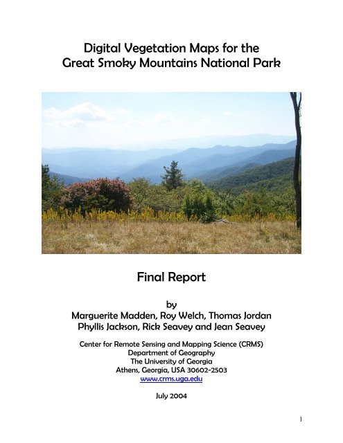
Digital <strong>Vegetation</strong> Maps for <strong>the</strong><br />
Great Smoky Mountains National Park<br />
Final <strong>Report</strong><br />
by<br />
Marguerite Madden, Roy Welch, Thomas Jordan<br />
Phyllis Jackson, Rick Seavey <strong>and</strong> Jean Seavey<br />
Center for Remote Sensing <strong>and</strong> <strong>Mapping</strong> Science (CRMS)<br />
Department of Geography<br />
The University of Georgia<br />
A<strong>the</strong>ns, Georgia, USA 30602-2503<br />
www.crms.uga.edu<br />
July 2004<br />
1
Digital <strong>Vegetation</strong> Maps for <strong>the</strong><br />
Great Smoky Mountains National Park<br />
Final <strong>Report</strong><br />
by<br />
Marguerite Madden, Roy Welch, Thomas Jordan,<br />
Phyllis Jackson, Rick Seavey <strong>and</strong> Jean Seavey<br />
Center for Remote Sensing <strong>and</strong> <strong>Mapping</strong> Science (CRMS)<br />
Department of Geography<br />
The University of Georgia<br />
A<strong>the</strong>ns, Georgia, USA 30602-2503<br />
mmadden@uga.edu<br />
Submitted to:<br />
U.S. Department of Interior<br />
National Park Service<br />
Great Smoky Mountains National Park<br />
Gatlinburg, Tennessee<br />
Cooperative Agreement No.<br />
1443-CA-5460-98-019<br />
July 15, 2004<br />
2
Table of Contents<br />
Page<br />
List of Figures 4<br />
List of Tables 6<br />
List of Attachments 7<br />
Summary 8<br />
Introduction 8<br />
Study Area 10<br />
Methodology 12<br />
Photogrammetric Operations 15<br />
Photointerpretation Operations 17<br />
Overstory <strong>and</strong> Understory <strong>Vegetation</strong> Database <strong>and</strong> Map Products 22<br />
Modeling Applications 29<br />
Fire Fuel Modeling 29<br />
Percent Canopy Data Layers 34<br />
Understory Density 37<br />
Conclusion 38<br />
Acknowledgements 40<br />
References 41<br />
Attachments 45<br />
3
List of Figures<br />
Figure Description Page<br />
Figure 1. Location of (a) Appalachian Mountains <strong>and</strong> (b) Great Smoky 9<br />
Mountains National Park in eastern United States.<br />
Figure 2. 3D perspective view of GRSM constructed from a mosaic of SPOT 11<br />
multispectral images draped over a digital elevation model. Elevations<br />
range from approximately 200 to over 2000 m above sea level.<br />
Figure 3. An example of a large-scale color infrared aerial photograph recorded 12<br />
in October 1997 <strong>and</strong> used for photo interpretation of vegetation detail.<br />
Figure 4. Diagram showing photogrammetric, photointerpretation <strong>and</strong> GIS 14<br />
operations used to map <strong>the</strong> vegetation of GRSM.<br />
Figure 5. Tree tops were used as pass points in overlapping images in <strong>the</strong> 16<br />
heavily forested GRSM.<br />
Figure 6. The elevations of ground control points (GCPs) were determined from 16<br />
<strong>the</strong> 30-m digital elevation model (DEM) using bilinear interpolation.<br />
Figure 7. A mosaic of orthorectified 1:12,000-scale photographs was created 17<br />
for quality assurance <strong>and</strong> checking.<br />
Figure 8. Ground digital image of overstory <strong>and</strong> understory vegetation recorded 18<br />
with a Kodak FIS 265 digital camera interfaced to a Garmin III Plus GPS.<br />
Figure 9. (a) Original photo overlay depicting vegetation polygons <strong>and</strong> a 1-cm grid 21<br />
before corrections for relief displacement. (b) Overlay <strong>and</strong> grid after<br />
orthorectification showing <strong>the</strong> extreme corrections required to accommodate<br />
<strong>the</strong> large range of relief in <strong>the</strong> area.<br />
Figure 10. Individual vector files from four adjacent photos that have been edited 22<br />
<strong>and</strong> edge matched.<br />
Figure 11. Hardcopy vegetation maps plotted at 1:15,000 scale correspond to <strong>the</strong> area 23<br />
covered by 25 individual <strong>USGS</strong> 7.5-minute topographic quadrangles in<br />
GRSM as outlined on this generalized overview map of GRSM overstory<br />
vegetation.<br />
4
List of Figures (Continued)<br />
Figure Description Page<br />
Figure 12. Generalized overview map of GRSM understory vegetation. 24<br />
Figure 13. Total area (hectares) of generalized overstory vegetation classes in GRSM. 27<br />
Figure 14. Total area (hectares) of generalized understory vegetation classes in GRSM. 28<br />
Figure 15. National Park Service resource/fire managers Mike Jenkins <strong>and</strong> Leon Konz, 30<br />
along with CRMS research assistant, Robin (Dukes) Puppa, determine <strong>the</strong><br />
Anderson Fuel Model associated with a particular vegetation community in<br />
GRSM.<br />
Figure 16. Examples of GRSM vegetation communities associated with Anderson Fuel 31, 32<br />
Models.<br />
Figure 17. A sample of <strong>the</strong> fire fuel model data set with fuel model values based on 35<br />
unique combinations of overstory/understory vegetation <strong>and</strong> understory<br />
density (decimals).<br />
Figure 18. CRMS photo interpreter Phyllis Jackson <strong>and</strong> NatureServe botanists Alan 35<br />
Weakly <strong>and</strong> Rickie White assess <strong>the</strong> vegetation community <strong>and</strong> percent<br />
canopy in <strong>the</strong> field.<br />
Figure 19. Percent canopy within <strong>the</strong> Gatlinburg quadrangle in leaf-on (a) <strong>and</strong> 36<br />
leaf-off (b) conditions color-coded according to canopy classes based on<br />
percent of canopy closure (c).<br />
Figure 20. A portion of <strong>the</strong> GRSM understory density data set depicting light, medium 38<br />
<strong>and</strong> heavy densities of Rhododendron (R), Kalmia (K) <strong>and</strong> mixed<br />
Rhododendron/Kalmia (RK).<br />
5
List of Tables<br />
Table Description Page<br />
Table 1. Specifications of data sources available for map/database development 13<br />
of GRSM.<br />
Table 2. Sample hierarchy of alpine forest classes within <strong>the</strong> overstory vegetation 19<br />
classification system for GRSM cross referenced to association descriptions<br />
by CEGL numbers in <strong>the</strong> National <strong>Vegetation</strong> <strong>Classification</strong> System.<br />
Table 3. Sample classes within <strong>the</strong> understory vegetation classification system 20<br />
for GRSM.<br />
Table 4. Generalized overstory vegetation <strong>and</strong> area statistics for GRSM. 26<br />
Table 5. Generalized understory vegetation <strong>and</strong> area statistics for GRSM. 28<br />
Table 6. Level I rules for assigning fuel classes in GRSM. 33<br />
Table 7. Example of Level II rules for assigning decimal values to fuel classes. 33<br />
Table 8. Percent canopy classes. 34<br />
6
List of Attachments<br />
Attachment<br />
Attachment A<br />
Attachment B<br />
Attachment C<br />
Attachment D<br />
Attachment E<br />
Attachment F<br />
Attachment G<br />
Attachment H<br />
Description<br />
Reprint of Jordan (2004), Control extension <strong>and</strong> orthorectification<br />
procedures for compiling vegetations databases of National Parks<br />
in <strong>the</strong> Sou<strong>the</strong>astern United States, In, M.O. Altan, Ed., International<br />
Archives of Photogrammetry <strong>and</strong> Remote Sensing, Vol. 35,<br />
Part 4B: 422-428.<br />
CRMS-NatureServe Overstory <strong>Vegetation</strong> <strong>Classification</strong> System<br />
for mapping Great Smoky Mountains National Park, by Phyllis Jackson,<br />
Rickie White <strong>and</strong> Marguerite Madden.<br />
Details on <strong>the</strong> CRMS-NatureServe Overstory GRSM <strong>Vegetation</strong><br />
<strong>Classification</strong> System, by Phyllis Jackson.<br />
CRMS Understory <strong>Vegetation</strong> <strong>Classification</strong> System for mapping<br />
Great Smoky Mountains National Park, by Rick Seavey <strong>and</strong> Jean Seavey.<br />
Details on <strong>the</strong> CRMS GRSM Understory <strong>Vegetation</strong> <strong>Classification</strong><br />
System, by Rick Seavey <strong>and</strong> Jean Seavey.<br />
Summary of Park-wide statistics for overstory classes.<br />
Summary of Park-wide statistics for understory classes.<br />
Reprint of Madden (2004) <strong>Vegetation</strong> modeling, analysis <strong>and</strong> visualization in<br />
U.S. National Parks, In, M.O. Altan, Ed., International Archives of<br />
Photogrammetry <strong>and</strong> Remote Sensing, Vol. 35, Part 4B: 1287-1292.<br />
7
Digital <strong>Vegetation</strong> Maps for <strong>the</strong><br />
Great Smoky Mountains National Park<br />
Summary<br />
Detailed overstory <strong>and</strong> understory vegetation, forest fire fuels, percent canopy <strong>and</strong> understory<br />
density databases <strong>and</strong> associated maps of <strong>the</strong> 2000 km 2 Great Smoky Mountains National Park<br />
were developed by <strong>the</strong> Center for Remote Sensing <strong>and</strong> <strong>Mapping</strong> Science at The University of<br />
Georgia in support of resource management activities of <strong>the</strong> U.S. National Park Service.<br />
Overstory vegetation was identified to <strong>the</strong> association level <strong>and</strong> crosswalked to <strong>the</strong> finest<br />
division of <strong>the</strong> National <strong>Vegetation</strong> <strong>Classification</strong> System (NVCS) protocol for <strong>the</strong> U.S.<br />
Geological Survey (<strong>USGS</strong>) – National Park Service (NPS) <strong>Vegetation</strong> <strong>Mapping</strong> Program.<br />
Understory vegetation was identified using an association-level classification system developed<br />
in this project that included density estimates when possible. With terrain relief exceeding 1700<br />
m <strong>and</strong> continuous forest cover over 95 percent of <strong>the</strong> Park, <strong>the</strong> requirement to use 1:12,000 <strong>and</strong><br />
1:40,000-scale color infrared aerial photographs as <strong>the</strong> primary data source for vegetation<br />
interpretation created a photogrammetric challenge. Challenges included lack of suitable ground<br />
control, excessive relief displacements <strong>and</strong> over 1000 photographs needed to cover <strong>the</strong> study<br />
area. In addition, Great Smoky Mountains National Park contains <strong>the</strong> world’s most botanically<br />
diverse temperature zone forest <strong>and</strong> required <strong>the</strong> creation of a detailed, hierarchical classification<br />
system. For <strong>the</strong>se reasons, a combination of analog photointerpretation, digital softcopy<br />
photogrammetry, geographic information system (GIS) <strong>and</strong> Global Positioning System (GPS)-<br />
assisted field data collection procedures were employed in <strong>the</strong> construction of <strong>the</strong> vegetation<br />
databases. Once complete, <strong>the</strong> overstory <strong>and</strong> understory vegetation databases were input to rulebased<br />
GIS models for analysis of forest fire fuels, percent canopy <strong>and</strong> understory density. All<br />
toge<strong>the</strong>r, <strong>the</strong> overstory <strong>and</strong> understory vegetation data sets total 513 mb of digital data, while fire<br />
products of fuel model classes, leaf-on percent canopy, leaf-off percent canopy <strong>and</strong> understory<br />
density total 605 Mb. Hardcopy maps tiled by U.S. Geological Survey (<strong>USGS</strong>) 7.5-minute<br />
topographic quadrangle (all or portions of 25 quads are contained in GRSM) were plotted at<br />
1:15,000 scale for overstory <strong>and</strong> understory vegetation. These maps depict <strong>the</strong> full detail of <strong>the</strong><br />
170 <strong>and</strong> 196 unique, association-level classes in <strong>the</strong> overstory <strong>and</strong> understory, respectively. The<br />
overstory database contains nearly 50,000 polygons (513 Mb of data) <strong>and</strong> <strong>the</strong> understory<br />
database contains nearly 25,500 polygons (605 Mb). Generalized overstory <strong>and</strong> understory<br />
vegetation data sets with approximately 24 classes each were created using GIS reclassification<br />
comm<strong>and</strong>s <strong>and</strong> used to produce 1:80,000-scale overview maps of <strong>the</strong> entire park. Fire fuel<br />
model, percent canopy (leaf-on <strong>and</strong> leaf-off) <strong>and</strong> understory density data sets also were used to<br />
produce park-wide maps.<br />
Introduction<br />
Great Smoky Mountains National Park (GRSM) encompasses approximately 2,000 km 2 of<br />
continuous forest cover in <strong>the</strong> sou<strong>the</strong>rn Appalachian Mountains in sou<strong>the</strong>astern United States<br />
(Figure 1). Located along <strong>the</strong> North Carolina-Tennessee border, this national park receives as<br />
many as 10 million visitors each year, yet contains one of <strong>the</strong> most diverse collections of plants<br />
8
<strong>and</strong> animals in <strong>the</strong> world. It has been designated as both an International Biosphere Reserve <strong>and</strong><br />
a World Heritage Site (Walker, 1991).<br />
a.<br />
b.<br />
Figure 1. Location of (a) Appalachian Mountains <strong>and</strong> (b) Great Smoky Mountains National Park<br />
in eastern United States.<br />
Although <strong>the</strong> GRSM was mapped at 1:24,000 scale by <strong>the</strong> U.S. Geological Survey (<strong>USGS</strong>) in<br />
<strong>the</strong> 1960s <strong>and</strong> 1970s, <strong>the</strong>se topographic maps, while essential, do not provide <strong>the</strong> detailed<br />
information <strong>and</strong> flexibility required to manage <strong>the</strong> Park, protect it from threats due to fire <strong>and</strong><br />
9
population pressure, or to monitor changes caused by air pollution <strong>and</strong> invasive exotic plants <strong>and</strong><br />
animals. These problems at GRSM <strong>and</strong> o<strong>the</strong>r parks have led <strong>the</strong> <strong>USGS</strong> <strong>and</strong> <strong>the</strong> National Park<br />
Service (NPS) to sponsor <strong>the</strong> development of detailed vegetation databases in digital format from<br />
remotely sensed data that can be used in a geographic information system (GIS) environment to<br />
create large-scale map products, conduct analyses of change <strong>and</strong> support <strong>the</strong> preservation of our<br />
national resources (<strong>USGS</strong>, 2002). The <strong>USGS</strong>-NPS National <strong>Vegetation</strong> <strong>Mapping</strong> Program aims<br />
to map all of <strong>the</strong> National Park System units using a consistent vegetation classification system<br />
<strong>and</strong> mapping protocol (Grossman et al. 1994, 1998; Maybury 1999).<br />
The Center for Remote Sensing <strong>and</strong> <strong>Mapping</strong> Science (CRMS), Department of Geography at<br />
The University of Georgia, (www.crms.uga.edu) has been involved in vegetation mapping <strong>and</strong><br />
database development in national parks of <strong>the</strong> sou<strong>the</strong>astern U.S. for <strong>the</strong> past 10 years (Welch et<br />
al. 1995, 1999, 2002a, 2002b; Welch <strong>and</strong> Remillard 1996). As a remote sensing <strong>and</strong> mapping<br />
facility, <strong>the</strong> CRMS is unique in is combination of expertise in both technical <strong>and</strong> biological<br />
aspects of vegetation mapping projects. Scientists at <strong>the</strong> CRMS specialize in image processing,<br />
photogrammetry, GIS, air photo interpretation <strong>and</strong> field surveying, as well as botany, biology<br />
<strong>and</strong> ecology. This allows a close link between <strong>the</strong> two major components of a vegetation<br />
mapping/database project: 1) photogrammetric rectification <strong>and</strong> GIS database construction; <strong>and</strong><br />
2) vegetation interpretation, classification <strong>and</strong> field verification.<br />
In addition to in-house cross training of technical <strong>and</strong> biological skills, <strong>the</strong> CRMS has<br />
developed a strong working relationship with NatureServe, a non-profit conservation<br />
organization that developed <strong>the</strong> U.S. National <strong>Vegetation</strong> <strong>Classification</strong> System <strong>and</strong> is a primary<br />
partner in <strong>the</strong> <strong>USGS</strong>-NPS <strong>Vegetation</strong> <strong>Mapping</strong> Program (www.natureserve.org). Collaboration<br />
between <strong>the</strong> CRMS <strong>and</strong> <strong>the</strong> NatureServe-Durham, North Carolina Office has resulted in <strong>the</strong><br />
development of a detailed classification system for GRSM that maximizes <strong>the</strong> information on<br />
vegetation communities that can be gleaned from large-scale color infrared aerial photographs,<br />
while remaining compatible with <strong>the</strong> U.S. National <strong>Vegetation</strong> <strong>Classification</strong> System (Anderson<br />
et al. 1998, Jackson et al. 2002).<br />
The objectives of this report are to: 1) demonstrate how digital photogrammetry,<br />
photointerpretation, GIS <strong>and</strong> Global Positioning Systems (GPS)-assisted field techniques were<br />
refined, adapted <strong>and</strong> integrated to permit <strong>the</strong> construction of geocoded vegetation databases from<br />
more than 1,000 large-scale aerial photographs of <strong>the</strong> rugged, high-relief GRSM; 2) discuss <strong>the</strong><br />
CRMS-NatureServe GRSM <strong>Vegetation</strong> <strong>Classification</strong> System; <strong>and</strong> 3) present GIS analyses of<br />
<strong>the</strong> overstory <strong>and</strong> understory vegetation databases for <strong>the</strong> development of fuel models, percent<br />
cover <strong>and</strong> understory density for <strong>the</strong> management <strong>and</strong> control of forest fires. Because GRSM is<br />
considered one of <strong>the</strong> most difficult terrain areas to map in <strong>the</strong> United States, it is envisioned that<br />
<strong>the</strong> techniques discussed below can be modified as necessary <strong>and</strong> applied to rugged <strong>and</strong> remote,<br />
forested l<strong>and</strong>s in o<strong>the</strong>r U.S. National Parks.<br />
Study Area<br />
Great Smoky Mountains National Park was established in 1934 in an attempt to halt <strong>the</strong><br />
damage to forests caused by erosion <strong>and</strong> fires associated with logging activities of <strong>the</strong> 1800s <strong>and</strong><br />
early 1900s. By <strong>the</strong> 1920s, nearly two-thirds of <strong>the</strong> l<strong>and</strong>s that would become GRSM had been<br />
10
logged or burned (Walker, 1991). The Park now protects 2000 km 2 of forestl<strong>and</strong> within <strong>the</strong><br />
sou<strong>the</strong>rn Appalachian Mountains – among <strong>the</strong> oldest mountain ranges on earth. Elevations in<br />
GRSM range from approximately 250 m along <strong>the</strong> outside boundary of <strong>the</strong> Park to 2,025 m at<br />
Clingman’s Dome (Figure 2). Rock formations in <strong>the</strong> region are sedimentary, <strong>the</strong> result of silt,<br />
s<strong>and</strong> <strong>and</strong> gravel deposits into a shallow sea that covered <strong>the</strong> area between 900 <strong>and</strong> 600 million<br />
years ago (Moore, 1988). More than 900 km of streams <strong>and</strong> rivers that flow within <strong>the</strong> Park are<br />
replenished by over 200 cm of rain per year. As of 2004, 1,637 species (1,293 native <strong>and</strong> 344<br />
exotic) of flowering plants, 10 percent of which are considered rare, <strong>and</strong> over 4,000 species of<br />
non-flowering plants are found in GRSM (Walker, 1991). The forestl<strong>and</strong>s include over 100<br />
different species of trees <strong>and</strong> contain <strong>the</strong> most extensive virgin hardwood forest in <strong>the</strong> eastern<br />
United States (Whittaker, 1956; Kemp, 1993; Houk, 2000).<br />
Figure 2. 3D perspective view of GRSM constructed from a mosaic of SPOT multispectral<br />
images draped over a digital elevation model. Elevations range from approximately 200 to over<br />
2000 m above sea level.<br />
Scientists estimate that <strong>the</strong> flora <strong>and</strong> fauna currently identified in <strong>the</strong> Park represent only 10<br />
percent of <strong>the</strong> total species that are likely present (Kaiser, 1999). In order to discover <strong>the</strong> full<br />
range of life in GRSM, an ambitious project is underway known as <strong>the</strong> All Taxa Biodiversity<br />
Inventory (ATBI) that aims to identify every life form in <strong>the</strong> Park (possibly over 100,000<br />
species) over <strong>the</strong> next ten to fifteen years (White <strong>and</strong> Morse, 2000). The efforts of ATBI<br />
participants rely heavily on map information in order to locate various habitats, conduct<br />
fieldwork <strong>and</strong> establish sample plots.<br />
Natural resource managers at GRSM realized early-on <strong>the</strong> value of producing a detailed<br />
vegetation database that could be used to map habitats <strong>and</strong> aid researchers in <strong>the</strong>ir quest for<br />
identifying new mountain species. They also required a vegetation database for providing<br />
baseline information for future monitoring <strong>and</strong> management tasks. Facing threats by air<br />
pollution, invasive exotic plants <strong>and</strong> animals such as <strong>the</strong> hemlock woolly adelgid (Adelges<br />
11
tsugae), large numbers of Park visitors, arson/accidental forest fires <strong>and</strong> exotic diseases (e.g.,<br />
chestnut blight, dogwood anthracnose, beech bark disease, butternut canker <strong>and</strong>, potentially,<br />
sudden oak death), Park managers needed analysis tools to assist <strong>the</strong>m in <strong>the</strong> preservation of<br />
valuable resources. Consequently, in 1999, <strong>the</strong> Center for Remote Sensing <strong>and</strong> <strong>Mapping</strong> Science<br />
at The University of Georgia entered into a Cooperative Agreement with <strong>the</strong> NPS to create a<br />
detailed digital database for GRSM that includes both overstory <strong>and</strong> understory vegetation <strong>and</strong><br />
an analysis of fuels that can cause forest fires in <strong>the</strong> Park.<br />
Methodology<br />
The main requirement for <strong>the</strong> project was to produce a vegetation database <strong>and</strong> associated<br />
maps in vector format that contained polygons for over 150 overstory <strong>and</strong> understory plant<br />
communities plotted to within approximately + 5 to + 10 m of <strong>the</strong>ir true ground locations.<br />
Overstory vegetation was mapped using more than 1000 color infrared aerial photographs of<br />
1:12,000 scale in film transparency format recorded with a Wild RC20 photogrammetric camera,<br />
f = 15 cm) in late October by <strong>the</strong> U. S. Forest Service. The fall photos were acquired when <strong>the</strong><br />
leaves were still on <strong>the</strong> trees (leaf-on) <strong>and</strong> displayed a color diversity that allowed <strong>the</strong> vegetation<br />
communities/species to be identified (Table 1, Figure 3). Relief displacements were a major<br />
problem, in some cases reaching more than 40 mm on <strong>the</strong> 23 x 23 cm format photographs<br />
(Jordan, 2004; Attachment A).<br />
Figure 3. An example of a large-scale color infrared aerial photograph recorded in October 1997<br />
<strong>and</strong> used for photo interpretation of vegetation detail.<br />
12
The understory vegetation was mapped from 1:40,000-scale color infrared photographs recorded<br />
(with a Wild RC30 camera, f = 15 cm) in <strong>the</strong> winter months as part of <strong>the</strong> <strong>USGS</strong> National Aerial<br />
Photography Program (NAPP). At that time of year, deciduous trees have lost <strong>the</strong>ir leaves (leafoff)<br />
<strong>and</strong> it is possible to delineate <strong>the</strong> understory evergreen shrubs <strong>and</strong> trees that are both<br />
combustible <strong>and</strong> sufficiently dense to restrict crews combating forest fires or conducting search<br />
<strong>and</strong> rescue missions. With <strong>the</strong> dense forest cover, steep slopes, absence of ground control <strong>and</strong><br />
relief exceeding 30 percent of <strong>the</strong> flying height for <strong>the</strong> large-scale photographic coverage, <strong>the</strong><br />
construction of a vegetation database accurate in both <strong>the</strong> spatial <strong>and</strong> <strong>the</strong>matic context<br />
necessitated a combination of softcopy photogrammetry, photointerpretation <strong>and</strong> GIS procedures<br />
organized in parallel as shown in Figure 4. These are discussed below.<br />
Table 1. Specifications of data sources available for map/database development of GRSM.<br />
Data Source Format <strong>and</strong> Flying Resoluti No. Comments <strong>and</strong>/or<br />
Type of Height (FH) on Required Problems<br />
Data <strong>and</strong>/or Scale to Cover<br />
<strong>the</strong> Park<br />
Color infrared 23 x 23 cm FH =1800 m Terrain relief in excess of<br />
(CIR) Air Photos<br />
30% of flying height. A<br />
Analog film 1:12,000 ~ 0.4 m ~ 1,000 smaller scale could<br />
October 1997- transparencies alleviate this problem. Fall<br />
1998 leaf-on conditions are ideal<br />
for mapping overstory<br />
forest communities.<br />
<strong>USGS</strong> NAPP Air 23 x 23 cm FH ≈ 6,000 m Scale is too small for<br />
Photos<br />
mapping overstory<br />
Analog film 1:40,000 ~ 1m ~ 130 vegetation. Leaf-off<br />
March/April 1997- transparencies conditions are ideal for<br />
1998 mapping understory<br />
vegetation.<br />
<strong>USGS</strong> Paper maps 1:24,000 - 25 Last updated 1960-1970’s.<br />
Topographic Maps<br />
<strong>USGS</strong> DOQQs Digital - 1 m 80 <strong>USGS</strong> DOQQs have a<br />
planimetric accuracy of<br />
Pan <strong>and</strong> CIR<br />
approximately ± 3 m RMS.<br />
<strong>USGS</strong> Level 2 Digital 1:24,000 30 m post 25 <strong>USGS</strong> Level 2 DEMs have<br />
DEMs spacing a vertical accuracy of<br />
approximately ± 3-5 m<br />
RMS.<br />
13
Figure 4. Diagram showing photogrammetric, photointerpretation <strong>and</strong> GIS operations used to<br />
map <strong>the</strong> vegetation of GRSM.<br />
14
Photogrammetric Operations<br />
The main objective of <strong>the</strong> photogrammetric procedure was to densify <strong>the</strong> sparse ground<br />
control in <strong>the</strong> Park by means of aerotriangulation, a photogrammetric operation whereby a<br />
relatively small number of ground control points (GCPs) are used to ma<strong>the</strong>matically compute <strong>the</strong><br />
ground coordinates of a much larger number of identified pass points (Jordan, 2002). In this<br />
way, <strong>the</strong> control network is adequately densified for <strong>the</strong> orthorectification process. At <strong>the</strong> outset,<br />
<strong>the</strong> 1:12,000-scale film transparencies were scanned at 600 dots per inch (dpi) using an Epson<br />
Expression 836xl desktop scanner to create black-<strong>and</strong>-white digital photos of 42-µm pixel<br />
resolution, providing a file of 35 Mbytes for each photo. These digital photos were <strong>the</strong>n<br />
displayed on <strong>the</strong> computer monitor <strong>and</strong> with <strong>the</strong> aid of <strong>the</strong> R-WEL, Inc. Desktop <strong>Mapping</strong><br />
System (DMS) software package, <strong>the</strong> image (x,y) coordinates of pass points <strong>and</strong> GCPs were<br />
measured in <strong>the</strong> softcopy environment. This was a painstaking <strong>and</strong> time-consuming task. In <strong>the</strong><br />
absence of cultural features <strong>and</strong> <strong>the</strong> near continuous tree canopy cover, <strong>the</strong> passpoints, in <strong>the</strong><br />
majority of instances, were individual tree-tops that had to be identified uniquely on overlapping<br />
photographs – not an easy job in terrain of high relief recorded on large-scale photographs<br />
(Figure 5).<br />
Ground control points were, for <strong>the</strong> most part, natural features (e.g., rock outcrops <strong>and</strong> forks<br />
in stream channels) identified on both <strong>the</strong> 1:12,000-scale color infrared transparencies <strong>and</strong> <strong>USGS</strong><br />
Digital Orthophoto Quarter Quads (DOQQs) produced from 1:40,000-scale panchromatic aerial<br />
photographs recorded in 1993. The Universal Transverse Mercator (UTM) grid coordinates<br />
(X,Y tied to <strong>the</strong> North American Datum of 1927 or NAD 27) of <strong>the</strong>se GCPs were measured<br />
directly from <strong>the</strong> DOQQs (accurate to within + 3 m). Elevations for <strong>the</strong> GCPs were derived<br />
using CRMS custom software to interpolate <strong>the</strong> Z-coordinates to within + 3 to + 5 m from <strong>USGS</strong><br />
Level 2 Digital Elevation Models (DEMs) with 30-m post spacing (Figure 6). Thus, in this<br />
project, no ground survey work was required to obtain <strong>the</strong> GCPs needed as a framework for <strong>the</strong><br />
aerotriangulation process.<br />
Analytical aerotriangulation was undertaken for blocks of up to 90 photos, where each block<br />
corresponded to <strong>the</strong> area covered by one of <strong>the</strong> 25 <strong>USGS</strong> 1:24,000-scale map sheets covering <strong>the</strong><br />
Park. The PC Giant software package, in conjunction with <strong>the</strong> DMS software, was employed for<br />
<strong>the</strong> aerotriangulation process. Output from <strong>the</strong> aerotriangulation was a set of X, Y <strong>and</strong> Z<br />
coordinates in <strong>the</strong> UTM coordinate system for <strong>the</strong> nine or more pass points identified by CRMS<br />
personnel on each photo. Typical root-mean-square error (RMSE) values for <strong>the</strong>se coordinates<br />
averaged + 7 m for <strong>the</strong> XY vectors <strong>and</strong> + 10 m for elevations (Z).<br />
The pass points with <strong>the</strong>ir X, Y <strong>and</strong> Z coordinates derived from <strong>the</strong> aerotriangulation process<br />
provided <strong>the</strong> ground control required to generate orthophotos <strong>and</strong> mosaics from <strong>the</strong> scanned air<br />
photos (Figure 7). These orthophotos <strong>and</strong> mosaics, in turn, were employed in <strong>the</strong> editing <strong>and</strong><br />
attributing operations required to build <strong>the</strong> vector database. Most importantly, however, <strong>the</strong><br />
control provided by <strong>the</strong> aerotriangulation process was essential for rectifying vector overlays<br />
generated as part of <strong>the</strong> photointerpretation procedure described below.<br />
15
Figure 5. Tree tops were used as pass points in overlapping images in <strong>the</strong> heavily forested<br />
GRSM.<br />
3546789<br />
351 353<br />
GCP<br />
355.3<br />
355 360<br />
485367<br />
Figure 6. The elevations of ground control points (GCPs) were determined from <strong>the</strong> 30-m digital<br />
elevation model (DEM) using a bilinear interpolation algorithm.<br />
16
Figure 7. A mosaic of orthorectified 1:12,000-scale photographs was created for quality<br />
assurance <strong>and</strong> checking. Terrain features that are well aligned between individual photographs<br />
indicate a good overall solution. This is necessary for <strong>the</strong> rectified vegetation linework of<br />
individual photographs to edgematch correctly.<br />
Photointerpretation Operations<br />
The steps of <strong>the</strong> photointerpretation process listed in Figure 4 proceeded in parallel with <strong>the</strong><br />
photogrammetric operations. Overstory vegetation was interpreted from <strong>the</strong> 1:12,000-scale leafon<br />
color infrared aerial photographs. On <strong>the</strong> o<strong>the</strong>r h<strong>and</strong>, <strong>the</strong> understory vegetation was<br />
interpreted from <strong>the</strong> 1:40,000-scale (leaf-off) transparencies.<br />
Although it might appear desirable to scan <strong>the</strong> color infrared transparencies at high resolution<br />
<strong>and</strong> undertake <strong>the</strong> vegetation classification as an on-screen interpretation <strong>and</strong> digitizing<br />
procedure, this has proved to be exceedingly time consuming, cumbersome <strong>and</strong> expensive<br />
compared to more traditional approaches (Welch et al. 1995 <strong>and</strong> 1999; Rutchey <strong>and</strong> Vilchek<br />
1999). Moreover, photointerpreters must view <strong>the</strong> vegetation in stereo <strong>and</strong> in color within <strong>the</strong><br />
context of a relatively large area of terrain in order to identify <strong>the</strong> vegetation communities. This<br />
is most easily done using a stereoscope to view <strong>the</strong> analog air photos so that <strong>the</strong> vegetation<br />
17
patterns can be assessed in relation to <strong>the</strong> terrain. Recognizing <strong>the</strong> need to augment manual<br />
procedures with automated techniques, <strong>the</strong> steps described below integrate conventional<br />
photointerpretation procedures with digital processing technology in an attempt to streamline <strong>the</strong><br />
database <strong>and</strong> map compilation process.<br />
At <strong>the</strong> beginning of <strong>the</strong> GRSM mapping project, <strong>the</strong> photointerpreters, in conjunction with<br />
NPS plant specialists, conducted field investigations to collect data on <strong>the</strong> forest communities<br />
<strong>and</strong> correlate signatures evident on <strong>the</strong> aerial photographs with ground observations.<br />
Consequently, UTM coordinates <strong>and</strong> field data were collected at over 2000 locations with <strong>the</strong> aid<br />
of a Garmin III Plus h<strong>and</strong>-held GPS receiver <strong>and</strong> a Kodak Digital Field Imaging System (FIS)<br />
265 digital camera system. The h<strong>and</strong>-held Kodak digital camera was connected to <strong>the</strong> Garmin<br />
GPS that “stamped” <strong>the</strong> location, date <strong>and</strong> time on each image (Figure 8). These images were<br />
input to ArcView to provide a pictorial record of field observations.<br />
Figure 8. Ground digital image of overstory <strong>and</strong> understory vegetation recorded with a Kodak<br />
FIS 265 digital camera interfaced to a Garmin III Plus GPS.<br />
A compilation of all field information was used by Center for Remote Sensing <strong>and</strong> <strong>Mapping</strong><br />
Science (CRMS) ecologists to organize <strong>the</strong> GRSM overstory <strong>and</strong> understory vegetation into a<br />
classification system with 170 unique association-level classes suitable for use with <strong>the</strong> large <strong>and</strong><br />
medium-scale (1:12,000 <strong>and</strong> 1:40,000, respectively) color infrared aerial photographs (Jackson et<br />
al. 2002; Table 2). The term, association, is defined by Grossman et al. (1998) as a “plant<br />
community type of definite floristic composition, uniform habitat conditions <strong>and</strong> uniform<br />
physiognomy”. Terrestrial communities in GRSM have one to several strata of vegetation: tree<br />
canopy, sub-canopy, tall shrub, short shrub, herbaceous, non-vascular, vine/liana <strong>and</strong> epiphyte.<br />
The combination of vegetation in all of <strong>the</strong>se strata present determines <strong>the</strong> community type.<br />
18
The term “overstory vegetation” refers to <strong>the</strong> entire vegetation community. Communities are<br />
named <strong>and</strong> referenced by vegetation in <strong>the</strong>ir tallest stratum, plus abundant <strong>and</strong>/or indicator<br />
species in lower strata. Photointerpreters can see <strong>the</strong> tallest strata on color infrared photos, <strong>and</strong><br />
may or may not be able to see through this layer to shorter layers. Sometimes a community can<br />
be determined solely by seeing its location <strong>and</strong> seeing <strong>the</strong> uppermost stratum, for example, a<br />
Hardwood Cove. In o<strong>the</strong>r cases, a lower stratum (or strata) must be seen because this stratum<br />
determines <strong>the</strong> community type. For example, three kinds of Montane Red Oak communities<br />
have <strong>the</strong> same canopy, but <strong>the</strong>ir differences are determined by an evergreen tall shrub stratum, a<br />
deciduous tall shrub stratum, or an orchard-like herbaceous stratum.<br />
The overstory classification system was based on <strong>the</strong> <strong>USGS</strong>-NPS <strong>Vegetation</strong> <strong>Classification</strong> of<br />
GRSM for <strong>the</strong> area corresponding to <strong>the</strong> Cades Cove <strong>and</strong> Mount Le Conte <strong>USGS</strong> topographic<br />
quadrangles developed by The Nature Conservancy (TNC) as part of <strong>the</strong> <strong>USGS</strong>-NPS <strong>Vegetation</strong><br />
<strong>Mapping</strong> Program (TNC, 1999). The full overstory CRMS/NatureServe GRSM <strong>Vegetation</strong><br />
<strong>Classification</strong> system is provided in Attachment B with a crosswalk to NVCS Community<br />
Element Global (CEGL) code numbers for association divisions. Fur<strong>the</strong>r details on <strong>the</strong><br />
development <strong>and</strong> use of <strong>the</strong> CRMS/NatureServe GRSM <strong>Vegetation</strong> <strong>Classification</strong> system are<br />
provided in Attachment C.<br />
Table 2. Sample hierarchy of alpine forest classes within <strong>the</strong> overstory vegetation classification<br />
system for GRSM cross referenced to association descriptions by CEGL numbers in <strong>the</strong> National<br />
<strong>Vegetation</strong> <strong>Classification</strong> System.<br />
_________________________________________________________________________<br />
FOREST<br />
GRSM Veg Code [CEGL Code]<br />
A. Sub Alpine Mesic Forest<br />
1. Fraser Fir (above 6000 ft.) F [6049, 6308]<br />
a. Formerly Fraser Fir (F) [6049, 6308]<br />
b. Fraser Fir/Deciduous Shrub-Herbaceous F/Sb [6049]<br />
c. Fraser Fir/Rhododendron F/R [6308]<br />
2. Red Spruce – Fraser Fir S-F*, S/F, F/S [7130, 7131]<br />
a. Red Spruce – Fraser Fir/Rhododendron S-F/R [7130]<br />
b. Red Spruce – Fraser Fir/Low Shrub-Herb S-F/Sb [7131]<br />
3. Red Spruce S [7130,7131]<br />
a. Red Spruce/Rhododendron (5000-6000 ft.) S/R [7130]<br />
b. Red Spruce/Sou<strong>the</strong>rn Mountain Cranberry- S/Sb [7131]<br />
Low Shrub/Herbaceous (5400-6200 ft.)<br />
4. Red Spruce – Yellow Birch – Nor<strong>the</strong>rn Hardwood S/NHxB [6256]<br />
5. Exposed Nor<strong>the</strong>rn Hardwood/Red Spruce NHxE/S [3893]<br />
6. Beech Gap NHxBe [6246, 6130]<br />
a. North Slope Tall Herb Type NHxBe/Hb [6246]<br />
b. South Slope Sedge Type NHxBe/G [6130]<br />
* Symbols: (-) designates a equal mix <strong>and</strong> (/) designates <strong>the</strong> first class listed is dominate (> 50<br />
percent) over <strong>the</strong> second class listed.<br />
_______________________________________________________________________<br />
19
In order to accommodate <strong>the</strong> complex vegetation patterns found in GRSM <strong>and</strong> generally<br />
maintain a minimum mapping unit of 0.5 ha, a three-tiered scheme was developed for attributing<br />
vegetation polygons, similar to that developed for an earlier project in <strong>the</strong> Everglades of south<br />
Florida (Madden et al. 1999). The three-tiered scheme allowed photointerpreters to annotate<br />
each polygon in <strong>the</strong> database with a primary or dominant vegetation class accounting for more<br />
than 50 percent of <strong>the</strong> vegetation in <strong>the</strong> polygon. Where appropriate, secondary <strong>and</strong> tertiary<br />
vegetation classes are added to describe mixed-plant communities within <strong>the</strong> polygon. Secondary<br />
<strong>and</strong> tertiary classes were especially useful for describing ecotones, <strong>and</strong> for polygons with a<br />
patchwork of communities below <strong>the</strong> minimum mapping unit size. See Attachment C for fur<strong>the</strong>r<br />
explanation of <strong>the</strong> three-tiered polygon attribution procedure.<br />
A separate classification system containing over 196 unique association-level classes was<br />
developed by CRMS photointerpreters in consultation with NPS resource managers to map <strong>the</strong><br />
understory vegetation (Table 3).<br />
Table 3. Sample classes within <strong>the</strong> understory vegetation classification system for GRSM.<br />
_______________________________________________________________________<br />
Pine overstory with Kalmia understory<br />
a. Pine dominant over high density Kalmia (PI/Kh)<br />
b. Pine dominant over medium density Kalmia (PI/Km)<br />
c. Pine dominant over low density Kalmia (PI/Kl)<br />
d. Pine dominant over possible Kalmia (PI/Kp)<br />
e. Pine dominant over implied Kalmia (PI/Ki)<br />
* Symbols: (/) designates <strong>the</strong> first class listed is dominate (> 50 percent) over <strong>the</strong> second class<br />
listed.<br />
The term “understory” denotes woody vegetation of medium height (3 to 5 m) that does not<br />
reach <strong>the</strong> forest canopy level. Understory classes of particular interest to fire managers included<br />
two evergreen, broad-leaf shrubs: rhododendron (Rhododendron spp.) <strong>and</strong> mountain laurel<br />
(Kalmia latifolia). Information on <strong>the</strong> location <strong>and</strong> density of <strong>the</strong>se understory shrubs is<br />
important for modeling fire fuels, assessing fire behavior <strong>and</strong> determining accessibility for<br />
research, resource management <strong>and</strong> search <strong>and</strong> rescue activities. Interpretation of <strong>the</strong>se<br />
understory vegetation strata from <strong>the</strong> air photos, <strong>the</strong>refore, included fur<strong>the</strong>r classification<br />
according to <strong>the</strong> density of <strong>the</strong> shrub as light (l), medium (m) or heavy (h). Additional<br />
subclasses were added for <strong>the</strong>se shrub areas of interest to qualify uncertainty in <strong>the</strong>ir<br />
interpretation <strong>and</strong> identification when <strong>the</strong> understory was obscured by overstory vegetation. In<br />
<strong>the</strong>se cases, <strong>the</strong> evergreen forest community (e.g., “T” for hemlock) <strong>and</strong> <strong>the</strong> probable understory<br />
shrub (e.g., “R” for rhododendron) are combined in a single label of T/R with an indicator of “i”<br />
to denote “implied” or “p” to denote “possible” rhododendron, in place of a density symbol (i.e.,<br />
T/Ri). Implied is defined to mean <strong>the</strong> conditions are right for <strong>the</strong> presence of <strong>the</strong> species <strong>and</strong> it<br />
is believed to be found <strong>the</strong>re. On <strong>the</strong> o<strong>the</strong>r h<strong>and</strong>, possible is defined as <strong>the</strong> conditions are only<br />
marginally right for <strong>the</strong> presence of <strong>the</strong> species. The full understory classification system is<br />
20
provided in Attachment D, <strong>and</strong> fur<strong>the</strong>r details on <strong>the</strong> development of <strong>the</strong> understory classification<br />
system <strong>and</strong> <strong>the</strong> interpretation of understory communities can be found in Attachment E.<br />
Once <strong>the</strong> overstory community <strong>and</strong> understory vegetation classification systems were<br />
established, <strong>the</strong> photointerpretation proceeded by taping transparent plastic overlays to <strong>the</strong> film<br />
transparencies, <strong>and</strong> transferring <strong>the</strong> photo numbers <strong>and</strong> fiducial marks to <strong>the</strong> overlays by means<br />
of a Rapidograph technical pen. The film transparencies, with plastic overlays, were <strong>the</strong>n placed<br />
on a high intensity light table <strong>and</strong> <strong>the</strong> polygons corresponding to <strong>the</strong> vegetation classes outlined<br />
on <strong>the</strong> overlay using <strong>the</strong> Rapidograph pen while viewing <strong>the</strong> photographs through a stereoscope.<br />
This is a simple, fast, inexpensive <strong>and</strong> flexible method of creating a vegetation overlay that can<br />
be scanned to create a raster file.<br />
Following recommendations by Welch <strong>and</strong> Jordan (1996), <strong>the</strong> scanning process involved <strong>the</strong><br />
use of <strong>the</strong> desktop Epson 836xl scanner, at a resolution of 42 µm (600 dpi). All annotated point,<br />
line <strong>and</strong> polygon information on <strong>the</strong> overlay was converted to raster format. The parameters<br />
derived from <strong>the</strong> differential rectification of <strong>the</strong> scanned 1:12,000-scale photos were applied to<br />
<strong>the</strong> scanned overlay files via registration with <strong>the</strong> transferred fiducial marks. Figure 9 illustrates<br />
<strong>the</strong> magnitude of polygon displacement, as well as distortion in polygon shape <strong>and</strong> size, due to<br />
variable relief displacements across <strong>the</strong> photograph.<br />
a. b.<br />
Figure 9. (a) Original photo overlay depicting vegetation polygons <strong>and</strong> a 1-cm grid before<br />
corrections for relief displacement. (b) Overlay <strong>and</strong> grid after orthorectification showing <strong>the</strong><br />
extreme corrections required to accommodate <strong>the</strong> large range of relief in <strong>the</strong> area.<br />
21
Overstory <strong>and</strong> Understory <strong>Vegetation</strong> Database <strong>and</strong> Map Products<br />
Upon differential rectification of <strong>the</strong> scanned raster overlay files, <strong>the</strong>se files are converted to<br />
vector format with <strong>the</strong> software package R2V by Able Software Company (Cambridge,<br />
Massachusetts) <strong>and</strong> saved in ArcInfo line format. Vector files from approximately 45<br />
photographs must be edited, edgematched <strong>and</strong> incorporated into a single ArcInfo coverage to<br />
produce one vegetation map corresponding to <strong>the</strong> area covered by a single <strong>USGS</strong> topographic<br />
quadrangle (Figure 10). A typical coverage for <strong>the</strong> area corresponding to a <strong>USGS</strong> 1:24,000-scale<br />
map can contain over 4,500 polygons that must be attributed with a dominant vegetation class,<br />
<strong>and</strong> possibly secondary <strong>and</strong> tertiary vegetation classes. More than 700 man-hours are required to<br />
produce a single quad-sized vegetation map from <strong>the</strong> 1:12,000-scale photos, including quality<br />
control checks of labels/line work within <strong>and</strong> between adjacent maps. Understory maps,<br />
produced from <strong>the</strong> smaller scale NAPP air photos, require approximately 100 man-hours to<br />
prepare. Although limited funds available for <strong>the</strong> project precluded a thorough check of<br />
<strong>the</strong>matic classification accuracy, maps were taken into <strong>the</strong> field as <strong>the</strong>y were completed to assess<br />
<strong>the</strong> general agreement between map information <strong>and</strong> observations on <strong>the</strong> ground.<br />
Figure 10. Individual vector files from four adjacent photos that have been edited <strong>and</strong> edge<br />
matched.<br />
Final products included a seamless GIS database in Arc/Info coverage <strong>and</strong> ArcView shapefile<br />
formats of detailed overstory <strong>and</strong> understory vegetation communities for <strong>the</strong> entire park, along<br />
with hardcopy maps plotted at 1:15,000 scale corresponding to <strong>the</strong> area covered by 25 individual<br />
<strong>USGS</strong> 7.5-minute topographic quadrangles (Figures 11 <strong>and</strong> 12). Each map sheet contains a<br />
color-coded legend <strong>and</strong> brief description of all vegetation classes found in GRSM. A<br />
demonstration of additional digital/hardcopy products that can be created for particular areas of<br />
interest as a result of <strong>the</strong> vegetation database development include color orthophoto mosaics <strong>and</strong><br />
drapes of maps/images on <strong>the</strong> DEM to enhance visualization of vegetation patterns with respect<br />
22
Figure 11. Hardcopy vegetation maps plotted at 1:15,000 scale correspond to <strong>the</strong> area covered by 25 individual <strong>USGS</strong> 7.5-minute topographic<br />
quadrangles in GRSM, as outlined on this generalized overview map of GRSM overstory vegetation.<br />
23
Figure 12. Generalized overview map of GRSM understory vegetation.<br />
24
to <strong>the</strong> terrain. Applications of <strong>the</strong> GRSM map/database products include: 1) vegetation<br />
assessment for general resource management tasks; <strong>and</strong> 2) utilization of <strong>the</strong> overstory <strong>and</strong><br />
understory vegetation structure for classifying fuels <strong>and</strong> <strong>the</strong> associated risk of forest fire.<br />
The overstory <strong>and</strong> understory databases provide a basis for park-wide resource management<br />
decisions. Basic information that is required by all managers includes a spatial inventory of<br />
existing vegetation communities <strong>and</strong> summary statistics indicating <strong>the</strong> total area covered by each<br />
community. These data can be quickly tallied in a GIS environment once <strong>the</strong> database has been<br />
developed. Attachments F <strong>and</strong> G contain a comprehensive list of all overstory <strong>and</strong> understory<br />
vegetation classes in <strong>the</strong> database <strong>and</strong> <strong>the</strong>ir respective areas within <strong>the</strong> park.<br />
Detailed information at <strong>the</strong> association-level is often needed to address management problems<br />
that target individual species. For example, <strong>the</strong> overstory vegetation database can be queried to<br />
locate pure st<strong>and</strong>s of high elevation table mountain pine (Pinus pungens) requiring controlled<br />
burning to eliminate hardwood invasion. Polygons containing Eastern hemlock (Tsuga<br />
canadensis) also can be reselected to identify areas susceptible to die-off <strong>and</strong> damage caused by<br />
<strong>the</strong> non-native hemlock woolly adelgid.<br />
O<strong>the</strong>r management questions may require a broader-perspective. Given <strong>the</strong> complexity of<br />
vegetation diversity in GRSM, it is difficult for managers to assess general trends in vegetation<br />
patterns when posed with management questions on a Park-wide level. The hierarchical<br />
structure of <strong>the</strong> GRSM <strong>Vegetation</strong> <strong>Classification</strong> System allows this to be easily accomplished.<br />
To this end, 170 association-level overstory vegetation classes were collapsed to 24 classes that<br />
approximate <strong>the</strong> alliance level of <strong>the</strong> National <strong>Vegetation</strong> <strong>Classification</strong> System (Table 4). A<br />
lookup table was used to reclassify <strong>the</strong> overstory attributes of polygons to <strong>the</strong> more general forest<br />
type classes <strong>and</strong> <strong>the</strong> Arc/Info Dissolve comm<strong>and</strong> was used to create new polygon boundaries<br />
surrounding <strong>the</strong> forest types (See attached CD for lookup table files). A composite map<br />
depicting generalized forest types for <strong>the</strong> entire park was created <strong>and</strong> plotted at 1:80,000 scale<br />
(see Figure 11). This map <strong>and</strong> digital data set provides an overview of forest types <strong>and</strong> can be<br />
used to highlight <strong>the</strong> distribution of particular communities of interest such as pines, high<br />
elevation spruce-fir or cove hardwoods. A tally of <strong>the</strong> area covered by each of <strong>the</strong>se forest types<br />
also provides useful baseline information for resource inventory <strong>and</strong> assessing changes over time<br />
(Figure 13; also see Attachments F <strong>and</strong> G).<br />
25
Table 4. Generalized overstory vegetation <strong>and</strong> area statistics for GRSM.<br />
Overstory <strong>Vegetation</strong> Overstory Area (Ha) Percent<br />
Submesic to Mesic Oak/Hardwood Forest OmH 45,499.9 20.7<br />
Sou<strong>the</strong>rn Appalachian Cove Hardwood Forest CHx 31,844.2 14.5<br />
Sou<strong>the</strong>rn Appalachian Early Successional Hardwood Forest Hx 14,081.4 6.4<br />
Subxeric to Xeric Chestnut Oak/Hardwood Forest/Woodl<strong>and</strong> OzH 32,928.4 15.0<br />
Xeric Pine Woodl<strong>and</strong> PI 19,551.3 8.9<br />
Sou<strong>the</strong>rn Appalachian Nor<strong>the</strong>rn Hardwood Forest NHx 31,248.4 14.2<br />
Montane Nor<strong>the</strong>rn Red Oak Forest MO 8,489.0 3.9<br />
Sou<strong>the</strong>rn Appalachian Eastern Hemlock Forest T 6,381.4 2.9<br />
Red Spruce Forest S 14,654.9 6.7<br />
Fraser Fir Forest F 437.5 0.2<br />
Kalmia latifolia Shrubs K 525.8 0.2<br />
Rhododendron spp. Shrubs R 516.0 0.2<br />
Mixed Kalmia <strong>and</strong> Rhododendron Shrubs, Heath R-K 2,219.0 1.0<br />
Montane Alluvial Forest MAL 2,674.3 1.2<br />
Rock with Sparse <strong>Vegetation</strong> SV 311.4 0.1<br />
Shrubl<strong>and</strong> Sb 859.0 0.4<br />
Pasture, Forbs, Graminoids, Grassy Balds <strong>and</strong> Vines P 1,551.6 0.7<br />
Dead <strong>Vegetation</strong> Dd 135.5 0.1<br />
Cobble-Gravel-S<strong>and</strong>-Mud Bar Grv 495.2 0.2<br />
Wetl<strong>and</strong> Wt 43.6 0.0<br />
Water W 3,035.6 1.4<br />
Road RD 492.5 0.2<br />
Human Influence HI 1,462.1 0.7<br />
Exotics E 0.5 0.0<br />
Total 219,438.2 100.00<br />
With reference to Table 4 <strong>and</strong> Figure 12, Submesic to Mesic Oak/Hardwood Forests (CRMS<br />
label “OmH” <strong>and</strong> CEGL Code 6192, 7692, 7230 <strong>and</strong> 6286) are <strong>the</strong> most prevalent forest type in <strong>the</strong><br />
park covering over 45,000 ha (or 21% of <strong>the</strong> total area). The next three most prevalent forest types,<br />
each covering approximately 15% or 30,000 ha, are Sou<strong>the</strong>rn Appalachian Cover Hardwood Forests<br />
(CHx, 7710, 7543, 7693, 7695 <strong>and</strong> 7878), Subxeric to Xeric Chestnut Oak/Hardwood Forests (OzH,<br />
6271 <strong>and</strong> 7267) <strong>and</strong> Sou<strong>the</strong>rn Appalachian Nor<strong>the</strong>rn Hardwood Forest (NHx, 6256, 7861, 7285,<br />
4973, 4982, 6124, 6246, 3893 <strong>and</strong> 6130). These four general forest types account for 64% of <strong>the</strong> park<br />
area. Of <strong>the</strong> remaining types, Xeric Pine Woodl<strong>and</strong>s (PI <strong>and</strong> PIs, 7097, 7119, 7078, 2591, 3590,<br />
7100, 7944 <strong>and</strong> 7519) cover almost 9% of <strong>the</strong> park (over 19,500 ha) <strong>and</strong> Sou<strong>the</strong>rn Appalachian Early<br />
Successional Hardwood Forests (Hx, 8558, 7219, 7879 <strong>and</strong> 7543) cover 6.4% or over 14,000 ha.<br />
Red Spruce dominant forests (S, 7130, 7131, 6256, 6152 <strong>and</strong> 6272) are most prevalent at high<br />
elevations covering approximately 14,600 ha (6.7%), while Fraser Fir dominant forests (F, 6049 <strong>and</strong><br />
6308) cover only 437 ha or 0.2%. Although <strong>the</strong>re are approximately 6,400 ha (2.9%) of Eastern<br />
Hemlock dominant Forest (T, 7861 <strong>and</strong> 7136), it should be noted that <strong>the</strong>re is a hemlock component<br />
of numerous o<strong>the</strong>r GRSM forest associations as defined by NatureServe in <strong>the</strong> National <strong>Vegetation</strong><br />
<strong>Classification</strong> System.<br />
26
Figure 13. Total area (hectares) of generalized overstory vegetation classes in GRSM.<br />
A total of 196 understory association-level classes, some with species density information, were<br />
generalized to 14 classes (Table 5, Figure 14). As stated in Appendix D, <strong>the</strong> targeted understory<br />
species to be mapped in GRSM were evergreen shrubs such as rhododendron (R) <strong>and</strong> mountain laurel<br />
(K). These species, toge<strong>the</strong>r, covered nearly 50% of <strong>the</strong> total park area, or 101,275 ha ei<strong>the</strong>r as<br />
shrub-dominated areas (e.g., Rh or Kh) or as understory components of areas dominated by an<br />
overstory such as hemlock (e.g., T/Rh or PI/Kh). Approximately 102,000 ha were covered by<br />
herbaceous <strong>and</strong> deciduous understory shrub species (HD) <strong>and</strong> <strong>the</strong> remaining evergreen understory<br />
coverage consisted of evergreen tree species (e.g., hemlock, white pine, yellow pines, Fraser fir <strong>and</strong><br />
red spruce) less than 2 m in height.<br />
27
Table 5. Generalized Understory <strong>Vegetation</strong> <strong>and</strong> Area Statistics for GRSM.<br />
Understory <strong>Vegetation</strong><br />
Understory<br />
Label<br />
Area (Ha) Percent<br />
Cover<br />
Herbaceous <strong>and</strong> Deciduous Understory HD 102,739.1 46.8<br />
Rhododendron – Heavy Density Rh 18,850.3 9.3<br />
Rhododendron – Medium Density Rm 26,761.1 13.2<br />
Rhododendron – Light Density Rl 20,711.8 10.2<br />
Rhododendron – Kalmia Mixed RK 4,635.5 2.3<br />
Kalmia – Heavy Density Kh 4,114.6 2.0<br />
Kalmia – Medium Density Km 13,375.1 6.6<br />
Kalmia – Light Density Kl 12,826.3 6.3<br />
Heath Understory Hu 1,248.7 0.6<br />
O<strong>the</strong>r Evergreen Understory (e.g., Eastern White Pine) Ou 33,276.0 15.2<br />
Burned Completely BC 16.1 0.0<br />
Graminoid G 926.2 0.4<br />
Road RD 60.7 0.0<br />
Water W 2,751.1 1.3<br />
Human Influence HI 1,230.6 0.6<br />
Total 219,438.2 100.0<br />
Figure 14. Total area (hectares) of generalized understory vegetation classes in GRSM.<br />
28
Modeling Applications<br />
In addition to providing an overview of <strong>the</strong> distribution <strong>and</strong> total area covered by overstory<br />
<strong>and</strong> understory vegetation types, <strong>the</strong> generalized vegetation classes are useful for conducting<br />
modeling analyses such as fire fuel assessment <strong>and</strong> spatial correlation of vegetation types with<br />
environmental parameters such as elevation, slope <strong>and</strong> aspect (Madden <strong>and</strong> Jordan 2001;<br />
Madden 2003, 2004; Madden <strong>and</strong> Welch 2004; Attachment H). The customized GIS<br />
reclassification programs can be adapted to reclassify detailed vegetation attributes to derive<br />
secondary databases such as percent canopy <strong>and</strong> understory density maps. The GRSM<br />
vegetation database also has been used to create geovisualizations that depict 3D perspective<br />
views <strong>and</strong> explore <strong>the</strong> use of 3D visualizations to assess vegetation patterns <strong>and</strong> conduct quality<br />
control checks on <strong>the</strong> finalized vegetation database (Madden <strong>and</strong> Giraldo 2005; Madden et al.<br />
2006). Examples of some of <strong>the</strong>se applications are provided below.<br />
Fire Fuel Modeling<br />
Fire managers in GRSM are especially interested in assessing <strong>the</strong> overstory <strong>and</strong> understory<br />
vegetation in terms of fuels for potential forest fires. Historically, <strong>the</strong> majority of forest fires in<br />
<strong>the</strong> Park have been suppressed, resulting in <strong>the</strong> accumulation of flammable woody debris <strong>and</strong> <strong>the</strong><br />
potential for intense wild fires. In <strong>the</strong> past few years, however, <strong>the</strong> benefits of allowing naturally<br />
occurring wildfires to burn <strong>and</strong>/or using prescribed fires to reduce fuel loads <strong>and</strong> maintain firedependent<br />
vegetation communities has been recognized within <strong>the</strong> entire National Park system.<br />
Although arson fires <strong>and</strong> those that endanger life or property are still suppressed, o<strong>the</strong>r natural<br />
fires are now allowed to burn under careful observation. Prescribed fires are also set in<br />
particular areas to preserve ecosystem health.<br />
In order to perform effective <strong>and</strong> safe controlled burns, fire managers require detailed <strong>and</strong><br />
comprehensive spatial data on vegetation structure, terrain conditions <strong>and</strong> fuel loads. Geographic<br />
information systems are used in many aspects of fire management such as fuel management, fire<br />
prevention, fire fighting dispatch, suppression <strong>and</strong> wild fire management (Salazar <strong>and</strong> Nilsson,<br />
1989). In this instance, GIS modeling techniques were used to assess overstory <strong>and</strong> understory<br />
vegetation related to fuels for potential forest fires in <strong>the</strong> Park (Dukes, 2001).<br />
In <strong>the</strong> United States, a well-tested <strong>and</strong> popular fuel classification system, known as <strong>the</strong><br />
Anderson Fuel <strong>Classification</strong> System, contains 13 fuel classes that were originally defined for<br />
fire behavior prediction as applied to <strong>the</strong> vegetation of <strong>the</strong> western United States (Ro<strong>the</strong>rmel,<br />
1972; Albini, 1976; Anderson, 1982). With close consultation with NPS fire managers, <strong>the</strong><br />
overstory <strong>and</strong> understory vegetation classes were related to <strong>the</strong> Anderson fuel classes to create<br />
fire fuel maps of <strong>the</strong> Park.<br />
The basic steps in <strong>the</strong> GIS modeling analysis of fuels begins with a simplification of <strong>the</strong><br />
overstory <strong>and</strong> understory vegetation classes to reduce <strong>the</strong> number of classes to be considered for<br />
reclassification as fire fuels. This procedure was facilitated by <strong>the</strong> hierarchical structure of <strong>the</strong><br />
overstory <strong>and</strong> understory vegetation classification systems that enabled generalization of <strong>the</strong><br />
mapped classes <strong>and</strong> assignment to preliminary fuel classes (numbered 1 through 13). Since <strong>the</strong><br />
fuel classification system was originally created for vegetation in <strong>the</strong> more xeric western United<br />
29
States, fuel classes were reevaluated to relate fire behavior <strong>and</strong> overstory vegetation of eastern<br />
deciduous forests. Fieldwork was conducted to determine which Anderson Fuel Model Classes<br />
would be assigned to particular GRSM overstory <strong>and</strong> understory communities. Resource <strong>and</strong><br />
fire experts familiar with GRSM vegetation advised CRMS personnel of Anderson Fuel Model<br />
classes that could be assigned to vegetation classes (Figures 15 <strong>and</strong> 16). This information was<br />
used to create a rule-based model with <strong>the</strong> structure, “if this overstory <strong>and</strong> this understory of a<br />
particular density, <strong>the</strong>n that fuel model class.” The model was written in Arc Macro Language<br />
(AML) operational in Arc/Info <strong>and</strong> provided on <strong>the</strong> attached CD.<br />
The density <strong>and</strong> structure of understory vegetation are important in fire fuel analysis. Dense<br />
evergreen understory vegetation tends to shade <strong>the</strong> ground <strong>and</strong> help maintain moist conditions on<br />
<strong>the</strong> forest floor, while a light density of evergreen shrubs allows sunlight to reach <strong>the</strong> ground <strong>and</strong><br />
dry out <strong>the</strong> accumulated leaf litter. To address <strong>the</strong> influence of understory vegetation on fuels,<br />
GIS overlay comm<strong>and</strong>s were employed to create composite data layers of preliminary fuel<br />
classes <strong>and</strong> understory vegetation. The rule-based GIS model in Arc/Info AML format was <strong>the</strong>n<br />
run to assign Anderson Fuel Model classes to polygons in <strong>the</strong> composite overstory/understory<br />
data set. A particular combination of overstory <strong>and</strong> understory was assigned a particular fuel<br />
model class as integer values of 1 through 13 (Table 6). A decimal value, indicative of <strong>the</strong><br />
Figure 15. National Park Service resource/fire managers Mike Jenkins <strong>and</strong> Leon Konz, along<br />
with CRMS research assistant, Robin (Dukes) Puppa, determine <strong>the</strong> Anderson Fuel Model<br />
associated with a particular vegetation community in GRSM.<br />
30
Fuel Class 1 Short Grass<br />
Fuel Class 5 Brush<br />
Fuel Class 2 Timber (Grass <strong>and</strong><br />
Understory)<br />
Fuel Class 6 Dormant Brush, Hardwood<br />
Slash<br />
Fuel Class 4 Shrub<br />
Fuel Class 8 Closed Timber Litter<br />
Figure 16. Examples of GRSM vegetation communities associated with Anderson Fuel Models<br />
31
Fuel Class 9 Hardwood Litter<br />
Fuel Class 10 Timber (Litter <strong>and</strong> Understory)<br />
Fuel Class 12 Medium Logging Slash<br />
Figure 16 (continued). Examples of GRSM vegetation communities associated with Anderson<br />
Fuel Models.<br />
32
understory type <strong>and</strong> density, was <strong>the</strong>n added to <strong>the</strong> fuel class (Table 7). For example, polygons<br />
with an understory of light density Kalmia latifolia (mountain laurel), an evergreen understory<br />
shrub that usually grows on dry, south-facing slopes, were assigned a decimal value of 0.1 <strong>and</strong><br />
medium density mountain laurel a value of 0.3. The overstory-based fuel class integer value (1<br />
through 13) added to <strong>the</strong> understory- based decimal value provides fire managers with a<br />
maximum amount of information on fuel conditions that considers both overstory <strong>and</strong> understory<br />
vegetation (Figure 17).<br />
Table 6. Level I - Rules for assigning fuel classes in GRSM.<br />
Group<br />
Non-Flammable<br />
Grasses<br />
Shrubs<br />
Timber<br />
Slash<br />
Fuel<br />
Class<br />
0<br />
1<br />
Description<br />
Non-flammable/Wet<br />
Short Grass<br />
General Overstory<br />
<strong>Vegetation</strong> Type<br />
W, Wt, MAL, RD<br />
P, HI, (:6)<br />
2 Timber (Grass <strong>and</strong> Understory) SV<br />
3<br />
4<br />
5<br />
6<br />
7<br />
8<br />
9<br />
10<br />
11<br />
12<br />
13<br />
Tall Grass<br />
Shrub (6 feet tall)<br />
Brush (2 feet tall)<br />
Brush/Hardwood Slash<br />
Sou<strong>the</strong>rn Rough<br />
Closed Timber Litter<br />
Hardwood Litter<br />
Timber (Litter <strong>and</strong> Understory)<br />
Light Logging Slash<br />
Medium Logging Slash<br />
Heavy Logging Slash<br />
N/A<br />
K, R, R-K (:7)<br />
SU, Sb<br />
Wd<br />
MO/Hth<br />
PI, OzHf<br />
CHx, OmH, NHx,<br />
Hx, etc.<br />
Understory<br />
<strong>Vegetation</strong><br />
Type<br />
W<br />
BC,G, HI<br />
SV<br />
N/A<br />
PP<br />
Sb, Ou<br />
No Understory<br />
No Understory<br />
No Understory<br />
HD<br />
F, S F, S<br />
N/A<br />
N/A<br />
N/A<br />
N/A<br />
Dd, (:9)<br />
N/A<br />
Table 7. Example of Level II rules for assigning decimal values to fuel classes.<br />
Group Fuel Description General Overstory Understory<br />
Class <strong>Vegetation</strong> Type <strong>Vegetation</strong><br />
Shrubs 6.0 Brush/Hardwood Slash Wd No Understory<br />
Shrubs (Kalmia) 6.1 Kl, Kp<br />
6.3 Km, Ki<br />
6.5 Kh<br />
Shrubs 6.2 Rl, Rp<br />
(Rhododendron)<br />
6.4 Rm, Ri<br />
6.6 Rh<br />
Shrubs (Kalmia- 6.7 R-K<br />
Rhododendron<br />
Mix)<br />
Shrubs (O<strong>the</strong>r 6.9 Ou<br />
Understory)<br />
33
The final step in <strong>the</strong> GIS analysis procedure involved <strong>the</strong> development of refinement rules for<br />
changing <strong>the</strong> assignment of fuel classes to reflect influences on fire behavior due to unique<br />
combinations of particular overstory <strong>and</strong> understory vegetation (see Attachment I). For instance,<br />
a polygon in <strong>the</strong> overstory vegetation data layer that is classified as pine is normally assigned a<br />
fuel class of 8. If fur<strong>the</strong>r examination of <strong>the</strong> understory data layer reveals spatial coincidence<br />
with medium density mountain laurel that sufficiently shades <strong>the</strong> litter so it remains moist, <strong>the</strong>n<br />
<strong>the</strong> model assigns a final fuel class of 8.3. If, however, a polygon is classified as pine with light<br />
density mountain laurel shrubs, <strong>the</strong> model determines that a fire in this area will be hotter <strong>and</strong><br />
more dangerous than that of a class 8 due to dry leaf litter, <strong>the</strong>n polygons of this unique<br />
combination are assigned a final fuel class of 9.1. In this way, resource managers are able to<br />
assess not only <strong>the</strong> fire fuel class but <strong>the</strong> relative density of important shrub communities that<br />
might influence fire ignition risk <strong>and</strong> fire behavior. Future improvement of <strong>the</strong> model might<br />
involve allowing rule-based decisions to change fuel conditions for different seasons <strong>and</strong> account<br />
for particularly wet or dry wea<strong>the</strong>r conditions.<br />
The results of <strong>the</strong> Level I <strong>and</strong> Level II rule-based model was a fuel model data set for <strong>the</strong><br />
entire GRSM. This data set can be used to assess risk of fire ignition <strong>and</strong> general fire behavior<br />
for assistance in making fire management plans.<br />
Percent Canopy Data Layers<br />
In addition to fire fuel classes, leaf-on <strong>and</strong> leaf-off percent canopy data sets also were derived<br />
from <strong>the</strong> overstory vegetation database since <strong>the</strong>se data layers are required for <strong>the</strong> GRSM fire<br />
modeling efforts. Field work was conducted with NatureServe botanists to determine estimates<br />
of percent canopy “openness” that could be associated with individual forest types under both<br />
leaf-on <strong>and</strong> leaf-off conditions (Figure 18, Table 8).<br />
Table 8. Percent Canopy Classes<br />
Percent Canopy Class<br />
Field-Estimated Percent of Canopy Closure<br />
1 0 – 25 %<br />
2 > 25% - 50 %<br />
3 > 50% - 75%<br />
4 > 75%<br />
A lookup table was created to crosswalk overstory vegetation classes with percent canopy<br />
classes for both leaf-on <strong>and</strong> leaf-off conditions (See Attachment G). Digital data sets <strong>and</strong> maps<br />
of <strong>the</strong>se two data sets, leaf-on <strong>and</strong> leaf-off percent canopy for <strong>the</strong> entire park, were <strong>the</strong>n created<br />
<strong>and</strong> plotted at 1:80,000 scale. Figure 19 depicts percent canopy data sets for a portion of GRSM<br />
corresponding to <strong>the</strong> Gatlinburg <strong>USGS</strong> topographic quadrangle.<br />
34
Figure 17. A sample of <strong>the</strong> fire fuel model data set with fuel model values based on unique combinations<br />
of overstory/understory vegetation classes (integer values) <strong>and</strong> understory density (decimal values).<br />
Figure 18. CRMS photo interpreter Phyllis Jackson <strong>and</strong> NatureServe botanists Alan Weakly <strong>and</strong><br />
Rickie White assess <strong>the</strong> vegetation community <strong>and</strong> percent canopy in <strong>the</strong> field.<br />
35
a .<br />
b.<br />
Figure 19. Percent canopy within <strong>the</strong> Gatlinburg quadrangle in leaf-on (a) <strong>and</strong> leaf-off (b)<br />
conditions color-coded according to canopy classes based on percent of canopy closure (c).<br />
c.<br />
36
The fuel class <strong>and</strong> percent canopy data layers <strong>and</strong> associated maps provide fire managers with<br />
information that can be quickly assessed to determine general patterns of fire ignition <strong>and</strong> spread.<br />
In <strong>the</strong> event of a forest fire within <strong>the</strong> Park, <strong>the</strong>se data also can be used as input, along with<br />
percent canopy cover derived from <strong>the</strong> overstory vegetation data layer <strong>and</strong> terrain characteristics,<br />
to a fire behavior prediction model called FARSITE Fire Area Simulator (Finney, 1998). Output<br />
from <strong>the</strong> FARSITE spatial model predicts <strong>the</strong> spread, intensity <strong>and</strong> behavior of forest fires.<br />
Managers can determine if fires should be observed or controlled, optimize <strong>the</strong>ir deployment of<br />
control measures <strong>and</strong> estimate <strong>the</strong> impact of fires on Park facilities <strong>and</strong> adjacent private l<strong>and</strong>s.<br />
Understory Density<br />
The understory vegetation data set contains information on <strong>the</strong> density of Rhododendron <strong>and</strong><br />
Kalmia. Since <strong>the</strong>se two evergreen shrubs can often grow in dense thickets <strong>and</strong> are nearly<br />
impossible to traverse, information on <strong>the</strong> location of particularly dense st<strong>and</strong>s is useful for field<br />
scientists, rescue workers <strong>and</strong> resource managers who must travel off-trail to access remote areas<br />
of <strong>the</strong> park. In response to <strong>the</strong> need of park managers to identify new sample plot locations for<br />
<strong>the</strong> ATBI research effort, GIS reclassification procedures were used to derive a simplified<br />
version of <strong>the</strong> understory vegetation data set in which approximately 190 unique classes were<br />
collapsed to 11 classes (Figure 20). Understory density classes included: herbaceous <strong>and</strong><br />
deciduous understory (HD); 2) light, medium <strong>and</strong> heavy Rhododendron (Rh, Rm <strong>and</strong> Rl,<br />
respectively); 3) light, medium <strong>and</strong> heavy Kalmia (Kh, Km <strong>and</strong> Kl); 4) light, medium <strong>and</strong> heavy<br />
mixed Rhododendron <strong>and</strong> Kalmia (RKh, RKm <strong>and</strong> RKl); <strong>and</strong> 5) o<strong>the</strong>r understory (Ou). The<br />
geographic locations of future r<strong>and</strong>omly located sample plots were overlaid on this understory<br />
density data set by GRSM resource managers to determine <strong>the</strong> accessibility of <strong>the</strong> samples. If a<br />
plot, for example, was found to be located in <strong>the</strong> middle of a high density Rhododendron thicket,<br />
<strong>the</strong>n an assessment would be made concerning <strong>the</strong> level of effort needed to reach <strong>the</strong> plot <strong>and</strong> <strong>the</strong><br />
suitability of <strong>the</strong> particular plot location for <strong>the</strong> study. A decision could <strong>the</strong>n be made to keep <strong>the</strong><br />
location or discard it <strong>and</strong> select an alternate site.<br />
37
Figure 20. A portion of <strong>the</strong> GRSM understory density data set depicting light, medium <strong>and</strong><br />
heavy densities of Rhododendron (R), Kalmia (K) <strong>and</strong> mixed Rhododendron/Kalmia (RK).<br />
Conclusion<br />
Experience gained from conducting this five-year study to develop detailed overstory <strong>and</strong><br />
understory vegetation, fire fuel model <strong>and</strong> leaf-on <strong>and</strong> leaf-off percent canopy cover databases<br />
for GRSM can be used to make recommendations on <strong>the</strong> best source materials <strong>and</strong> procedures<br />
for mapping vegetation in remote <strong>and</strong> mountainous areas. First, <strong>the</strong>re should be careful<br />
consideration of <strong>the</strong> aerial photographs or image data source to insure a high level of detail in<br />
identifying vegetation composition is balanced with photogrammetric <strong>and</strong> mapping<br />
requirements. The construction of vegetation databases over extensive areas of mountainous<br />
terrain should focus on <strong>the</strong> acquisition <strong>and</strong> use of aerial images recorded by a st<strong>and</strong>ard 23 x 23<br />
cm format photogrammetric film camera system (or <strong>the</strong> newer digital photogrammetric cameras)<br />
equipped with a lens of not less than 15 cm focal length <strong>and</strong>, preferably, 30.5 cm. While this<br />
longer focal length camera necessitates an aircraft operating at higher altitudes for a given scale<br />
or pixel resolution, <strong>the</strong> greater flying height significantly reduces displacements due to terrain<br />
relief – a most serious problem when attempting to create detailed GIS databases from large<br />
numbers of aerial photographs. Fur<strong>the</strong>rmore, if at all possible, <strong>the</strong> camera system should be<br />
38
interfaced to auxiliary data systems (e.g., inertial guidance <strong>and</strong> GPS) at <strong>the</strong> time of photo<br />
acquisition so that exterior orientation parameters are available for input to softcopy<br />
photogrammetric software. This will minimize <strong>the</strong> requirements for ground control <strong>and</strong><br />
aerotriangulation over rugged, forested terrain, <strong>and</strong> reduce <strong>the</strong> time required to complete <strong>the</strong><br />
project by as much as 30 to 50 percent.<br />
The spatial accuracy requirements for constructing GIS databases <strong>and</strong> mapping vegetation<br />
polygons are appropriately based on <strong>the</strong> reliability to which <strong>the</strong> photointerpreters can delineate<br />
individual vegetation community boundaries <strong>and</strong> <strong>the</strong> smallest polygons to be mapped in rough<br />
terrain – that is <strong>the</strong> minimum mapping unit. In general, <strong>the</strong> coordinate accuracy requirements for<br />
GIS database <strong>and</strong>/or <strong>the</strong>matic maps of vegetation in rugged, forested terrain should not be as<br />
stringent as those for low relief areas with a good distribution of readily identifiable features <strong>and</strong><br />
where it is possible to pre-mark control points. Thus, when planning a vegetation mapping<br />
project, it is appropriate to note that photogrammetrists can use photographs of relatively small<br />
scale <strong>and</strong>/or coarse pixel resolution for acceptable control generation tasks, whereas <strong>the</strong><br />
photointerpreters may insist on photographs of larger scale <strong>and</strong>/or higher resolution more<br />
suitable for <strong>the</strong> extraction of <strong>the</strong>matic detail. In order to preclude burdening photogrammetrists<br />
<strong>and</strong> <strong>the</strong> GIS personnel responsible for editing, edge matching <strong>and</strong> attributing polygons with<br />
excessive numbers of large-scale photographs having extraordinary displacements due to relief,<br />
or crippling <strong>the</strong> photointerpreters with photos of insufficient scale or resolution to permit <strong>the</strong><br />
extraction of <strong>the</strong>matic detail, close coordination is required between <strong>the</strong> project planners,<br />
photogrammetrists, photointerpreters <strong>and</strong> GIS specialists. Failure to communicate on <strong>the</strong> above<br />
issues will likely result in data acquisitions that will prove cumbersome, causing <strong>the</strong> project to be<br />
greatly extended at a significantly higher cost.<br />
The construction of vegetation databases can be facilitated by integration of traditional analog<br />
<strong>and</strong> newer digital data processing techniques. For example, in this instance softcopy<br />
photogrammetric techniques offered significant advantages for control extension, generation of<br />
orientation parameters for individual photographs <strong>and</strong> <strong>the</strong> production of digital orthophoto<br />
mosaics employed in <strong>the</strong> editing process to finalize vegetation polygons delineated by <strong>the</strong><br />
photointerpretation. Traditional analog photointerpretation techniques permitted interpreters to<br />
view <strong>the</strong> false color aerial photographs in color <strong>and</strong> in 3D under magnification, all requirements<br />
for <strong>the</strong> identification of individual tree species <strong>and</strong> forest associations. To date, automated<br />
classification techniques do not match human interpreters in <strong>the</strong>ir ability to assess <strong>the</strong> colors,<br />
pattern, texture, context, height, shape, size <strong>and</strong> location that toge<strong>the</strong>r make up <strong>the</strong> signature of a<br />
plant community. While scanning air photos or using images from digital cameras for<br />
viewing/interpreting on-screen <strong>and</strong> performing heads-up digitizing to create <strong>the</strong> digital database<br />
is adequate in many cases, <strong>the</strong> magnitude of this project precluded using <strong>the</strong>se procedures.<br />
In order to identify association-level vegetation detail from nearly 1200 aerial photographs, it<br />
was necessary to view <strong>the</strong> positive transparencies under a magnifying stereoscope <strong>and</strong> delineate<br />
vegetation polygons on transparent overlays registered to <strong>the</strong> film transparencies. These<br />
overlays were <strong>the</strong>n scanned, <strong>and</strong> in raster digital format, rectified based on known camera<br />
orientation parameters <strong>and</strong> an available DEM, to place <strong>the</strong> polygons in <strong>the</strong> UTM coordinate<br />
system. The rectified polygons were converted to digital vector format for input to ArcInfo GIS<br />
39
software, where editing, edge matching <strong>and</strong> attributing operations were conducted to form a<br />
vegetation database.<br />
Once a vegetation database is in place, it provides baseline information on community/species<br />
distributions <strong>and</strong> heterogeneity that can be employed with GIS software for a variety of<br />
inventory <strong>and</strong> analysis tasks, including <strong>the</strong> production of large-scale <strong>the</strong>matic maps, assessment<br />
of growth patterns <strong>and</strong> changes over time, <strong>and</strong> <strong>the</strong> quantification of fuels <strong>and</strong> fire risk. The<br />
ability to drape maps <strong>and</strong> images over DEMs is useful in planning search <strong>and</strong> rescue missions<br />
<strong>and</strong> for depicting <strong>the</strong> changes in vegetation patterns as a function of elevation. Terrain<br />
visualization is also an attractive mechanism for displaying <strong>the</strong> beauty of <strong>the</strong> natural environment<br />
to visitors <strong>and</strong> tourists.<br />
In summary, this study integrated traditional feature extraction <strong>and</strong> new digital data<br />
processing techniques to produce vegetation databases <strong>and</strong> associated large-scale map products<br />
of high spatial <strong>and</strong> <strong>the</strong>matic detail for <strong>the</strong> rugged, forested GRSM. It is anticipated that <strong>the</strong><br />
methodologies established for this project can be adapted to meet <strong>the</strong> requirements of vegetation<br />
mapping efforts in o<strong>the</strong>r National Park units of <strong>the</strong> United States.<br />
With respect to <strong>the</strong> previously mentioned ATBI project, <strong>the</strong> selection of <strong>the</strong> ATBI sample<br />
plots representing <strong>the</strong> diversity of GRSM environments will be based on GIS data layers that<br />
document environmental, historical <strong>and</strong> geologic variations in <strong>the</strong> Park. The overstory <strong>and</strong><br />
understory vegetation databases should play a useful role in stratifying <strong>the</strong> Park’s diverse<br />
habitats <strong>and</strong> ensuring sampling efforts are thorough <strong>and</strong> cost effective. They also provide a basis<br />
for fur<strong>the</strong>r spatial analysis, modeling <strong>and</strong> management scenarios. It is hoped that <strong>the</strong>se<br />
databases will continue to be updated <strong>and</strong> contribute to <strong>the</strong> preservation of <strong>the</strong> biologically<br />
diverse GRSM.<br />
Acknowledgments<br />
This study was sponsored by <strong>the</strong> U.S. Department of Interior, National Park Service, GRSM<br />
(Cooperative Agreement No. 1443-CA-5460-98-019). The authors wish to express <strong>the</strong>ir<br />
appreciation for <strong>the</strong> devoted efforts of <strong>the</strong> staff at <strong>the</strong> Center for Remote Sensing <strong>and</strong> <strong>Mapping</strong><br />
Science, The University of Georgia, GRSM <strong>and</strong> NatureServe. Individuals from <strong>the</strong> above<br />
mentioned organizations, as well as o<strong>the</strong>rs who have participated in this project include: Thomas<br />
Govas, Jeanne Hilton, Jeff Jackson, Mike Jenkins, Leon, Konz, Michael Kunze, Keith Langdon,<br />
Janna Masour, Cheryl McCormick, Karen Patterson, Hea<strong>the</strong>r Russell, Richard Shultz, Virginia<br />
Vickery, Chris Watson, Alan Weakly, Rickie White <strong>and</strong> Mark Whited.<br />
40
References<br />
Albini, F. A., 1976. Estimating Wildfire Behavior <strong>and</strong> Effects, USDA Forest Service General<br />
Technical <strong>Report</strong>, INT-30, Intermountain Forest <strong>and</strong> Range Experiment Station, 67 p.<br />
Anderson, H.E., 1982. Aids to Determining Fuel Models for Estimating Fire Behavior. U.S.<br />
Department of Agriculture Forest Service Research Note, INT-122, National Wildfire<br />
Coordinating Group, 22 p.<br />
Anderson, M., P. Bourgeron, M.T. Bryer, R. Crawford, L. Engleking, D. Faber-<br />
L<strong>and</strong>erdoen, M. Gallyoun, K. Goodin, D. H. Grossman, S. L<strong>and</strong>aal, K. Metzler, K.D.<br />
Patterson, M. Pyne, M. Reid, L. Sneddon <strong>and</strong> A.S. Weakley, 1998. International<br />
<strong>Classification</strong> of Ecological Communities: Terrestrial <strong>Vegetation</strong> of <strong>the</strong> United States. Vol.<br />
II. The National <strong>Vegetation</strong> <strong>Classification</strong> System: List of Types. The Nature Conservancy,<br />
Arlington Virginia, 502 p.<br />
Dukes, R., 2001. A Geographic Information Systems Approach to Fire Risk Assessment in Great<br />
Smoky Mountains National Park. Masters Thesis, The University of Georgia, A<strong>the</strong>ns, Georgia,<br />
131 p.<br />
Finney, M.A., 1998. FARSITE: Fire Area Simulator – Model Development <strong>and</strong> Evaluation. U.S.<br />
Department of Agriculture Forest Service Research Paper, RMRS-RP-4, Rocky Mountain<br />
Research Station, 47 p.<br />
Grossman, D., K. L. Goodin, X. Li, D. Faber-Langendoen <strong>and</strong> M. Anderson, 1994. <strong>USGS</strong>-NPS<br />
<strong>Vegetation</strong> <strong>Mapping</strong> Program: St<strong>and</strong>ardized National <strong>Vegetation</strong> <strong>Classification</strong> System,<br />
Prepared for United States Department of Interior National Biological Service <strong>and</strong> National<br />
Park Service by The Nature Conservancy <strong>and</strong> Environmental Systems Research Institute,<br />
Arlington, Virginia <strong>and</strong> Redl<strong>and</strong>s, California, respectively,<br />
http://biology.usgs.gov/npsveg/classification/index.html, Accessed April 27, 2004.<br />
Grossman, D.H., D. Faber-Langendoen, A. S. Weakley, M. Anderson, P. Bourgeron, R.<br />
Crawford, K. Goodin, S. L<strong>and</strong>aal, K. Metzler, K.D. Patterson, M. Payne, M. Reid <strong>and</strong> L<br />
Sneddon, 1998. International <strong>Classification</strong> of Ecological Communities: Terrestrial<br />
<strong>Vegetation</strong> of <strong>the</strong> United States. Volume I. The National <strong>Vegetation</strong> <strong>Classification</strong> System:<br />
Development, Status <strong>and</strong> Applications. The Nature Conservancy, Arlington, Virginia, 126 p.<br />
Kaiser, J., 1999. Great Smokies species census under way. Science, 284 (5421): 1747-1748.<br />
Kemp, S., 1993. Trees <strong>and</strong> Familiar Shrubs of <strong>the</strong> Smokies. Great Smoky Mountains Natural<br />
History Association, Gatlinburg, Tennessee, 126 p.<br />
Houk, R., 2000. Great Smoky Mountains National Park: The Range of Life. Great Smoky<br />
Mountains Natural History Association, Gatlinburg, Tennessee, 47 p.<br />
41
Jackson, P., R. White <strong>and</strong> M. Madden, 2002. <strong>Mapping</strong> <strong>Vegetation</strong> <strong>Classification</strong> System for<br />
Great Smoky Mountains National Park. Center for Remote Sensing <strong>and</strong> <strong>Mapping</strong> Science,<br />
Department of Geography, The University of Georgia, 7 p.<br />
Jordan. T.R., 2004. Control Extension <strong>and</strong> Orthorectification Procedures for Compiling<br />
<strong>Vegetation</strong>s Databases of National Parks in <strong>the</strong> Sou<strong>the</strong>astern United States, In, M.O. Altan,<br />
Ed., International Archives of Photogrammetry <strong>and</strong> Remote Sensing, Vol. 35, Part 4B: 422-<br />
428.<br />
Jordan, T.R., 2002. Softcopy Photogrammetric Techniques for <strong>Mapping</strong> Mountainous Terrain:<br />
Great Smoky Mountains National Park. Doctoral Dissertation, The University of Georgia,<br />
A<strong>the</strong>ns, Georgia, 193 pp.<br />
Madden, M., 2003. Visualization <strong>and</strong> analysis of vegetation patterns in National Parks of <strong>the</strong><br />
Sou<strong>the</strong>astern United States. In, J. Schiewe, M. Hahn, M. Madden <strong>and</strong> M. Sester, Eds.,<br />
Proceedings of Challenges in Geospatial Analysis, Integration <strong>and</strong> Visualization II,<br />
International Society for Photogrammetry <strong>and</strong> Remote Sensing Commission IV Joint<br />
Workshop, Stuttgart, Germany: 143-146, online at<br />
http://www.iuw.uni-vechta.de/personal/geoinf/jochen/papers/38.pdf.<br />
Madden, M., 2004. <strong>Vegetation</strong> modeling, analysis <strong>and</strong> visualization in U.S. National Parks, In,<br />
M.O. Altan, Ed., International Archives of Photogrammetry <strong>and</strong> Remote Sensing, Vol. 35, Part<br />
4B: 1287-1292.<br />
Madden, M. <strong>and</strong> Giraldo, M., 2005. L<strong>and</strong>scape modeling <strong>and</strong> geovisualization, In, S. Nayak,<br />
Ed., Geospatial Today, 3(7):14-20.<br />
Madden, M. <strong>and</strong> T. Jordan, 2001. Spatiotemporal analysis <strong>and</strong> visualization for environmental<br />
studies. International Archives of Photogrammetry <strong>and</strong> Remote Sensing, 34 (Part 4/W5): 71-<br />
72.<br />
Madden, M., D. Jones <strong>and</strong> L. Vilchek, 1999. Photointerpretation key for <strong>the</strong> Everglades<br />
<strong>Vegetation</strong> <strong>Classification</strong> System. Photogrammetric Engineering <strong>and</strong> Remote Sensing, 65(2):<br />
171-177.<br />
Madden, M., T.R. Jordan <strong>and</strong> J. Dolezal, 2006. Visualization for resource management, In, E.<br />
Stefanakis, M.P. Peterson, C. Armenakis, V. Delis, Ed., Geographic Hypermedia: Concepts<br />
<strong>and</strong> Systems, Springer-Verlag, New York, in press.<br />
Madden, M. <strong>and</strong> R. Welch, 2004. Fire fuel modeling in National Parks of <strong>the</strong> Sou<strong>the</strong>ast. In,<br />
Proceedings of <strong>the</strong> Annual American Society for Photogrammetry <strong>and</strong> Remote Sensing, May<br />
23-28, Denver, Colorado, CD-ROM publication.<br />
Maybury, K. P. (Ed.), 1999. Seeing <strong>the</strong> Forest <strong>and</strong> <strong>the</strong> Trees: Ecological <strong>Classification</strong> for<br />
Conservation. The Nature Conservancy, Arlington, Virginia, 40 p.<br />
42
Moore, H.L.A., 1988. A Roadside Guide to <strong>the</strong> Geology of <strong>the</strong> Great Smoky Mountains National<br />
Park. University of Tennessee Press, Knoxville, Tennessee, 178 p.<br />
Ro<strong>the</strong>rmel, R.C., 1972. A Ma<strong>the</strong>matical Model for Predicting Fire Spread in Wildl<strong>and</strong> Fuels,<br />
USDA Forest Service General Technical <strong>Report</strong>, INT-143, Intermountain Forest <strong>and</strong> Range<br />
Experiment Stateion, 14 p.<br />
Rutchey, K <strong>and</strong> L. Vilchek, 1999. Air photointerpretation <strong>and</strong> satellite imagery analysis<br />
techniques for mapping cattail coverage in a nor<strong>the</strong>rn Everglades impoundment.<br />
Photogrammetric Engineering <strong>and</strong> Remote Sensing, 65(2): 185-191.<br />
Salazar, L.A. <strong>and</strong> C.V. Nilsson, 1989. Integrating geographic information systems into fire<br />
management. Proceedings of <strong>the</strong> 10 th Conference on Fire <strong>and</strong> Forest Meteorology, Missoula,<br />
Montana: 311-316.<br />
The Nature Conservancy, 1999. BRD-NPS <strong>Vegetation</strong> <strong>Mapping</strong> Program: <strong>Vegetation</strong><br />
<strong>Classification</strong> of Great Smoky Mountains National Park (Cades Cove <strong>and</strong> Mount Le Conte<br />
Quadrangles). Final <strong>Report</strong>, The Nature Conservancy, Chapel Hill, North Carolina, 195 p.<br />
U.S. Geological Survey, 2002. <strong>USGS</strong>-NPS <strong>Vegetation</strong> <strong>Mapping</strong> Program.<br />
http://biology.usgs.gov/npsveg/st<strong>and</strong>ards.html, Accessed April 27, 2004.<br />
Walker, S.L., 1991. Great Smoky Mountains: The Splendor of <strong>the</strong> Sou<strong>the</strong>rn Appalachians. Elan<br />
Publishing, Charlottesville, Virginia, 63 p.<br />
Welch, R. <strong>and</strong> T. Jordan, 1996. Using scanned aerial photographs. In: S. Morain <strong>and</strong> S. Lobez<br />
Baros (Eds.), Raster Imaging in Geographic Information Systems: 55-69.<br />
Welch, R., Madden, M. <strong>and</strong> R. Doren, 1999. <strong>Mapping</strong> <strong>the</strong> Everglades. Photogrammetric<br />
Engineering <strong>and</strong> Remote Sensing, 65(2): 163-170.<br />
Welch, R., M. Madden, <strong>and</strong> R. F. Doren, 2002a. Maps <strong>and</strong> GIS databases for environmental<br />
studies of <strong>the</strong> Everglades, Chapter 9. In, J. Porter <strong>and</strong> K. Porter (Eds.) The Everglades, Florida<br />
Bay <strong>and</strong> Coral Reefs of <strong>the</strong> Florida Keys: An Ecosystem Sourcebook, CRC Press, Boca Raton,<br />
Florida: 259-279.<br />
Welch, R. M. Madden <strong>and</strong> T. Jordan, 2002b. Photogrammetric <strong>and</strong> GIS techniques for <strong>the</strong><br />
development of vegetation databases of mountainous areas: Great Smoky Mountains National<br />
Park, ISPRS Journal of Photogrammetry <strong>and</strong> Remote Sensing, 57(1-2): 53-68.<br />
Welch, R. <strong>and</strong> M. Remillard, 1996. GPS, photogrammetry <strong>and</strong> GIS for resource mapping<br />
applications. In: Clifford W. Greve (Ed.), Digital Photogrammetry: An Addendum to <strong>the</strong><br />
Manual of Photogrammetry, American Society for Photogrammetry <strong>and</strong> Remote Sensing,<br />
Be<strong>the</strong>sda, Maryl<strong>and</strong>: 183-194.<br />
43
Welch, R., M. Remillard <strong>and</strong> R. Doren, 1995. GIS database development for South Florida’s<br />
National Parks <strong>and</strong> Preserves. Photogrammetric Engineering <strong>and</strong> Remote Sensing, 61(11):<br />
1371-1381.<br />
White, P. <strong>and</strong> J. Morse, 2000. The Science Plan for <strong>the</strong> All Taxa Biodiversity Inventory in Great<br />
Smoky Mountains National Park, North Carolina <strong>and</strong> Tennessee. Discover Life in America,<br />
Gatlinburg, Tennessee, http://www.discoverlife.org/sc/science_plan.html.<br />
Whittaker, R., 1956. <strong>Vegetation</strong> of <strong>the</strong> Great Smoky Mountains. Ecolological Monographs<br />
26:1-80.<br />
44
Control Extension <strong>and</strong> Orthorectification Procedures for Compiling <strong>Vegetation</strong><br />
Databases of National Parks in <strong>the</strong> Sou<strong>the</strong>astern United States<br />
Thomas R. Jordan<br />
Center for Remote Sensing <strong>and</strong> <strong>Mapping</strong> Science (CRMS)<br />
Department of Geography, The University of Georgia A<strong>the</strong>ns, GA 30602 USA<br />
tombob@uga.edu<br />
Commission IV, WG IV/6<br />
KEYWORDS: vegetation mapping; softcopy photogrammetry; GIS; mountainous terrain; national parks<br />
ABSTRACT:<br />
<strong>Vegetation</strong> mapping of national park units in <strong>the</strong> sou<strong>the</strong>astern United States is being undertaken by <strong>the</strong> Center for Remote Sensing <strong>and</strong><br />
<strong>Mapping</strong> Science at <strong>the</strong> University of Georgia. Because of <strong>the</strong> unique characteristics of <strong>the</strong> individual parks, including size, relief,<br />
number of photos <strong>and</strong> availability of ground control, different approaches are employed for converting vegetation polygons interpreted<br />
from large-scale color infrared aerial photographs <strong>and</strong> delineated on plastic overlays into accurately georeferenced GIS database layers.<br />
Using streamlined softcopy photogrammetry <strong>and</strong> aerotriangulation procedures, it is possible to differentially rectify overlays to<br />
compensate for relief displacements <strong>and</strong> create detailed vegetation maps that conform to defined mapping st<strong>and</strong>ards. This paper<br />
discusses <strong>the</strong> issues of ground control extension <strong>and</strong> orthorectification of photo overlays <strong>and</strong> describes <strong>the</strong> procedures employed in this<br />
project for building <strong>the</strong> vegetation GIS databases.<br />
INTRODUCTION<br />
The Center for Remote Sensing <strong>and</strong> <strong>Mapping</strong> Science (CRMS)<br />
at The University of Georgia has been engaged for several<br />
years in mapping vegetation communities in national parks in<br />
sou<strong>the</strong>astern United States (Welch, et al., 2002). In this<br />
project, vegetation polygons delineated on overlays registered<br />
to large-scale (1:12,000 to 1:16,000 scale) color-infrared (CIR)<br />
aerial photographs are converted to digital format <strong>and</strong><br />
integrated into a GIS database. To maximize vegetation<br />
discrimination, <strong>the</strong> aerial photographs are acquired during <strong>the</strong><br />
autumn (leaf-on) season when <strong>the</strong> changing colors of <strong>the</strong> leaves<br />
provide additional indicators for species <strong>and</strong> vegetation<br />
community identification. It is critical that <strong>the</strong> polygons<br />
transferred from overlay to GIS database be accurate in terms<br />
of position, shape <strong>and</strong> size to ensure that analyses that depend<br />
on <strong>the</strong> interaction of layered data sets, such as fire fuel<br />
modelling <strong>and</strong> data visualization, can be performed with<br />
confidence (Madden, 2004). As many of <strong>the</strong>se parks are<br />
located in remote <strong>and</strong> rugged areas where conventional sources<br />
of ground control are lacking, streamlined aerotriangulation<br />
procedures have been developed to extend <strong>the</strong> existing ground<br />
control <strong>and</strong> permit <strong>the</strong> production of orthophotos <strong>and</strong> corrected<br />
overlays for incorporation into <strong>the</strong> GIS database.<br />
STUDY AREA AND METHODOLOGY<br />
The overall project area encompasses much of <strong>the</strong> sou<strong>the</strong>astern<br />
United States <strong>and</strong> includes U.S. National Park units located in<br />
<strong>the</strong> states of Kentucky, Tennessee, North Carolina, South<br />
Carolina, Virginia <strong>and</strong> Alabama (Figure 1). The parks differ<br />
greatly in size, location, relief <strong>and</strong> origin. Some of <strong>the</strong> smaller<br />
(100-400 ha) historical battlefield parks <strong>and</strong> national home sites<br />
in <strong>the</strong> project are located in or near urban areas with little relief<br />
<strong>and</strong> ample roads, field boundaries <strong>and</strong> o<strong>the</strong>r features that can be<br />
used for ground control. In <strong>the</strong>se cases, ground control<br />
coordinates are extracted from U.S. Geological Survey (<strong>USGS</strong>)<br />
Digital Orthophoto Quarter Quadrangles (DOQQ) <strong>and</strong> simple<br />
polynomial techniques are applied to create corrected photos.<br />
Interpretation is <strong>the</strong>n performed directly on <strong>the</strong> rectified CIR<br />
photographs <strong>and</strong> <strong>the</strong> polygons transferred into <strong>the</strong> GIS.<br />
rFODO<br />
Alabama<br />
STRI<br />
r<br />
rABLI<br />
MACA<br />
Tennessee<br />
LIRI<br />
-85<br />
Kent ucky<br />
BISO<br />
OBRI<br />
Georgia<br />
CUGA<br />
GRSM<br />
West Virginia<br />
CARL<br />
r COWP<br />
r<br />
Virginia<br />
BLRI<br />
North Carolina<br />
NISI South Carolina<br />
r<br />
GUCO<br />
r<br />
35 35<br />
200 0 200 Kilometers<br />
-85<br />
Figure 1. U.S. National Park units being mapped by <strong>the</strong> UGA-<br />
CRMS. See Table 1 below for park name abbreviations.<br />
Many of <strong>the</strong> parks, however, are set aside to protect natural<br />
areas ranging from 80 to over 2000 sq. km in size <strong>and</strong> require a<br />
large number of aerial photographs for complete coverage<br />
(Table 1). In <strong>the</strong> more remote areas, a recurring problem is <strong>the</strong><br />
lack of cultural features suitable for use as <strong>the</strong> ground control<br />
required to restitute <strong>the</strong> aerial photographs <strong>and</strong> associated<br />
overlays. This issue is frequently exacerbated by <strong>the</strong> presence<br />
of extensive forest cover <strong>and</strong> high relief. The result is that <strong>the</strong><br />
locations <strong>and</strong> shapes of vegetation polygons interpreted for<br />
-80<br />
-80<br />
N
Table 1: U.S. National Parks being mapped by <strong>the</strong> UGA-CRMS<br />
Abbreviation<br />
Park Name<br />
Location Size (Ha) # Photos Photo Scale<br />
Abraham Lincoln National Historic Site ABLI Kentucky 140 3 12,000<br />
Big South Fork National Recreation Area BISO Kentucky/Tennessee 50,733 309 16,000<br />
Blue Ridge Parkway BLRI North Carolina/Virginia 37,408 768 16,000<br />
Carl S<strong>and</strong>burg Home National Historic Site CARL North Carolina 107 1 12,000<br />
Cowpens National Battlefield COWP South Carolina 341 4 12,000<br />
Cumberl<strong>and</strong> Gap National Historical Park CUGA Kentucky 8,285 76 16,000<br />
Fort Donelson National Historic Site FODO Tennessee 223 3 12,000<br />
Great Smoky Mountains National Park GRSM Tennessee/North Carolina 209,000 1,200 12,000<br />
Guilford Courthouse National Military Park GUCO North Carolina 93 1 12,000<br />
Little River Canyon National Preserve LIRI Alabama 5,519 89 12,000<br />
Mammoth Cave National Park MACA Kentucky 21,389 124 16,000<br />
Ninety-Six National Historic Site NISI South Carolina 400 2 12,000<br />
Obed Wild <strong>and</strong> Scenic River<br />
OBRI Tennessee 2,156 106 16,000<br />
Stones River National Battlefield<br />
STRI Kentucky 288 3 12,000<br />
<strong>the</strong>se areas tend to be more highly influenced by geometric<br />
errors caused by improper rectification techniques or poor<br />
control. A full photogrammetric solutio n <strong>and</strong> orthorectification<br />
is required in <strong>the</strong>se instances.<br />
Control Extension<br />
Extension <strong>and</strong> simplification of ground control identification<br />
<strong>and</strong> aerotriangulation procedures developed for mapping Great<br />
Smoky Mountains National Park has dramatically improved <strong>the</strong><br />
speed <strong>and</strong> accuracy with which aerial photographs <strong>and</strong> overlays<br />
can be prepared for use in building <strong>the</strong> GIS database (Jordan,<br />
2002). These methods permit <strong>the</strong> use of non-traditional<br />
features such as tree tops to be used for ground control. In<br />
addition, <strong>the</strong> procedures can be undertaken by nonphotogrammetrists<br />
to achieve accuracies required to meet <strong>the</strong><br />
project goals <strong>and</strong> deadlines that would be difficult under<br />
normal circumstances. Using low cost softcopy photogrammetry<br />
tools provided by <strong>the</strong> DMS Softcopy 5.0 software<br />
package <strong>and</strong> st<strong>and</strong>ard aerotriangulation point distribution <strong>and</strong><br />
numbering practises, pass points are identified on scanned (42<br />
µm) color infrared aerial photographs (R-WEL, Inc., 2004).<br />
Although well-defined cultural features are chosen as pass<br />
points whenever possible, it is frequently <strong>the</strong> case that natural<br />
features such as corners of clearings or even tree tops must be<br />
employed when <strong>the</strong> tree canopy is extremely dense.<br />
Well-defined features suitable for use as ground control points<br />
(GCPs) are identified on <strong>USGS</strong> DOQQs <strong>and</strong> <strong>the</strong> scanned aerial<br />
photos. Their X,Y Universal Transverse Mercator (UTM)<br />
planimetric coordinates are measured directly from <strong>the</strong> DOQQ.<br />
Elevation values for GCPs are extracted from <strong>USGS</strong> digital<br />
elevation models (DEMs) using a bilinear interpolation<br />
algorithm. In general, <strong>the</strong> accuracy of <strong>the</strong> GCP coordinates<br />
recovered from <strong>the</strong>se data sets is on <strong>the</strong> order of ± 3-5 m in XY<br />
<strong>and</strong> ±4-7 m in Z.<br />
Photo coordinates are organized into flight line strips within<br />
DMS Softcopy 5.0 <strong>and</strong> automatically employed with <strong>the</strong><br />
AeroSys 5.0 for Windows aerotriangulation (AT) package to<br />
compute map coordinates for <strong>the</strong> pass points (Stevens, 2002). The<br />
process is quick <strong>and</strong> typical errors are comparable in magnitude to<br />
<strong>the</strong> GCP coordinate errors. Experience has shown that a person<br />
familiar with aerial photographs <strong>and</strong> <strong>the</strong> fundamental concepts of<br />
photogrammetry quickly can be trained to do productive<br />
aerotriangulation work with this system in just one or two days.<br />
This is a vast improvement on previous AT software which required<br />
weeks of experience <strong>and</strong> a strong photogrammetric background to<br />
achieve adequate results.<br />
Rectification of Overlays<br />
Overlays first must be scanned <strong>and</strong> rectified to <strong>the</strong> map coordinate<br />
system before <strong>the</strong> vegetation polygons can be incorporated into <strong>the</strong><br />
GIS database. It is difficult, however, to accurately transfer ground<br />
<strong>and</strong> image coordinates directly from <strong>the</strong> aerial photographs to <strong>the</strong><br />
overlays using manual methods. Therefore, <strong>the</strong> fiducial marks on<br />
<strong>the</strong> photos <strong>and</strong> scanned overlays are employed as registration points.<br />
Image coordinates identified during <strong>the</strong> AT process are transformed<br />
into <strong>the</strong> overlay coordinate system <strong>and</strong> used with an appropriate<br />
rectification algorithm to create a corrected overlay that is in register<br />
with <strong>the</strong> underlying GIS database. The raster polygons are<br />
converted to vector for mat using R2V program from Able Software,<br />
Inc. (Cambridge, Massachusetts, USA) <strong>and</strong> imported to ESRI<br />
ArcGIS for editing.<br />
In areas of little relief, it is appropriate to apply simple polynomial<br />
correction techniques to create rectified photographs. For sma ller<br />
parks, <strong>the</strong>se rectified photos are tiled, overlaid with coordinate grids<br />
<strong>and</strong> printed on a high quality color printer for use in <strong>the</strong> field.<br />
Interpretation is performed on overlays registered to <strong>the</strong> hard copy<br />
prints. The overlays are scanned <strong>and</strong> converted to vector format for<br />
input to <strong>the</strong> GIS. There <strong>the</strong> polygons representing vegetation<br />
communities are edited <strong>and</strong> assigned attributes. The vegetation map<br />
of Guilford Courthouse National Military Park was created in this<br />
manner (Figure 2). In <strong>the</strong> Guilford Courthouse map product, <strong>the</strong> top<br />
portion in a rectified color infrared aerial photograph annotated with<br />
<strong>the</strong> park boundary. In <strong>the</strong> bottom section of <strong>the</strong> product, <strong>the</strong> detailed<br />
vegetation map is presented at <strong>the</strong> same scale <strong>and</strong> area coverage as<br />
<strong>the</strong> aerial photograph.
Figure 2. The vegetation map product or Guilford Courthouse National Military Park.
For areas of high relief such as Great Smoky Mountains<br />
National Park, Blue Ridge Parkway <strong>and</strong> Cumberl<strong>and</strong> Gap, <strong>the</strong><br />
overlays must be differentially rectified using a DEM to<br />
remove <strong>the</strong> effects of relief displacement, which at times can be<br />
quite significant (see Jordan, 2002). Improper corrections can<br />
lead to major difficulties in edge matching detail in <strong>the</strong> overlap<br />
areas of adjacent photographs along a flight line. The<br />
mountainous terrain in Great Smoky Mountains National Park<br />
is <strong>the</strong> source of major relief displacements in <strong>the</strong> large<br />
(1:12,000) scale aerial photographs. These relief effects greatly<br />
influence <strong>the</strong> apparent shapes of objects appearing on adjacent<br />
photos as well as <strong>the</strong>ir map positions <strong>and</strong> areas. Thus, it is<br />
important that <strong>the</strong> polygons are corrected properly in shape <strong>and</strong><br />
position to facilitate edge matching during its incorporation<br />
into <strong>the</strong> GIS database. For example, a distinct area appearing<br />
on <strong>the</strong> aerial photographs in <strong>the</strong> Thunderhead Mountain area in<br />
<strong>the</strong> central portion of <strong>the</strong> park near <strong>the</strong> Appalachian Trail<br />
occurs on a steeply sloping mountainside. Elevation ranges<br />
from 1549 m in <strong>the</strong> lower left corner of <strong>the</strong> image chip to 1214<br />
m in <strong>the</strong> upper right – a range of 335 m over a distance of about<br />
600 m. When viewed on <strong>the</strong> three overlapping photographs,<br />
<strong>the</strong> area appears to be vastly different sizes <strong>and</strong> shapes (Figure<br />
3). Thus, mapping <strong>the</strong> area from each of <strong>the</strong> three uncorrected<br />
photos would potentially give different results.<br />
(a) (b) (c)<br />
Figure 3. The dark shadowed area in <strong>the</strong> above image chips<br />
appears to be very different in shape <strong>and</strong> size in <strong>the</strong>se three<br />
overlapping photographs. The image chip (a) is from <strong>the</strong> lower<br />
right corner of Photo 10063; b) near <strong>the</strong> bottom center of Photo<br />
10062; <strong>and</strong> c) lower left edge of Photo 10061.<br />
COMPARISON OF RECTIFICATION METHODS<br />
There are a number of well-known image rectification methods<br />
available that can be used for converting vegetation overlays in<br />
raster format to a vector map base. Three of <strong>the</strong>se are 1)<br />
polynomial (affine) based on a least-squares fit to twodimensional<br />
GCPs; 2) single -photo projective rectification<br />
referenced to a mean datum elevation using a photogrammetric<br />
solution <strong>and</strong> 3-D GCP coordinates; <strong>and</strong> 3) rigorous differential<br />
correction (orthocorrection) using <strong>the</strong> photogrammetric<br />
solution <strong>and</strong> a DEM (Novak, 1992; Welch <strong>and</strong> Jordan, 1996).<br />
To compare <strong>the</strong> effectiveness of <strong>the</strong> techniques, Photo 10063<br />
from Thunderhead Mountain was rectified using each of <strong>the</strong><br />
three methods <strong>and</strong> <strong>the</strong>n overlaid with <strong>the</strong> completed vegetation<br />
map (Figures 4a-d). In <strong>the</strong> following examples, <strong>the</strong> darker<br />
shadowed area <strong>and</strong> corresponding vegetation polygon indicated<br />
by <strong>the</strong> black arrow in Figure 4a will be used to illustrate <strong>the</strong><br />
effects of <strong>the</strong> different rectification methods. In <strong>the</strong> GIS database,<br />
this polygon has an area of 5.97 ha (Table 2).<br />
After aerotriangulation, 14 GCPs were available for Photo 10063.<br />
The affine transformation coefficients were computed using <strong>the</strong><br />
method of least squares <strong>and</strong> resulted in an RMSE at <strong>the</strong> 14 GCPs of<br />
106 pixels or 53 m. Most of this error is due to relief displacements<br />
in <strong>the</strong> image. The aerial photograph was <strong>the</strong>n rectified using <strong>the</strong><br />
polynomial method. The resulting image is approximately in <strong>the</strong><br />
correct geographical location but relief displacements have not been<br />
corrected (Figure 4a). Although <strong>the</strong> general correspondence<br />
between <strong>the</strong> vegetation polygons <strong>and</strong> <strong>the</strong> underlying image can be<br />
seen (point A on <strong>the</strong> photo) , it is clear that <strong>the</strong> overall registration<br />
accuracy is poor: <strong>the</strong> lines from <strong>the</strong> vegetation coverage do not fit<br />
this rectified air photo well <strong>and</strong> <strong>the</strong> shape distortions in <strong>the</strong> image<br />
are clearly visible. In this case, <strong>the</strong> dark shadowed area in <strong>the</strong> photo<br />
corresponding to <strong>the</strong> polygon (indicated by <strong>the</strong> arrow) appears to be<br />
longer, wider <strong>and</strong> in a different position than <strong>the</strong> actual polygon in<br />
<strong>the</strong> vegetation coverage. In this figure, <strong>the</strong> polygon measured<br />
directly from <strong>the</strong> image has an area of 8.34 ha, which is 2.4 ha (40<br />
per cent) greater than <strong>the</strong> actual area of <strong>the</strong> polygon taken from <strong>the</strong><br />
GIS database.<br />
The overall geometry of <strong>the</strong> image rectified using <strong>the</strong> single photo<br />
projective transformation was not improved significantly over <strong>the</strong><br />
polynomial rectification (Figure 4b). The photogrammetric solution<br />
used to determine <strong>the</strong> exterior orientation parameters, however, was<br />
excellent <strong>and</strong> yielded a RMSE of 3.34 pixels or 1.67 m at <strong>the</strong> 14<br />
GCPs. The image was <strong>the</strong>n rectified to an elevation datum value of<br />
1380 m using a method which enforces <strong>the</strong> scale at <strong>the</strong> datum <strong>and</strong><br />
corrects for tilt but does not correct for relief effects. Note that<br />
although <strong>the</strong> vegetation polygons generally do not fit <strong>the</strong> image<br />
exactly, <strong>the</strong>re is a good fit in <strong>the</strong> areas near <strong>the</strong> 1380 m contour<br />
(shown in yellow) where scaling is exact using <strong>the</strong> photogrammetric<br />
solution. Overall, <strong>the</strong> shapes of <strong>the</strong> target polygon <strong>and</strong> o<strong>the</strong>r<br />
features are still distorted <strong>and</strong> this solution is not satisfactory. The<br />
area of <strong>the</strong> sample polygon measured from this image is 7.9 ha.<br />
Orthocorrection was performed on <strong>the</strong> photo using <strong>the</strong> same exterior<br />
orientation parameters computed above, but this time using <strong>the</strong><br />
<strong>USGS</strong> DEM to provide elevation values to correct for relief<br />
displacement at each pixel location (Figure 4c). Polygons in <strong>the</strong><br />
completed vegetation coverage are aligned perfectly with <strong>the</strong><br />
underlying orthophoto (see point A) <strong>and</strong> <strong>the</strong> shadowed area<br />
indicated by <strong>the</strong> arrow has an area of 5.98 ha which corresponds<br />
well with <strong>the</strong> value in <strong>the</strong> GIS database for <strong>the</strong> polygon. This high<br />
level of correspondence clearly demonstrates <strong>the</strong> requirement for a<br />
full softcopy photogrammetric solution to rectifying vegetation<br />
overlays.<br />
Finally, as a logic check, <strong>the</strong> vegetation vectors were overlaid on <strong>the</strong><br />
<strong>USGS</strong> DOQQ (Figure 4d). It is reassuring to see that <strong>the</strong> GIS<br />
database created by orthocorrection techniques described in this<br />
paper lines up very well with <strong>the</strong> <strong>USGS</strong> DOQQ product of <strong>the</strong> same<br />
area.
Table 2. Results of different image rectification methods on Photo 10063 (Great Smoky Mountains: Thunderhead Mountain Quadrangle).<br />
Area of Target<br />
Rectification Method # GCPs RMSE (pix) RMSE (m) Polygon (ha) Difference<br />
DOQQ (Reference Image) N/A N/A N/A 5.97 --<br />
Affine Polynomial 14 106.3 53.1 8.34 40%<br />
Single Photo <strong>Project</strong>ive 14 3.34 1.67 7.90 32%<br />
Orthocorrection 14 3.34 1.67 5.98 0.2%<br />
A<br />
A<br />
Figure 4a. Portion of Photo 10063 resulting from <strong>the</strong><br />
polynomial rectification. Polygons in <strong>the</strong> completed vegetation<br />
coverage are shown in green. The sample polygon in <strong>the</strong> lower<br />
right portion of <strong>the</strong> photo (indicated by <strong>the</strong> black arrow) has an<br />
area of 5.97 ha according to <strong>the</strong> GIS database but 8.34 ha when<br />
measured directly from <strong>the</strong> image.<br />
Figure 4b. Photo 10063 rectified using <strong>the</strong> single photo<br />
projective transformation. In this image, <strong>the</strong> contour<br />
representing <strong>the</strong> datum elevation of 1380 m employed for <strong>the</strong><br />
rectification is shown in yellow.<br />
A<br />
A<br />
Figure 4c. The digital orthophoto created by from Photo 10063<br />
<strong>and</strong> <strong>the</strong> <strong>USGS</strong> DEM.<br />
Figure 4d. A portion of <strong>the</strong> <strong>USGS</strong> DOQQ corresponding to <strong>the</strong><br />
area covered by Photo 10063.
CONCLUSION<br />
Experience with mapping vegetation communities in national<br />
parks units in <strong>the</strong> sou<strong>the</strong>astern United States has led to <strong>the</strong><br />
development of streamlined methods for <strong>the</strong> extension of<br />
ground control in remote areas using softcopy photogrammetry<br />
<strong>and</strong> analytical aerotriangulation techniques. Basic ground<br />
control extracted from st<strong>and</strong>ard <strong>USGS</strong> digital orthophoto<br />
quarterquads (DOQQs) <strong>and</strong> digital elevation models (DEMs)<br />
provide <strong>the</strong> framework with which a large number of aerial<br />
photographs of areas that have nearly continuous tree canopy<br />
cover can be controlled. Although a number of rectification<br />
methods are available, it was found that for areas of high relief,<br />
overlays delineating vegetation polygons are more accurately<br />
transferred to a GIS database if <strong>the</strong>y are first orthocorrected<br />
using photogrammetric differential rectification techniques.<br />
This method improves not only positional accuracy but also<br />
ease of editing <strong>and</strong> edge matching polygons from adjacent<br />
photographs. In a test polygon, area calculation was in error by<br />
as much as 40% when simple polynomial rectification was<br />
performed on an area with very high relief.<br />
REFERENCES<br />
Jordan, T.R., 2002. Softcopy Photogrammetric Techniques for<br />
<strong>Mapping</strong> Mountainous Terrain: Great Smoky Mountains<br />
National Park. Doctoral Dissertation, The University of<br />
Georgia, A<strong>the</strong>ns, Georgia, 193 pp.<br />
Madden, M., 2004. <strong>Vegetation</strong> Modeling, Analysis <strong>and</strong><br />
Visualization in U.S. National Parks <strong>and</strong> Historical Sites.<br />
Archives of <strong>the</strong> ISPRS 20 th Congress, Istanbul, Turkey, July 12-<br />
23, 2004 (in press).<br />
Novak, K., 1992. Rectification of Digital Imagery,<br />
Photogrammetric Engineering <strong>and</strong> Remote Sensing, 58(3): 339-<br />
344.<br />
R-WEL, Inc., 2004. DMS Softcopy 5.0 Users Guide, A<strong>the</strong>ns,<br />
GA, USA, 191 pp.<br />
Stevens, M., 2002. AeroSys for Windows Users Manual, St.<br />
Paul, Minnesota, 207 pp.<br />
Welch, R. <strong>and</strong> T.R. Jordan, 1996. Using Scanned Air<br />
Photographs. In Raster Imagery in Geographic Information<br />
Systems, (S. Morain <strong>and</strong> S.L. Baros, eds), Onward Press, pp.<br />
55-69.<br />
Welch, R., M. Madden <strong>and</strong> T. Jordan, 2002. Photogrammetric<br />
<strong>and</strong> GIS techniques for <strong>the</strong> development of vegetation<br />
databases of mountainous areas: Great Smoky Mountains<br />
National Park, ISPRS Journal of Photogrammetry <strong>and</strong> Remote<br />
Sensing, 57(1-2): 53-68.
Attachment B<br />
Attachment B<br />
<strong>Vegetation</strong> <strong>Classification</strong> System for <strong>Mapping</strong><br />
Great Smoky Mountains National Park<br />
Developed by:<br />
Phyllis Jackson <strong>and</strong> Marguerite Madden<br />
Center for Remote Sensing <strong>and</strong> <strong>Mapping</strong> Science (CRMS)<br />
Department of Geography<br />
The University of Georgia<br />
A<strong>the</strong>ns, Georgia 30602<br />
<strong>and</strong><br />
Rickie White<br />
NatureServe – Durham Office<br />
6114 Fayetteville Road, Suite 109<br />
Durham, North Carolina 27713<br />
1
Attachment B<br />
<strong>Vegetation</strong> <strong>Classification</strong> System for <strong>Mapping</strong><br />
Great Smoky Mountains National Park<br />
CEGL Code 1<br />
CRMS Code<br />
I. FOREST<br />
A. Sub-Alpine (5000-6643 feet)<br />
Sub-Alpine Mesic Forests<br />
1. Fraser Fir (above 6000 ft.) 2<br />
a. Formerly Fraser Fir<br />
b. Fraser Fir/Deciduous Shrub-Herbaceous<br />
c. Fraser Fir/Rhododendron<br />
6049, 6308<br />
6049, 6308<br />
6049<br />
6308<br />
F<br />
(F), (F)S<br />
F/Sb 3<br />
F/R<br />
2. Red Spruce - Fraser Fir<br />
a. Red Spruce- (Fraser Fir)/ Highbush Cranberry-<br />
Deciduous Shrub-Herbaceous (5400-6200 ft.)<br />
b. Red Spruce- (Fraser Fir)/ Rhododendron<br />
(5000-6000 ft.)<br />
3. Red Spruce<br />
a. Red Spruce/Sou<strong>the</strong>rn Mountain Cranberry-<br />
Low Shrub/Herbaceous (5400-6200 ft.)<br />
b. Red Spruce/Rhododendron (5000-6000 ft.)<br />
7130, 7131 S(F), S/F, S-F<br />
7131 S-F/Sb<br />
7130 S-F/R<br />
7130, 7131 S<br />
7131 S/Sb<br />
7130 S/R<br />
4. Red Spruce-Yellow Birch - (Nor<strong>the</strong>rn Hardwood)<br />
a. Red Spruce - Birch- (Nor<strong>the</strong>rn Hardwood) / Shrub/<br />
Herbaceous (4500-6000 ft.)<br />
b. Red Spruce - Birch/Rhododendron (rare)<br />
6256<br />
6256<br />
4983<br />
S/NHxB, S-NHxB,<br />
NHxB/S, S/NHx,<br />
S-NHx, NHx/S<br />
S/NHxB, S-NHx<br />
5. Beech Gap<br />
a. North (also East) Slope Tall Herb Type<br />
b. South (also West) Slope Sedge Type<br />
6246, 6130 NHxBe<br />
6246 NHxBe/Hb<br />
6130 NHxBe/G<br />
1 Cross-reference to association descriptions by CEGL numbers in <strong>the</strong> National <strong>Vegetation</strong> <strong>Classification</strong><br />
System (Grossman, et al. 1998; Anderson et al. 1998; <strong>and</strong> NatureServe 2002) <strong>and</strong> <strong>the</strong> <strong>USGS</strong> BRD/NPS<br />
<strong>Vegetation</strong> <strong>Mapping</strong> Program <strong>Vegetation</strong> <strong>Classification</strong> System for Cades Cove <strong>and</strong> Mt. LeConte Quadrangles<br />
(The Nature Conservancy, 1999).<br />
2 Elevation range: For example, elevation 3500/4000 – 5500 ft. means most communities will be located within <strong>the</strong><br />
elevation range 4000 - 5500 ft., some will be at 3500/4000 ft. <strong>and</strong> extremes may be outside <strong>the</strong> stated limits.<br />
3 Symbols: ( - ) designates an approximately equal mix of evergreens <strong>and</strong> deciduous hardwoods; ( / ) indicates <strong>the</strong><br />
first class listed is dominant over <strong>the</strong> second class (i.e., > 50% cover); <strong>and</strong> ( : ) indicates additional modifiers to <strong>the</strong> class will<br />
follow. Within class names, ( x ) = mixed, ( m ) = mesic to submesic, ( z ) = xeric to subxeric<br />
2
Attachment B<br />
Sub-Alpine Woodl<strong>and</strong><br />
6. Exposed, Disturbed Nor<strong>the</strong>rn Hardwood Woodl<strong>and</strong> /(Spruce) 3893 NHxE, NHxE/S<br />
(burned, formerly S-F or F l<strong>and</strong>s, now High Elevation<br />
Rubus spp.) Shrubl<strong>and</strong> (CEGL 3893) with woodl<strong>and</strong> stature<br />
canopy of minor species of NHxY: Sorbus americana,<br />
Prunus pensylcanica, Amelanchier laevis; also scattered<br />
Picea rubens <strong>and</strong> Betula allegheniensis<br />
B. High Elevation Forests (3500/4000 - 5500 feet)<br />
High Elevation Mesic to Submesic Forests<br />
1. Red Spruce/Sou<strong>the</strong>rn Mountain Cranberry-Low Shrub/ 7131 See I.A.3 above<br />
Herbaceous (also at sub-alpine elevations)<br />
2. Red Spruce-Yellow Birch- (Nor<strong>the</strong>rn Hardwoods)/ Shrub/ 6256 See I.A.4 above<br />
Herbaceous (also at sub-alpine elevations)<br />
3. Red Spruce-Hemlock/Rhododendron (4000-5000 ft.) 6152, 6272 S/T, S-T, T/S,<br />
S-T/R<br />
4. Sou<strong>the</strong>rn Appalachian Nor<strong>the</strong>rn Hardwoods 6256, 7861 NHx, T/NHx,<br />
(4000-5500/6000 ft.) NHx/T, NHx-T<br />
a. S. Appalachian Nor<strong>the</strong>rn Hardwoods, Yellow Birch Type<br />
(The hardwood component of S/NHxB (6256) at 6256 NHxB,NHxB/S,<br />
higher elevation (4800-6000 ft.); or of<br />
NHxB-S<br />
T/NHxB (7861) at mid-high elev. (3500-4000/4800 ft.) 7861 NHxB, NHxB/T,<br />
NHxB-T, T/NHxB<br />
b. Sou<strong>the</strong>rn Appalachian Nor<strong>the</strong>rn Hardwoods, 7285 NHxY, NHxY/T<br />
Typic Type (4000-6000 ft.)<br />
c. Sou<strong>the</strong>rn Appalachian Nor<strong>the</strong>rn Hardwoods, 4973 NHxR, NHxR/T,<br />
Rich Type (3500-5500 ft.) NHxR-T (T/NHxR) 4<br />
T/NHxR<br />
d. S. Appalachian Nor<strong>the</strong>rn Hardwoods, Beech dominant 7285 NHx:Fg<br />
e. Sou<strong>the</strong>rn Appalachian Forested Boulder Fields 4982, 6124 NHx:Bol 5<br />
4 Although hemlocks are usually absent or only a minor component of rich coves, T/NHxR (<strong>and</strong> also T/CHxR<br />
<strong>and</strong> T/CHx) forests with giant hemlocks occur in Dellwood <strong>and</strong> eastern Bunches Bald quadrangles in coves. In <strong>the</strong>se<br />
areas, hardwoods were cut but hemlocks were apparently left st<strong>and</strong>ing due to low commercial value at <strong>the</strong> time of<br />
logging. In o<strong>the</strong>r areas T/CHx cross-references to Acid Cove Hardwood Forest, CEGL 7543.<br />
5 Boulders often cannot be seen on <strong>the</strong> photos <strong>and</strong> such areas may be labeled NHxB or NHx.<br />
3
Attachment B<br />
5. Sou<strong>the</strong>rn Appalachian Mixed Hardwood Forest, Acidic<br />
a. Sou<strong>the</strong>rn Appalachian Mixed Hardwoods/ 8558 NHxA, NHxA/T,<br />
Rhododendron, Acid Type (3500-5000 ft.)<br />
NHxA-T<br />
(At mid-elevation, see I.C.6.a)<br />
b. Sou<strong>the</strong>rn Appalachian Sweet Birch/ 8558 HxBl/R, (NHxBl/R) 6<br />
Rhododendron (2500-5000 ft.)<br />
(At mid-elevation see I.C.6.b)<br />
6. Eastern Hemlock/ Yellow Birch- (Nor<strong>the</strong>rn Hardwoods)/ 7861 T/NHxB,<br />
Rhododendron (3500-4000/4500 ft.)<br />
T/NHx<br />
7. E. Hemlock / S. Appalachian Mixed Mesic Acid Hardwoods 7861 T/NHxA<br />
8. Eastern Hemlock/Rhododendron (1700-5000 ft.) 7136 T, T/R<br />
(More common at mid elevation, see I.C.2 below.)<br />
9. Montane Nor<strong>the</strong>rn Red Oak (3500-5000 ft.) (7300, 7298) 7299 MOr<br />
a. Nor<strong>the</strong>rn Red Oak/Rhododendron-Kalmia 7299 MOr/R-K<br />
i.) Nor<strong>the</strong>rn Red Oak/Rhododendron<br />
7299 MOr/R<br />
ii.) Nor<strong>the</strong>rn Red Oak/Kalmia<br />
7299 MOr/K<br />
b. Nor<strong>the</strong>rn Red Oak/Deciduous Shrub-Herbaceous 7300 MOr/Sb<br />
c. Nor<strong>the</strong>rn Red Oak/Graminoid-Herbaceous 7298 MOr/G<br />
High Elevation Xeric Woodl<strong>and</strong>s<br />
10. Montane Xeric Nor<strong>the</strong>rn Red Oak-Chestnut Oak- 7299 MOz, MOz/K<br />
(White Oak) / Kalmia Woodl<strong>and</strong><br />
11. Montane Xeric White Oak/ Kalmia-Deciduous Ericaceous 7295 MOa, MOa/K<br />
Woodl<strong>and</strong><br />
12. Sou<strong>the</strong>rn Appalachian Xeric Mixed Hardwood/Kalmia 8558 NHxAz, NHxAz/T<br />
Woodl<strong>and</strong>, Acid Type (with Hemlock; also at mid<br />
elevation, see I.C.12)<br />
C. Low <strong>and</strong> Mid Elevation Forests (900/1000 - 2500 ft. is low elev.; 2500 - 3500/4000 ft. is mid elev.)<br />
Low <strong>and</strong> Mid Elevation Mesic to Submesic Forests<br />
1. Sou<strong>the</strong>rn Appalachian Cove Hardwood Forests 7710 CHx<br />
(2000-4000/4500 ft.)<br />
a. S. Appalachian Cove Hardwoods, Typic (with Hemlock) 7710 CHx, CHx/T, CHx-<br />
T, T/CHx<br />
b. S. Appalachian Cove Hardwoods, Liriodendron 7710 CHxL, CHxL/T,<br />
dominated, lower slope (with Hemlock)<br />
CHxL-T<br />
6 NHxBl/R was originally distinguished from a lower elevation HxBl/R community. The two types were<br />
found to be contiguous <strong>and</strong> designated HxBl/R.<br />
4
Attachment B<br />
c. S. Appalachian Cove Hardwoods, Acid Type 7543 CHxA, CHxA/T,<br />
(usually with Hemlock)<br />
CHxA-T, T/CHxA,<br />
T/CHx 7 , T/HxL<br />
d. Sou<strong>the</strong>rn Appalachian Cove Hardwoods, Silverbell- 7693 CHx-T:Ht,<br />
Hemlock Type<br />
CHx/T:Ht<br />
e. Sou<strong>the</strong>rn Appalachian Cove Hardwoods, Rich Type 7695 CHxR, CHxR/T<br />
(with Hemlock)<br />
f. Nor<strong>the</strong>rn Red Oak Cove Forest (3000-3800 ft.) 7878 CHxO<br />
2. Submesic to Mesic Oak/Hardwoods (1000-3500/4000 ft.) 6192 OmH<br />
(with White Pine, with Yellow Pine, with Hemlock)<br />
(OmH/PIs,<br />
OmH/PI, OmH/T)<br />
a. Red Oak-(White Oak, Chestnut Oak, Scarlet Oak)- 7692 OmHR<br />
Hardwoods /Herbaceous, Rich Type (1800-3800 ft.)<br />
b. Red Oak-Red Maple-Mixed Hardwoods Type 6192 OmHr,<br />
(below 3500 ft.)<br />
(OmHr/PIs)<br />
(OmHr/PI, OmHr/T)<br />
c. Red Oak-Red Maple Type, Liriodendron co-dominant 6192 OmHL<br />
d. White Oak-(Red Oak-Chestnut Oak)-Hickory, 7230 OmHA,<br />
Acid Type (1200-4200/4400 ft.)<br />
(OmHA/PIs)<br />
(OmHA/PI,<br />
OmHA/T)<br />
e. Chestnut Oak-(Red Maple-Red Oak)/ tall Rhododendron 6286 OmHp/R<br />
(was rarely found)<br />
f. Chestnut Oak Type (7267), 7230 8 OcH<br />
g. Chestnut Oak-Red Maple/Sourwood/Herbaceous Forest 7267 OzHf, OzHf/PI<br />
(2000-3000 ft.)<br />
h. White Oak-Red Maple-Hardwood/Herbaceous 7267 OzHfA<br />
3. Sou<strong>the</strong>rn Appalachian Eastern Hemlock/ Rhododendron 7136 T/R, T, T/K<br />
Forest, Typic Type 9 (1700-5000 ft.)<br />
4. Eastern Hemlock-Eastern White Pine /Rhododendron 7102 PIs/T, PIs-T, T/PIs<br />
(below 2500 ft.)<br />
5. Eastern White Pine – Mesic Oak Forest (below 3000 ft.) 7517 PIs-OmH, PIs/OmH<br />
a. Eastern White Pine-White Oak-(Red Oak-Black 7517 PIs-OmHA,<br />
PIs/OmHA<br />
Oak-Hickory) Mesic Hardwood Forest<br />
b. Eastern White Pine- Red Oak-Red Maple-Hardwoods 7517 PIs-OmHr, PIs-OmH<br />
7 See footnote 4.<br />
8 May also be cross-referenced with 7298, 7299, 7300 <strong>and</strong> 8558 (HxBl/R).<br />
9 May be labeled as T if R cannot be seen in <strong>the</strong> understory on <strong>the</strong> photos.<br />
5
Attachment B<br />
6. Sou<strong>the</strong>rn Appalachian Mixed Hardwood Forest, Acidic<br />
(sub-mesic, at mid elevation, without oaks)<br />
a. Red Maple-Sweet,Yellow Birch-Fraser Magnolia- 8558 HxA, HxA/T,<br />
Blackgum-Sourwood / Rhododendron Submesic<br />
HxA-T<br />
Acid Type (Hemlock)<br />
(HxA at 2500-3500+ ft.; NHxA at 3500-5000+ ft.)<br />
b. Sou<strong>the</strong>rn Appalachian Sweet Birch/Rhododendron 8558 HxBl/R<br />
(2500-5000 ft.)<br />
7. Sou<strong>the</strong>rn Appalachian Early Successional Hardwoods 7219 Hx<br />
a. Tuliptree-Red Maple-Sweet Birch -(Black Locust), 7219 HxL, HxL/T,<br />
Liriodendron Successional Type (may have Hemlock) HxL-T<br />
(below 2800/3000 ft.) 7543 T/HxL<br />
b. Black Walnut Successional Type 7879 HxJ<br />
c. Broad Valley Sweet Birch Type (may have Hemlock) 7543 HxBl, (also HxB) 10<br />
Shared association with Sou<strong>the</strong>rn Appalachian Acid<br />
HxBl/T, HxBl-T<br />
Cove Hardwoods CEGL 7543 (below 2800 ft.)<br />
HxB/T, HxB-T<br />
d. Rich Broad Valley Type (Fraser magnolia-Sweet 7543 HxF, HxF/T,<br />
Birch-Tuliptree-Red Oak-Mesic Hardwoods /<br />
HxF/t<br />
dense sapling Hemlock (t) - Rhododendron<br />
8. Montane Alluvial Forest 4691 MAL<br />
MAL/T, MAL-T<br />
a. Sycamore-Tuliptree-(Yellow, Sweet Birch)/ 4691 MALt<br />
Alder-American Hornbeam; Large River Type<br />
b. American Hornbeam Thicket 4691 MALc<br />
c. Sweetgum-Tuliptree (Sycamore)/ American<br />
Hornbeam-Silverbell; Sweetgum Flat 7880 MALc:Ls<br />
d. Black Walnut / Shingle Oak /Butternut Type 7339 MALj<br />
e. Hemlock/ Montane Alluvial Hardwoods <strong>and</strong> 7543 T/MAL<br />
Broad Valley Acid Cove Hardwoods<br />
Low to Mid-elevation Subxeric to Xeric Forests <strong>and</strong> Woodl<strong>and</strong>s<br />
9. Chestnut Oak/Hardwoods 6271 OzH, OzH/PI<br />
(with Eastern White Pine, PIs; yellow pine species, PI)<br />
OzH/PIs<br />
a. Chestnut Oak-Red Maple-Scarlet Oak/Mountain 6271 OzH, OzH/PI,<br />
Laurel Xeric Ridge/Slope Woodl<strong>and</strong> (below 4000 ft.) (OzH/PIs)<br />
. b. Chestnut Oak-Red Maple / Sourwood/Herbaceous 7267 OzHf , 11 OzHf/PIs<br />
Forest (2000-3000 ft.)<br />
10 Originally named HxB; was changed to HxBl to indicate <strong>the</strong> dominant birch is Betula lenta. HxBl is not to be<br />
confused with HxBl/R, CEGL 8558.<br />
11 OzHf, OzHf/PI <strong>and</strong> OzHfA were regrouped with sub-mesic oak-hardwoods, Section I.C.2.<br />
6
Attachment B<br />
10. White Oak-Red Maple/Hardwood/Herbaceous Forest 7230 OzHfA 12<br />
(In Calderwood quadrangle, uncommon.)<br />
11. Eastern White Pine <strong>and</strong> Mixed Eastern White Pine - Dry Oak<br />
a. Sou<strong>the</strong>rn Appalachian White Pine/Mountain Laurel 7100 PIs<br />
Woodl<strong>and</strong> (below 2400 ft.)<br />
PIs/K<br />
b. Eastern White Pine Successional 7944 PIs<br />
c. Appalachian White Pine- (Chestnut Oak-Scarlet Oak) 7519 PIs/OzH, PIs-OzH<br />
Xeric Forest/Woodl<strong>and</strong><br />
d. Appalachian White Pine- Chestnut Oak- 7519 PIs/OzHf, PIs-OzHf<br />
Red Maple-Red Oak Dry Forest<br />
Low <strong>and</strong> Mid Elevation Xeric Woodl<strong>and</strong>s<br />
Sou<strong>the</strong>rn yellow pine species (listed below) in xeric woodl<strong>and</strong>s<br />
PI<br />
Virginia Pine (Pinus virginiana) 2591, 7119 PIv<br />
Shortleaf Pine (Pinus echinata) 7078, 3560 PIe<br />
Pitch Pine (Pinus rigida) 7097 PIr<br />
Table Mountain Pine (Pinus pungens) 7097 PIp<br />
12. Sou<strong>the</strong>rn Appalachian Xeric Mixed Hardwoods, Acidic 8558 HxAz<br />
Red Maple-Sweet Birch-Fraser Magnolia- Black gum-<br />
Sourwood/ Kalmia (HxAz at 2500-3500+ ft.;<br />
NHxAz at 3500-4800 ft.<br />
13. Blue Ridge Pitch Pine-Table Mountain Pine Woodl<strong>and</strong> 7097 PIp, PIr, PIp/OzH,<br />
(1800-2500/3000 ft, without PIp; PIp-OzH, PI/OzH<br />
2500/3000-4500 ft. with PIp) PI-OzH<br />
14. Low Elevation Mixed (Virginia-Pitch-Shortleaf) Pine <strong>and</strong> 7119 PI/OzH, PI-OzH,<br />
Mixed Pine-Xeric Oak/ Hardwood Woodl<strong>and</strong>/Forest<br />
OzH/PIr<br />
(Pines at least 50% of canopy; below 2300/2500ft.)<br />
15. Appalachian Shortleaf Pine-(Xeric Oak)/Mountain Laurel- 7078 PIe, PI/OzH, PI/OzH<br />
Vaccinium spp. Woodl<strong>and</strong> (below 2400 ft.) K K<br />
16. Virginia Pine Early Successional Woodl<strong>and</strong>/Forest 2591 PIv:5, PIv/OzH,<br />
(below 2000 ft.)<br />
PIv-OzH, OzH/PIv,<br />
PI/OzH<br />
17. Appalachian Shortleaf Pine/ Little Bluestem Woodl<strong>and</strong> 3560 PIe; PI/OzH, PI/OzH<br />
(Uncommon)<br />
G<br />
18. Paulownia tomentosa Disturbed Woodl<strong>and</strong> (Exotic sp.) 3687 No mapping unit<br />
7
Attachment B<br />
II. Shrubl<strong>and</strong>s or Shrub Understory 3893 Sb<br />
A. Sou<strong>the</strong>rn Appalachian Heath Balds 7876, 3814 Hth<br />
1. Sou<strong>the</strong>rn Appalachian High Elevation Heath Bald (>5500ft.) 7876 Hth:R, Hth<br />
(R. catawbiense - R. carolinianum)<br />
2. Sou<strong>the</strong>rn Appalachian Mid Elevation Heath Bald (
Attachment B<br />
E. Sou<strong>the</strong>rn Blue Ridge Spray Cliff, Appalachian Shoestring Fern- 4302 SV, RK<br />
Cave Alumroot-Appalachian Bluet/ Liverwort-Herbaceous<br />
F. Sou<strong>the</strong>rn Appalachian High Elevation Rocky Summits:<br />
1. Cliff Saxifrage-Wretched Sedge-Cain’s Reedgrass-Herbaceous 4278 SV, RK<br />
2. Cliff Saxifrage-Wretched Sedge-Skunk Goldenrod-Herbaceous 4277 SV, RK<br />
V. Non-Alluvial Wetl<strong>and</strong>s (Beaver Ponds, Marshes, Seeps)<br />
A. High Elevation Herbaceous Seeps<br />
1. Rich Montane Cove Shaded Seep, 12 4296 Seep: D-S<br />
Diphylleia- Saxifraga- Laportea<br />
2. High Elevation Rich Montane Seep, 4293 Seep: R-M<br />
Rudbeckia-Monarda-Impatiens<br />
Seep:4293<br />
B. Sphagnum –(Graminoid-Herbaceous) Seepage Slopes<br />
1. High Elevation Mountain Fringed Sedge-Wood Orchid- 7697 Seep:G<br />
Roundleaf Sundew/ Sphagnum spp. Seepage Slope Seep: 7697<br />
2. High Elevation Cain’s Reedgrass (Calamagrostis cainii)/ 7877 Seep: Cc<br />
Sphagnum spp. Seepage Slope<br />
Seep:7877<br />
3. Low Elevation Sou<strong>the</strong>rn Appalachian Fowl Mannagrass- 8438 Seep: 8438<br />
Sedge- Mountain Fringed Sedge-Turtlehead-Forbs/<br />
Wt: G<br />
Sphagnum spp. Wet Seepage Meadow<br />
C. Wetl<strong>and</strong>s; Graminoid-Herbaceous, Forbs 4112 Wt<br />
1. Juncus effusus -Herbaceous Seasonally Flooded Marsh 4112 Wt:Je, Wt: 4112<br />
2. Sou<strong>the</strong>rn Blue Ridge Beaver Pond Juncus effusus - 8433 Wt:Je, Wt:8433<br />
Herbaceous Marsh<br />
3. Smartweed-Cutgrass-Perennial Forb Beaver Pond 4290 Wt: Fb, Wt:G 13<br />
(in Kinzel Springs) Wt: 4290<br />
D. Montane Low-Elevation Smooth Alder-Spicebush/Mad-dog 3909 Seep:Sb<br />
Skullcap-New York Fern Seep Seep: 3909<br />
E. Sweet Gum/Sphagnum spp. Seasonally Flooded Swamp 7388 Wt:Ls, Hx:Ls<br />
(in Cades Cove) Wt: 7388<br />
VI. Alluvial Habitats, Non-Forested<br />
4103, 3895 AL<br />
A. Montane Alluvial Canebrake (Arundinaria gigantea) 3836 AL:Ag<br />
12 Generally shaded <strong>and</strong> cannot be seen on <strong>the</strong> air photos<br />
13 4290, 843, 4112 <strong>and</strong> 8433 may be listed as Wt:G if not field checked.<br />
9
Attachment B<br />
B. Black willow thicket 3895 AL:Sn<br />
C. Cobble-Gravel-S<strong>and</strong>-Mud Bar, Twisted Sedge Type 4103 AL:G<br />
(Riverscour vegetation)<br />
D. Cobble-Gravel-S<strong>and</strong>-Mud Bar, Alder-Yellowroot Shrub Type 3985 AL:Sb<br />
(Riverscour vegetation)<br />
E. Fontana Lake Drawdown Zone 3910 Mud<br />
VII. Additional Categories<br />
HI Human Influence (Disturbed environs of old home site or o<strong>the</strong>r human influence)<br />
RD Road<br />
W Water<br />
Dd Dead <strong>Vegetation</strong><br />
SV Sparse <strong>Vegetation</strong><br />
SU Successional <strong>Vegetation</strong><br />
E Exotic <strong>Vegetation</strong><br />
Mud Cobble, Gravel, S<strong>and</strong>, Mud<br />
VIII. Special Modifiers<br />
:1 Damage, cause undetermined<br />
:2 Damage by l<strong>and</strong>slides<br />
:3 Damage by insects<br />
:4 Damage by wind<br />
:5 Post disturbance recovery (e.g., young or mid-age even-age st<strong>and</strong>)<br />
:6 Human Influence (Disturbed environs of old home site or o<strong>the</strong>r human influence)<br />
:7 Ab<strong>and</strong>oned agriculture<br />
:8 Grape vines (Grape hole)<br />
:9 Logged recently<br />
:10 Burned recently<br />
:11 Old home site<br />
:12 Agricultural field, cultivated meadow<br />
:13 Row planted<br />
:Bol Boulder field<br />
:P Pasture<br />
:Sb Shrub<br />
Species designation, indicating that a species is particularly dominating in <strong>the</strong> association:<br />
:A Acer rubrum<br />
:Af Aesculus flava<br />
:B Betula allegheniensis<br />
:Fg Fagus gr<strong>and</strong>ifolia<br />
:Fs Fustuca spp. (now, Lolium spp.)<br />
10
Attachment B<br />
:G Graminoid spp.<br />
:Ht Halesia tetraptera var. monticola<br />
:Je Juncus effuses<br />
K: Kalmia latifolia<br />
:Ls Liquidambar styraciflua<br />
:L Liriodendron tulipifera<br />
:Mf Magnolia fraseri<br />
:Ox Oxydendron arboretum<br />
:Pr Picea rubens<br />
:Ps Prunus serotina<br />
:Qf Quercus falcata<br />
:Qi Quercus imbricaria<br />
:Qp Quercus prinus<br />
:Qr Quercus rubra<br />
:Qv Quercus velutina<br />
:R Rhododendron spp.(usually R. maximum)<br />
:Rc Rubus canadensis<br />
:S Spruce, Picea rubens<br />
:Sn Salix nigra<br />
:T Tsuga canadensis<br />
:t Tsuga canadensis, young even age subcanopy<br />
11
Attachment C<br />
Attachment C<br />
Notes on <strong>the</strong> Overstory <strong>Vegetation</strong> <strong>Classification</strong> System<br />
for Great Smoky Mountains National Park<br />
by Phyllis Jackson<br />
Introduction<br />
This document contains notes on GRSM overstory vegetation classes including: 1) descriptions<br />
of air photo signatures <strong>and</strong> interpretation of particular classes; 2) characteristic species of forest<br />
communities; <strong>and</strong> 3) typical habitats, growth conditions <strong>and</strong> disturbance regimes associated with<br />
overstory vegetation classes.<br />
<strong>Classification</strong> of GRSM Plant Communities<br />
Large-scale (1:12,000) color infrared (CIR) aerial photographs <strong>and</strong> data collected from fieldwork<br />
were used to identify overstory vegetation associations, i.e., plant community types, as described<br />
by <strong>the</strong> U.S. National <strong>Vegetation</strong> <strong>Classification</strong> System (NVCS) protocol for <strong>the</strong> U.S. Geological<br />
Survey-National Park Service (<strong>USGS</strong>-NPS) <strong>Vegetation</strong> <strong>Mapping</strong> Program (Anderson et al.<br />
1998). The unit of association is defined as a “plant community type of definite floristic<br />
composition, uniform habitat conditions <strong>and</strong> uniform physiognomy” (Grossman et al. 1998).<br />
The association is <strong>the</strong> finest division in <strong>the</strong> NVCS classification system with each association<br />
assigned a unique Community Element Global (CEGL) code number. About a year after <strong>the</strong><br />
mapping project was underway, we began coordinating our fieldwork <strong>and</strong> vegetation<br />
classification more closely with NatureServe (formerly ABI, a research unit of The Nature<br />
Conservancy). Cooperation in conducting joint fieldwork <strong>and</strong> exchanging data with<br />
NatureServe’s plant ecologists greatly benefited <strong>the</strong> mapping project, as well as NatureServe’s<br />
classification as <strong>the</strong>y continued to sample vegetation cover types, describe new classes <strong>and</strong> refine<br />
existing classes.<br />
At <strong>the</strong> onset of <strong>the</strong> GRSM database/mapping project, a classification of GRSM vegetation<br />
conducted by The Nature Conservancy was available to UGA-CRMS photo interpreters (Drake<br />
et al. 1999; TNC 1999). Based upon many existing reports <strong>and</strong> studies such as Cain (1943),<br />
Whittaker (1956), Campbell (1977), Schmalzer (1978), Schafale <strong>and</strong> Weakley (1990), Bryant et<br />
al. (1993), Kemp <strong>and</strong> Voorhis. (1993), Skeen et al. (1993) <strong>and</strong> o<strong>the</strong>rs, as well as over 400<br />
vegetation samples collected in areas corresponding with <strong>the</strong> Cades Cove <strong>and</strong> Mount Le Conte<br />
<strong>USGS</strong> topographic quadrangles <strong>and</strong> quantitative data analysis using ordination techniques, a<br />
GRSM classification for <strong>the</strong> Cades Cove <strong>and</strong> Mont Le Conte area that includes 42 alliances <strong>and</strong><br />
68 associations was described. Since it focuses on <strong>the</strong> two-quad area, it was not considered a<br />
comprehensive vegetation classification for <strong>the</strong> entire park. It did, however, cover <strong>the</strong> major<br />
vegetation types expected to be found in <strong>the</strong> park.<br />
1
Attachment C<br />
Photointerpreters from UGA-CRMS evaluated this classification system to determine if <strong>the</strong><br />
classes could be identified on <strong>the</strong> aerial photographs. Over five years of interpreting aerial<br />
photographs <strong>and</strong> field work resulted in an expansion of <strong>the</strong> TNC classification for GRSM <strong>and</strong> <strong>the</strong><br />
organization of plant community information into a hierarchical reference outline (Jackson et al.<br />
2002). (See Attachment B for <strong>the</strong> <strong>Vegetation</strong> <strong>Classification</strong> System for <strong>Mapping</strong> Great Smoky<br />
Mountains National Park.) The classification system had to be open-ended, flexible <strong>and</strong> allow<br />
additions, modification <strong>and</strong> refinement as we progressed throughout <strong>the</strong> project. We believe this<br />
classification system serves as a good overview <strong>and</strong> reference guide to <strong>the</strong> vegetation of GRSM.<br />
Organization of <strong>the</strong> GRSM overstory vegetation classification system is based on <strong>the</strong> ecological<br />
location of forest communities with respect to elevation <strong>and</strong> moisture gradients. A graph with<br />
elevation (900 to +6000 ft.; 274 to 1829 m) along <strong>the</strong> vertical y-axis, <strong>and</strong> moisture from mesic to<br />
xeric along <strong>the</strong> horizontal x-axis is presented in Figure B-1. Environmental factors such as relief,<br />
degree of slope <strong>and</strong> slope position, slope aspect, geology <strong>and</strong> soils, hydrology, local <strong>and</strong><br />
prevailing wind patterns <strong>and</strong> location south vs. north of <strong>the</strong> spine of <strong>the</strong> Appalachians interact to<br />
determine <strong>the</strong> mesic to xeric gradient within <strong>the</strong> overall elevation gradient. Rainfall, snow <strong>and</strong><br />
ice, clouds, fog, rime ice <strong>and</strong> edaphic conditions are factors accounting for available moisture.<br />
Natural breaks in plant community groups occurred along <strong>the</strong> elevation gradient: lowl<strong>and</strong>s, about<br />
900 to 2,500 ft. (274 to 762 m); mid-elevation at 2,500 to 4,000 ft. (762 to 1,219 m); high<br />
elevation from 4,000 to 5,000 ft. (1,219 to 1,524 m); sub-alpine from 5,000 ft. (1,524 m) to <strong>the</strong><br />
highest peak, Clingman’s Dome, at 6,643 ft. (2,025 m).<br />
Next, we placed forest communities on this graph in <strong>the</strong> elevation-moisture gradient space where<br />
<strong>the</strong>y typically grow (Figure C-1). We added communities to this graph as <strong>the</strong> mapping project<br />
progressed <strong>and</strong> adjusted <strong>the</strong>ir locations as we continued fieldwork. We also added non-forest<br />
communities such as shrubl<strong>and</strong>s, graminoid, herbaceous, rock outcrop <strong>and</strong> o<strong>the</strong>rs. Some<br />
communities spanned a relatively large vertical or horizontal space on <strong>the</strong> graph. O<strong>the</strong>rs<br />
occupied a small <strong>and</strong> very specific space. Some communities overlapped while o<strong>the</strong>rs were<br />
disjunctive. At highest elevations, of course, all <strong>the</strong> forests are mesic unless <strong>the</strong>y cover a<br />
substrate that cannot retain water. This graph was used to organize overstory classes in <strong>the</strong><br />
GRSM vegetation classification outline (see Attachment B).<br />
2
Attachment C<br />
6643 ft<br />
6500 Fir<br />
6000<br />
5500<br />
5000<br />
Low Elevation Mid Elevation High Elevation Sub-Alpine<br />
Spruce-Fir<br />
Spruce<br />
Spruce-Birch<br />
S-NHxB<br />
Nor<strong>the</strong>rn MOr/Sb MOr/R MOr/R-K MOz/K<br />
Hardwoods<br />
MOr/G<br />
4500 NHx<br />
Mixed Acid<br />
Montane Red Oak<br />
4000 Hardwoods<br />
MOr<br />
without Oaks<br />
HxA HxBl/R<br />
Hemlock<br />
3500<br />
T<br />
HxAz<br />
3000<br />
Sub-Mesic Dry Mesic Xeric Oak-<br />
Cove Hardwoods<br />
Oak-Hardwoods Oak-Hardwoods Hardwoods<br />
CHx<br />
2500 OmH OmH OzH<br />
OmHr<br />
OmHA<br />
PI<br />
2000<br />
1500<br />
Successional<br />
Tuliptree<br />
Hardwoods<br />
HxL<br />
PIs to 5000 ft<br />
PI to 4000 ft<br />
PIs to 5000 ft<br />
PI to 4000 ft<br />
White Pine<br />
PIs<br />
Table Mountain<br />
Pine<br />
Pitch Pine<br />
PI<br />
Virginia Pine<br />
Shortleaf<br />
Pine<br />
1000 ft<br />
Mesic Sub-Mesic Dry-Mesic Sub-Xeric Xeric<br />
Figure C-1. Ecological location of forest communities in Great Smoky Mountains with respect to elevation <strong>and</strong> moisture gradients.<br />
(Abbreviations are explained in Jackson et al. (2002), <strong>Vegetation</strong> <strong>Classification</strong> System for <strong>Mapping</strong> Great Smoky Mountains<br />
National Park, Appendix B.)<br />
3
Attachment C<br />
Our ecologically based classification outline is thus structured from sub-alpine to low elevations<br />
<strong>and</strong> from mesic to xeric conditions, while all classes are floristically defined. It differs at <strong>the</strong> top<br />
levels in <strong>the</strong> hierarchy from <strong>the</strong> National <strong>Vegetation</strong> <strong>Classification</strong> System (NVCS) since <strong>the</strong><br />
first five levels of NVCS are physiognomic <strong>and</strong> <strong>the</strong> lower two levels—Alliance <strong>and</strong><br />
Association—are floristic. For example:<br />
Physionomic NVCS levels:<br />
I. = Forest<br />
I.A = Evergreen forest<br />
I.A.8 = Temperate or sub-polar needle-leafed evergreen forest<br />
I.A.8.N = Natural/semi-natural forest<br />
I.A.8.N.c = Conical-crowned temperate or sub-polar natural/semi-natural<br />
needle-leaf evergreen forest<br />
Floristic NVCS levels:<br />
I.A.8.N.c.1 = Abies fraseri – Picea rubens Forest Alliance<br />
CEGL 7130 = Picea rubens – (Abies fraseri)/ Rhododendron<br />
catawbiense or R. maximum Forest Association<br />
The CRMS – NatureServe <strong>Classification</strong> arrives at <strong>the</strong> same association (plant community) level<br />
by a different route, for example:<br />
I. = Forest<br />
A. = Sub-Alpine Forest (+ 4800/5000 ft.)<br />
Mesic Forests<br />
3. = Red Spruce (Picea rubens) Sub-Alpine Forests<br />
a. = Red Spruce/Rhododendron Forest; (S/R = CEGL 7130)<br />
The CRMS – NatureServe <strong>Vegetation</strong> <strong>Classification</strong> System for <strong>Mapping</strong> GRSM crossreferences<br />
CRMS letter codes with CEGL number codes designated by <strong>the</strong> NVCS (see<br />
Attachment B). The reasons for <strong>the</strong> divergence from <strong>the</strong> NVCS are: 1) <strong>the</strong> GRSM mapping<br />
project was initiated before <strong>the</strong> NVCS classes for GRSM were complete or finalized; <strong>and</strong> 2) <strong>the</strong><br />
letter codes <strong>and</strong> less complex floristic-based hierarchy were felt to be more straight forward,<br />
easier to underst<strong>and</strong> <strong>and</strong> better-suited for photointerpretation.<br />
Although most overstory vegetation polygons were interpreted at <strong>the</strong> association level, some<br />
polygons had to be mapped at <strong>the</strong> next higher (i.e., more general) level in <strong>the</strong> hierarchy <strong>and</strong> some<br />
were mapped at <strong>the</strong> next level finer (i.e., more detailed) than <strong>the</strong> association. Reasons for <strong>the</strong>se<br />
<strong>and</strong> o<strong>the</strong>r variations are discussed below.<br />
Use of Dominant, Second <strong>and</strong> Third <strong>Vegetation</strong> Classes <strong>and</strong> Modifiers<br />
Each vegetation polygon attributed in <strong>the</strong> database <strong>and</strong> labeled on <strong>the</strong> hardcopy map uses up to<br />
three levels of dominance denoted as dominant, second <strong>and</strong> third vegetation (Welch et al. 2002).<br />
Using three vegetation tiers of classes allowed information on transitions between communities<br />
4
Attachment C<br />
<strong>and</strong>/or complex patterns to be incorporated in <strong>the</strong> vegetation database. Fur<strong>the</strong>r, we added<br />
modifiers to indicate additional influences on <strong>the</strong> vegetation such as recent disturbances, l<strong>and</strong> use<br />
histories <strong>and</strong> tree species of particular prominence within <strong>the</strong> polygon. Additional categories<br />
included non-vegetative features such as roads, old homesites, dead vegetation <strong>and</strong> o<strong>the</strong>rs. For<br />
example, a polygon at sub-alpine elevation labeled S-F/Sb:3 // S-F :5 // Sb:Rc (in this text, //<br />
separates dominant, second <strong>and</strong> third vegetation levels) describes a dominant Spruce-Fir /<br />
Highbush Cranberry-Shrub-Herbaceous Forest (CEGL 7130) with modifier :3 indicating damage<br />
by insects (meaning that st<strong>and</strong>ing <strong>and</strong>/or fallen dead trees can be seen on <strong>the</strong> CIR photos <strong>and</strong> <strong>the</strong><br />
causal agent “insects” was ei<strong>the</strong>r inferred or determined from field observation). The second<br />
level describes areas of this same spruce-fir forest regenerating within <strong>the</strong> matrix, as indicated by<br />
modifier :5. The third level indicates areas of High Elevation Blackberry Thicket (Rubus<br />
canadensis shrubl<strong>and</strong>, Sb:Rc, CEGL 3893) in <strong>the</strong> matrix. Had <strong>the</strong> regenerating spruce-fir or <strong>the</strong><br />
blackberry thicket in this example been polygons above minimum map unit size, <strong>the</strong>y would<br />
have been delineated <strong>and</strong> mapped separately.<br />
The goal of <strong>the</strong> photointerpreters was to document for each one of <strong>the</strong> approximately 50,0000<br />
vegetation polygons as much ecologically meaningful information as possible. In this way, <strong>the</strong><br />
database/map user can better underst<strong>and</strong> <strong>the</strong> composition of mixed vegetation associations,<br />
transitions between associations, <strong>and</strong> <strong>the</strong> relationship of vegetation patterns to o<strong>the</strong>r spatial data<br />
such as topography.<br />
Nomenclature<br />
The system we developed for naming <strong>and</strong> classifying each community type (association) is<br />
intuitive <strong>and</strong> hierarchical. CHx, for example, is <strong>the</strong> abbreviation for mixed Cove Hardwoods.<br />
(Note: m = mesic, x = mixed, z = xeric.) This class, denoted <strong>the</strong> default group, can be fur<strong>the</strong>r<br />
classified as a particular type of Cove Hardwood. For example:<br />
Cove Hardwoods (low to mid elevations):<br />
CHx = Sou<strong>the</strong>rn Appalachian Cove Hardwoods, Typic Type (<strong>the</strong> default group)<br />
CHxL = Sou<strong>the</strong>rn Appalachian Cove Hardwoods, Tuliptree (Liriodendron tulipifera)<br />
dominated<br />
CHxA = Sou<strong>the</strong>rn Appalachian Acid Cove Hardwoods<br />
CHxR = Sou<strong>the</strong>rn Appalachian Rich Cove Hardwoods<br />
CHxO = Sou<strong>the</strong>rn Appalachian Red Oak (Quercus rubra) Cove Hardwoods.<br />
Nor<strong>the</strong>rn Hardwoods (high elevation):<br />
NHx = Nor<strong>the</strong>rn Hardwoods (<strong>the</strong> default group)<br />
NHxY = Typic Nor<strong>the</strong>rn Hardwoods (Y is from Typic, as T was already used.)<br />
NHxB = Nor<strong>the</strong>rn Hardwoods, Yellow Birch (Betula alleghaniensis) dominated<br />
NHxR = Rich Nor<strong>the</strong>rn Hardwoods<br />
NHxE = Exposed <strong>and</strong> disturbed Nor<strong>the</strong>rn Hardwoods<br />
NHxBe = Beech (Fagus gr<strong>and</strong>ifolia) gaps, a special nor<strong>the</strong>rn hardwood type at high<br />
elevations, fur<strong>the</strong>r divided into NHxBe/Hb (<strong>the</strong> north slope tall herbaceous type) <strong>and</strong><br />
NHxBe/G (<strong>the</strong> south slope graminoid type).<br />
NHx:Fg = Nor<strong>the</strong>rn Hardwoods, Beech dominant<br />
5
Attachment C<br />
Mesic Oak-Hardwoods (low to mid-elevations):<br />
OmH = Mesic Oak-Hardwoods (<strong>the</strong> default group)<br />
OmHr = Mesic Nor<strong>the</strong>rn Red Oak-Red Maple / Mixed Hardwoods (<strong>the</strong> r is from Quercus<br />
rubra <strong>and</strong> Acer rubrum)<br />
OmHA = Mesic Oak-Hardwoods, Acidic Type<br />
OmHR = Mesic Oak-Hardwoods, Rich Type<br />
Why did we use community name abbreviations instead of CEGL numbers? First, alpha<br />
abbreviations were selected to intuitively represent vegetation association names vs. learning<br />
numerical codes. Second, <strong>the</strong> CRMS/NatureServe hierarchical system provides flexibility in<br />
interpretation. Using a CEGL number to label a map polygon is an “ei<strong>the</strong>r/or” decision. If<br />
photointerpreters could not discern between certain associations, for example <strong>the</strong> mesic oakhardwoods<br />
OmHr vs. OmHA photographed before <strong>the</strong>ir leaves had changed color in autumn,<br />
<strong>the</strong>y could move up one level in <strong>the</strong> ecological hierarchy <strong>and</strong> label <strong>the</strong> polygon OmH. Thus<br />
OmH becomes <strong>the</strong> default group, <strong>and</strong> is assigned <strong>the</strong> CEGL number of <strong>the</strong> association most<br />
common of <strong>the</strong> possible choices. The default groups (e.g., CHx, NHx, Hx, OmH, OzH, MOr,<br />
etc.) are apparent in <strong>the</strong> GRSM <strong>Vegetation</strong> <strong>Classification</strong> System, Attachment B.<br />
Many associations differ according to <strong>the</strong>ir understory, which can be readily discerned in <strong>the</strong><br />
field but not necessarily seen through <strong>the</strong> canopy on CIR photos. For example, <strong>the</strong> Montane Red<br />
Oak (MOr) associations differ ecologically as indicated by <strong>the</strong>ir understory: orchard-like Carex<br />
(graminoid)-herbaceous (MOr/G, CEGL 7298); or Rhododendron maximum-Kalmia latifolia<br />
(MOr/R-K, CEGL 7299); or, deciduous shrub-herbaceous (MOr/Sb, CEGL 7300.) MOr was <strong>the</strong><br />
default group if we could not discern <strong>the</strong> understory, <strong>and</strong> was cross-referenced to <strong>the</strong> most<br />
common MOr type, CEGL 7299.<br />
Using a CEGL number would have required a choice of ei<strong>the</strong>r one CEGL number or ano<strong>the</strong>r,<br />
<strong>and</strong> indicated certainty when <strong>the</strong>re was uncertainty, <strong>the</strong>reby introducing a source of error.<br />
Fur<strong>the</strong>r, <strong>the</strong> number of communities in GRSM resulted in a very large classification system.<br />
Remembering so many CEGL numbers, or looking <strong>the</strong>m up, is time consuming <strong>and</strong> tedious<br />
(<strong>the</strong>refore, prone to mistakes) for both those who construct <strong>the</strong> database <strong>and</strong> use <strong>the</strong> maps.<br />
Why are some Additional Categories (e.g., HI = human influence) also assigned Special<br />
Modifier numbers (e.g., 6 = human influence)? HI could be a st<strong>and</strong> alone polygon label, but in a<br />
more complex polygon, <strong>the</strong> modifier could be added to indicate evidence of human influence.<br />
Similarly, Dd = dead vegetation is a st<strong>and</strong> alone label when <strong>the</strong> trees are all dead <strong>and</strong> <strong>the</strong><br />
species/forest <strong>and</strong> cause are undetermined. Dd: 2 would indicate an undetermined species killed<br />
by l<strong>and</strong>slides. A label F: 3 indicates a known species, Fraser Fir (Abies fraseri) Forest, damaged<br />
by a known agent, insects.<br />
6
Attachment C<br />
Use of (-) <strong>and</strong> (/) Symbols to Indicate Mixed Evergreens <strong>and</strong> Deciduous Hardwoods; <strong>and</strong><br />
O<strong>the</strong>r Mixed <strong>Vegetation</strong><br />
The symbol (-) indicates an approximately equal mix of evergreens <strong>and</strong> deciduous hardwoods,<br />
while (/) indicates <strong>the</strong> first group is dominant in <strong>the</strong> mix. For example, PI/OzH indicates <strong>the</strong><br />
relative percentage of yellow pines to xeric oak <strong>and</strong> hardwoods is greater than 50%, whereas PI-<br />
OzH indicates an approximately 50:50 mix.<br />
In <strong>the</strong> NVCS <strong>Classification</strong> outline:<br />
I.A = Forest, evergreen<br />
I.B = Forest, deciduous<br />
I.C = Forest, mixed evergreen-deciduous<br />
II.A = Woodl<strong>and</strong>, evergreen<br />
II.B = Woodl<strong>and</strong>, deciduous<br />
II.C = Woodl<strong>and</strong>, mixed evergreen-deciduous<br />
Originally we intended for communities mapped with (-) <strong>and</strong> (/) symbols to correspond to I.C or<br />
II.C, mixed evergreen-deciduous forest or woodl<strong>and</strong> community types in <strong>the</strong> NVCS<br />
classification outline. However, all four of <strong>the</strong> yellow pine forest communities we found in<br />
GRSM that are in Evergreen Forest category I.A of <strong>the</strong> NVCS were actually most often mixed<br />
pine <strong>and</strong> oak species, <strong>and</strong> often <strong>the</strong> oaks were 50% or greater. (Also, <strong>the</strong>y were sometimes more<br />
a woodl<strong>and</strong> than a forest.) Thus, we used <strong>the</strong> (-) <strong>and</strong> (/) symbols in naming yellow pine-xeric oak<br />
forest /woodl<strong>and</strong> communities to indicate <strong>the</strong> relative composition of evergreen <strong>and</strong> deciduous<br />
trees.<br />
We also used (-) <strong>and</strong> (/) in naming <strong>the</strong> three mixed evergreen-evergreen communities. For a mix<br />
of hardwoods (<strong>and</strong> almost always <strong>the</strong>y were mixed) we used Hx in <strong>the</strong> name. In addition, we<br />
used <strong>the</strong> (/) symbol to separate canopy <strong>and</strong> understory in those associations where a<br />
rhododendron, deciduous shrub, or graminoid understory are a key factor determining<br />
classification. For example, S/Sb (Spruce/ Shrub) or S/R (Spruce/ Rhododendron) indicates<br />
spruce dominant over shrubs <strong>and</strong> rhododendron, respectively.<br />
NVCS classified seven forests in GRSM as I.C, Mixed Evergreen-Deciduous. They are:<br />
Spruce/Yellow Birch-(Nor<strong>the</strong>rn Hardwood)…………...…..CEGL 6256, 4983<br />
White Pine- Mesic Oak …………………………………….CEGL 7517<br />
White Pine- Dry Oak ……………………………………….CEGL 7519<br />
Yellow Birch- (Nor<strong>the</strong>rn Hardwood)/ Hemlock……………CEGL 7861<br />
Acid Cove Hardwoods (Tuliptree-Sweet Birch-Hemlock) ..CEGL 7543<br />
Acid Cove Hardwoods, Silverbell-Hemlock Type…………CEGL 7693<br />
Yellow Pine- Xeric Oak forest <strong>and</strong> woodl<strong>and</strong>s classified as Evergreen (category I.A) by <strong>the</strong><br />
NVCS, but often indicated in our naming system as Mixed Evergreen-Deciduous are:<br />
7
Attachment C<br />
Mixed (Virginia-Pitch-Shortleaf) Pine/ Xeric Oak………....CEGL 7119<br />
Shortleaf Pine/ Xeric Oak…………………………………...CEGL 7078<br />
Virginia Pine/Xeric Oak Successional………………..…….CEGL 2591<br />
Pitch Pine-Table Mountain Pine/ Xeric Oak Woodl<strong>and</strong>……CEGL 7097<br />
Shortleaf Pine/ Xeric Oak/ Little Bluestem……………...….CEGL 3560<br />
Three forests are Mixed Evergreen-Evergreen Forests:<br />
Spruce-Fir…………………………………………………...CEGL 7130, 7131<br />
Spruce-Hemlock…………………………………….…...….CEGL 6272, 5152<br />
Hemlock-White Pine ……………………………….……....CEGL 7102<br />
When communities are defined as “mixed” by <strong>the</strong> NVCS st<strong>and</strong>ard, <strong>the</strong> relative evergreendeciduous<br />
hardwood mix present is not necessarily indicated in <strong>the</strong>ir CEGL description. The<br />
CRMS-NatureServe classification goes a step fur<strong>the</strong>r <strong>and</strong> describes <strong>the</strong> approximate mix in each<br />
polygon. Several examples follow:<br />
Hemlocks are defined in <strong>the</strong> NVCS as a component of acidic cove hardwoods (CEGL 7543). In<br />
GRSM, hemlocks may or may not be present in acid coves, or <strong>the</strong>y may dominate. We labeled<br />
acid coves with hemlocks as CHxA-T, CHxA/T or T/CHxA, all of which crosswalk to CEGL<br />
7543. We also labeled hemlocks in o<strong>the</strong>r communities such as rich nor<strong>the</strong>rn hardwood coves<br />
(NHxR/T) where <strong>the</strong>y are not listed as present in <strong>the</strong> NVCS description (CEGL 4973). Now,<br />
with <strong>the</strong> arrival at GRSM of <strong>the</strong> devastating woolly hemlock adelgid (Adelges tsuga), valuable<br />
information about <strong>the</strong> location of hemlocks is retrievable. Hemlock information can be extracted<br />
from dominant, second <strong>and</strong> third vegetation levels to identify hemlock distributions.<br />
The low to mid-elevation mixed pine (may be Pinus echinata, P. rigida, P. pungens or P.<br />
virginiana) <strong>and</strong> xeric oak-hardwood woodl<strong>and</strong>s are mapped as PI/OzH, PI-OzH or OzH/PI. In<br />
some polygons <strong>the</strong> pines are very dominant (PI/OzH), but in areas with heavy mortality from<br />
past pine beetle infestations, <strong>and</strong> with suppression of fires in recent years, <strong>the</strong>se woodl<strong>and</strong>s are<br />
becoming Quercus prinus-Q. coccinea dominated sub-xeric to xeric woodl<strong>and</strong>s (OzH/PI).<br />
Our original intent was to use (-) or (/) as a way to list both <strong>the</strong> evergreen <strong>and</strong> hardwood<br />
components of a community so it would correspond to an NVCS mixed class. Sometimes,<br />
however, <strong>the</strong> evergreen or deciduous component may be listed as <strong>the</strong> second vegetation,<br />
particularly if <strong>the</strong> secondary vegetation is less than 20% of <strong>the</strong> canopy.<br />
We almost hesitate to specify <strong>the</strong> percentages that would indicate use of (-), (/), or second<br />
vegetation category. For several important reasons, <strong>the</strong>se percentages are not cast in stone. We<br />
used (-) to indicate an evergreen <strong>and</strong> deciduous mix from approximately 50-50% to 60-40%; (/)<br />
indicates approximately a mix from 60/40 to 80/20. At less than 20 % canopy coverage, <strong>the</strong><br />
component was generally placed in <strong>the</strong> next lower level. However, when <strong>the</strong> polygon was<br />
complex <strong>and</strong> much information had to be entered into a 3-line label, <strong>the</strong> label might read: CHx/T<br />
// OmHA/PIs // HxL. In this case, premium space for information was not used up by listing<br />
8
Attachment C<br />
CHxA <strong>and</strong> T, or OmHA <strong>and</strong> PIs, on separate lines as a second or third vegetation, even if <strong>the</strong>y<br />
were less than 20% of <strong>the</strong> canopy. Also, in this example, it was <strong>the</strong> photointerpreter’s decision to<br />
list PIs with <strong>the</strong> OmHA instead of <strong>the</strong> HxL.<br />
The percent canopy cover of a species or association is approximate for several reasons. For<br />
example, photointerpreters may differ in <strong>the</strong>ir estimations. On photos acquired when hardwood<br />
leaves had fallen, as many had at higher elevations, conifers appear to have a greater significance<br />
in <strong>the</strong> CIR images than <strong>the</strong> leafless hardwoods, so interpreters must interpolate <strong>the</strong> percentages.<br />
O<strong>the</strong>r variations in <strong>the</strong> use of (- ) <strong>and</strong> (/ ) occurred during <strong>the</strong> labeling process as <strong>the</strong> data editors<br />
processed information written on <strong>the</strong> interpreted overlays <strong>and</strong> assigned labels for <strong>the</strong> 50,000<br />
polygons in <strong>the</strong> GRSM overstory vegetation database. Also, if polygons were substantially<br />
smaller than <strong>the</strong> minimum map unit size of 0.5 ha, <strong>the</strong>y had to be collapsed <strong>and</strong> combined with<br />
adjacent polygons, <strong>and</strong> <strong>the</strong> attributes <strong>and</strong> percentages adjusted accordingly. Compare <strong>the</strong><br />
attributing process to cooking with a recipe for potato soup <strong>and</strong> having to occasionally make<br />
changes. Overall, <strong>the</strong> substitutions may vary somewhat but <strong>the</strong> process is consistent, <strong>and</strong> <strong>the</strong><br />
result is potato soup <strong>and</strong> not clam chowder.<br />
Interpreting <strong>the</strong> CIR Air Photos<br />
The majority of CIR air photos were acquired in late October (10-28-1997 <strong>and</strong> 10-27-1998) to<br />
record <strong>the</strong> vegetation condition of mid to high elevation forests in GRSM at <strong>the</strong> peak of <strong>the</strong>ir<br />
autumn leaf color. Overall, <strong>the</strong>se photos were optimal for photointerpretation <strong>and</strong> <strong>the</strong> large scale<br />
(1:12,000) captured considerable detail in tree color, shape <strong>and</strong> height. Unfortunately, however,<br />
<strong>the</strong> highest elevation nor<strong>the</strong>rn hardwood forests were already over half leaf-off by <strong>the</strong> time of<br />
both flights. Ultimately this was not a serious problem because <strong>the</strong>se forests are mainly birch<br />
dominated. Conversely, senescence had barely begun in <strong>the</strong> low elevation mesic deciduous<br />
forests, making <strong>the</strong>se CIR photos more difficult to interpret, while senescence was well<br />
underway in <strong>the</strong> drier oak <strong>and</strong> pine-oak forests at low <strong>and</strong> mid-elevations. A subset of CIR<br />
photos for <strong>the</strong> nor<strong>the</strong>ast section of <strong>the</strong> park were acquired in May 1998. With little variation in<br />
leaf color at this time of year, interpretation at <strong>the</strong> association level was more difficult <strong>and</strong><br />
required extra fieldwork.<br />
In mapping <strong>the</strong> canopy, we also referred to medium-scale (1:40,000) National Aerial<br />
Photography Program (NAPP) CIR air photos <strong>and</strong> some NAPP black <strong>and</strong> white (B/W) air photos<br />
in Tennessee where CIR was not available. These NAPP photos were acquired in late winter <strong>and</strong><br />
provided information on vegetation communities in leaf-off conditions to discern <strong>the</strong> understory<br />
in deciduous hardwood forests <strong>and</strong> better see <strong>the</strong> evergreen component of mixed forests. We also<br />
used <strong>the</strong>se NAPP CIR photos to assess understory vegetation for <strong>the</strong> fire fuel map project.<br />
The signature of a vegetation association will vary on CIR photos may vary from roll to roll with<br />
differences in exposure settings, developing <strong>and</strong> printing. Color <strong>and</strong> tone also will vary from top<br />
to bottom, <strong>and</strong> center to periphery of <strong>the</strong> same frame due to position of <strong>the</strong> sun at <strong>the</strong> time of<br />
exposure (angle <strong>and</strong> direction) <strong>and</strong> fall off (differential darkening of <strong>the</strong> photo away from <strong>the</strong><br />
center). Fur<strong>the</strong>r information on factors affecting <strong>the</strong> appearance of CIR air photos can be found<br />
in Paine <strong>and</strong> Kaiser (2003). Original film diapositives are preferred over second generation<br />
9
Attachment C<br />
prints for greatest discrimination of color <strong>and</strong> photo detail. The type of light used to viewing <strong>the</strong><br />
diapositives is also critical. We have experimented with lighting <strong>and</strong> found 5000° Kelvin<br />
(daylight) fluorescent light is best for discriminating <strong>the</strong> many nuances of colors with <strong>the</strong> human<br />
eye.<br />
In addition to differences in CIR film, lighting, photography <strong>and</strong> development, Mo<strong>the</strong>r Nature<br />
contributes her own far greater influence to signature variations. A forest’s autumn leaf color<br />
palette can change dramatically over just a few days, hence its CIR signature may depend<br />
precisely on <strong>the</strong> date of <strong>the</strong> photo. Mixed oak-dominated signatures can be amongst <strong>the</strong> most<br />
challenging to interpret from CIR photos. The ideal time for flying air photos is to catch <strong>the</strong><br />
oaks at mid-senescence, when <strong>the</strong> scarlet oaks have already turned fully scarlet, <strong>the</strong> white <strong>and</strong><br />
chestnut oaks are peanut butter brown to golden yellow, <strong>and</strong> <strong>the</strong> red oaks are still green or just<br />
beginning to change color. Of course, <strong>the</strong> perfect timing for all elevations, all aspects, <strong>and</strong> all<br />
l<strong>and</strong>forms does not occur entirely on <strong>the</strong> same day in GRSM.<br />
Windstorms are ano<strong>the</strong>r of Mo<strong>the</strong>r Nature’s events that can greatly affect a CIR signature<br />
overnight at <strong>the</strong> time of senescence. The colored leaves can be blown off <strong>and</strong> <strong>the</strong>re is little<br />
chance of discerning any differences in CIR signatures of bare branches. The first hard frost will<br />
also bring about a rapid change in leaf color, <strong>and</strong> may cause leaves to quickly turn “dead brown”<br />
instead of progressing through <strong>the</strong>ir expected fall colors.<br />
Photos of <strong>the</strong> same community taken <strong>the</strong> same date in different years may differ. A prime<br />
example is <strong>the</strong> CIR signature of HxBl/R in <strong>the</strong> 1997 <strong>and</strong> 1998 photos. Certain HxBl/R<br />
communities on slopes above <strong>the</strong> Sweet Creek Valley on <strong>the</strong> border between Clingmans Dome<br />
<strong>and</strong> Silers Bald quadrangles were photographed in overlapping flight lines from <strong>the</strong> two different<br />
years. One year, <strong>the</strong> signature was a buckskin-white color, with even-age tree crowns packed<br />
like palisades of white pinheads. These were <strong>the</strong> sweet birches (Betula lenta), having turned to<br />
<strong>the</strong>ir autumn yellow leaf color. The next year, that same community had a rough brick-red<br />
signature. Careful examination revealed barely visible (under high power of <strong>the</strong> stereoscope)<br />
branches above <strong>the</strong> brick-red patches. We were seeing <strong>the</strong> dense Rhododendron maximum<br />
understory beneath <strong>the</strong> already leafless sweet birches. Interestingly, this was not <strong>the</strong> usual<br />
smooth, bright red or pink-red signature of R. maximum on balds or in <strong>the</strong> understory elsewhere<br />
in GRSM. This rough textural brick-red signature was consistent in HxBl/R throughout GRSM.<br />
Leaf physiology affects leaf pigmentation, <strong>and</strong> in turn, alters <strong>the</strong> CIR signature. For example,<br />
tree pigments vary with soil minerals, such as iron <strong>and</strong> aluminum, <strong>and</strong> with stress, such as<br />
drought stress in summer. Some trees, sweet birches <strong>and</strong> <strong>the</strong> tuliptrees in low elevation valleys,<br />
in particular, shut down <strong>the</strong>ir photosyn<strong>the</strong>thic system <strong>and</strong> <strong>the</strong>ir green chlorophyll stocks during a<br />
dry summer. Their anthocyanin pigments, no longer masked by <strong>the</strong> chlorophylls, show<br />
<strong>the</strong>mselves as <strong>the</strong> leaves turn blueish during this still relatively early-season time when cell<br />
contents have a basic pH. The CIR signature also becomes blueish 1 . In fall, when chlorophylls<br />
decline <strong>and</strong> late season cell conditions are acidic, <strong>the</strong>se very same water-soluble anthocyanins<br />
will give <strong>the</strong> leaves <strong>the</strong>ir rose-red, blood-red, orange-red, pink <strong>and</strong> deep purple colors. The lesser<br />
xanthophylls, also water-soluble, will impart yellow <strong>and</strong> tan colors. The oil-soluble carotenoids<br />
1 Forest ecologist Kim Coder (pers. comm. 1998) likens <strong>the</strong> summer shut down to <strong>the</strong> lyrics of a Pink Floyd song:<br />
<strong>the</strong> trees go “comfortably numb.”<br />
10
Attachment C<br />
are tougher <strong>and</strong> less fleeting than <strong>the</strong> water-soluble anthocyanins <strong>and</strong> xanthophylls. Carotenoids<br />
are collectively over 60 pigments, each imparting a slightly different color mostly in <strong>the</strong> brilliant<br />
yellow to orange to red spectrum (Coder 1997). Combine <strong>the</strong> banquet of possible pigments<br />
influenced by <strong>the</strong> array of possible environmental conditions <strong>and</strong> events, <strong>and</strong> <strong>the</strong> resulting<br />
nuances of fall leaf colors are enormous.<br />
A single species may consistently turn a different leaf color during fall in different parts of <strong>the</strong><br />
park. For example, red maples in Dellwood <strong>and</strong> Bunches Bald quadrangles on <strong>the</strong> east side of<br />
GRSM always turned dazzling yellow during <strong>the</strong> years we were in <strong>the</strong> field, giving a brilliant<br />
white CIR signature. On <strong>the</strong> west side of <strong>the</strong> park, however, red maples conformed to <strong>the</strong>ir<br />
typical red leaf color <strong>and</strong> resulted in a yellow CIR signature.<br />
Several different species growing in <strong>the</strong> same area may have nearly identical CIR signatures. In<br />
some cases, <strong>the</strong> dazzling yellow tuliptrees <strong>and</strong> red maples of Dellwood quadrangle both produce<br />
a bright white CIR signature. The yellow-green sweet birches <strong>and</strong> yellow-green tuliptrees in <strong>the</strong><br />
broad valleys of Wear Cove have light white to pink-white CIR signature. The red maples,<br />
scarlet oaks, black gums (Nyssa sylvatica)<strong>and</strong> sourwoods (Oxydenddrum arboretum)in <strong>the</strong> xeric<br />
oak communities of Thunderhead Mountain quadrangle all turn orange-red to scarlet to blue-red<br />
<strong>and</strong> <strong>the</strong>y will appear yellow to dense, goldenrod-yellow in CIR.<br />
Many of Mo<strong>the</strong>r Nature’s trees have a mind of <strong>the</strong>ir own, so to speak with Nor<strong>the</strong>rn red oaks<br />
among <strong>the</strong> more unpredictable. Timing of senescence will vary considerably from red oak to red<br />
oak in <strong>the</strong> same neighborhood, <strong>and</strong> even from leaf to leaf of <strong>the</strong> same tree. Leaf color, reflecting<br />
timing of <strong>the</strong> senescence process, varies with changing aspect, <strong>and</strong> from concave <strong>and</strong> protected<br />
slopes, to convex, exposed slopes. Most red oaks in a low elevation cove in late October in<br />
GRSM were unfrosted <strong>and</strong> green with <strong>the</strong>ir chlorophyll factories still in production, but a few<br />
flamboyant individuals were decked out in full color, while some individuals had just a<br />
percentage of <strong>the</strong>ir leaves changing. Some red oaks will have entire limbs with green leaves <strong>and</strong><br />
o<strong>the</strong>r limbs entirely with orange-red leaves. On convex, exposed slopes at mid elevation <strong>and</strong><br />
higher, <strong>the</strong> red oaks <strong>and</strong> also <strong>the</strong> chestnut oaks were already “dead brown” following hard <strong>and</strong><br />
early frosts.<br />
The Physical Environment--Relationship of Slope, Aspect <strong>and</strong> Location to <strong>Vegetation</strong><br />
Distribution<br />
In <strong>the</strong> course of our fieldwork <strong>and</strong> while conducting stereoscopic interpretation of aerial<br />
photographs, we observed how slope, aspect <strong>and</strong> <strong>the</strong> sun’s energy influence <strong>the</strong> distributions of<br />
plant communities. We mention here some observations about slope, aspect <strong>and</strong> location on <strong>the</strong><br />
north or south side of <strong>the</strong> Sou<strong>the</strong>rn Appalachian ridge in order to both help <strong>and</strong> caution those<br />
who will use <strong>the</strong> vegetation database <strong>and</strong> maps.<br />
Changes from one aspect to ano<strong>the</strong>r, especially on <strong>the</strong> north side of <strong>the</strong> Great Smoky Mountains,<br />
can be abrupt <strong>and</strong> dramatic. At an elevation of 3000 ft. (914 m) in <strong>the</strong> Thunderhead Mountain<br />
quadrangle, for example, a person can hike on a summer afternoon through <strong>the</strong> cool shade <strong>and</strong><br />
shelter of a north-facing, cove hardwood forest, <strong>and</strong> <strong>the</strong>n round <strong>the</strong> bend <strong>and</strong> abruptly tangle in<br />
11
Attachment C<br />
<strong>the</strong> inhospitable smilax <strong>and</strong> mountain laurel of a southwest-facing, hot, chestnut oak-scarlet oakred<br />
maple-black gum sub-xeric woodl<strong>and</strong>.<br />
The Great Smoky Mountains, in <strong>the</strong> Unaka Range, are part of <strong>the</strong> Blue Ridge Province of <strong>the</strong><br />
Sou<strong>the</strong>rn Appalachians. The Blue Ridge Range lies to <strong>the</strong> sou<strong>the</strong>ast of <strong>the</strong> Unaka Range <strong>and</strong><br />
both ranges run parallel to each o<strong>the</strong>r from southwest to nor<strong>the</strong>ast, with important connecting<br />
cross-ridges, e.g., Balsam Mountain in GRSM. The long, snaking <strong>and</strong> relatively level-crested<br />
ridge of <strong>the</strong> Smokies is <strong>the</strong> state border between Tennessee to <strong>the</strong> north <strong>and</strong> North Carolina to <strong>the</strong><br />
south. Due to <strong>the</strong>ir position relative to <strong>the</strong> Eastern Continental Divide, river drainage for <strong>the</strong>se<br />
mountains is entirely to <strong>the</strong> northwest into <strong>the</strong> Great Valley of <strong>the</strong> Tennessee River, <strong>and</strong> <strong>the</strong>n<br />
onward to <strong>the</strong> Ohio River. The Great Smoky Mountains rise between <strong>the</strong> two gorges cut by <strong>the</strong><br />
major rivers that drain <strong>the</strong>m: <strong>the</strong> Little Tennessee River on <strong>the</strong> southwest, <strong>and</strong> <strong>the</strong> Big Pigeon<br />
River on <strong>the</strong> nor<strong>the</strong>ast.<br />
At any particular place along <strong>the</strong> generally southwest-nor<strong>the</strong>ast axis of <strong>the</strong> Great Smoky<br />
Mountains, <strong>the</strong> climate close to <strong>the</strong> ground will vary with differences in exposure to oceanic <strong>and</strong><br />
continental air masses, latitude, slope <strong>and</strong> exposure, <strong>and</strong> elevation. High elevations in <strong>the</strong><br />
Smokies are cooler <strong>and</strong> moister than <strong>the</strong> valleys below. Temperature decreases about 2.23° F per<br />
1000 ft. (about 0.4 o C per 100 m) increase in elevation, while high summits in summer average<br />
10 to 15 °F cooler than l<strong>and</strong>s in <strong>the</strong> valleys. The summer climate of high summits in GRSM is<br />
approximately similar to that at sea level in nor<strong>the</strong>rn Maine <strong>and</strong> New Brunswick, 1000 miles<br />
(1,609 km) to <strong>the</strong> nor<strong>the</strong>ast (Shanks 1954).<br />
North facing mountain slopes north of <strong>the</strong> spine of <strong>the</strong> Great Smoky Mountains (Tennessee side)<br />
intercept prevailing westerly winds. The winds are forced abruptly upward along crests of <strong>the</strong><br />
mountains into a cooler atmosphere, causing <strong>the</strong>ir moisture to condense as rain, snow, clouds <strong>and</strong><br />
<strong>the</strong> famous haze that named <strong>the</strong> Great Smoky Mountains. Wind blown clouds, fog <strong>and</strong> mist are<br />
estimated to add ano<strong>the</strong>r 50-100% to <strong>the</strong> total annual precipitation for <strong>the</strong> sub-alpine spruce-fir<br />
forests, with <strong>the</strong>ir needles so efficient at collecting wind blown droplets (White et al. 1993).<br />
Winds at high elevations are also important. Winds reach velocities of 100 km./hr. on 20 to25<br />
days of <strong>the</strong> year <strong>and</strong> occasionally exceed 200 km./hr. on exposed summits. Intense rainstorms are<br />
frequent <strong>and</strong> can produce debris avalanches on steep slopes. Debris avalanches <strong>and</strong> windstorms<br />
are probably <strong>the</strong> most important natural climatic disturbances on <strong>the</strong> steep, high elevation slopes<br />
(White et al. 1993).<br />
Slopes on <strong>the</strong> north side receive considerable protection from <strong>the</strong> sun’s radiation. In general, on<br />
<strong>the</strong> north side, we found <strong>the</strong> gradation from <strong>the</strong> most mesic to <strong>the</strong> most xeric slope aspects seems<br />
to follow this order: North, NE, East, NW, SE <strong>and</strong> West, South, SW. The great mesic cove<br />
hardwoods are on this north side since <strong>the</strong>re are so many opportunities here to face north. See<br />
Madden (2003) <strong>and</strong> (2004) for GIS analysis of GRSM vegetation in relation to aspect.<br />
We observed southwest facing slopes in summer in GRSM to be hotter <strong>and</strong> drier than south <strong>and</strong><br />
sou<strong>the</strong>ast facing slopes. Incident solar radiation here is about <strong>the</strong> same before <strong>and</strong> after midday,<br />
but <strong>the</strong> Great Smoky Mountains are altoge<strong>the</strong>r a humid place. So much of <strong>the</strong> morning sun’s<br />
energy is spent to evaporate <strong>the</strong> previous night’s accumulation of dew <strong>and</strong> transpired moisture<br />
12
Attachment C<br />
that <strong>the</strong> east slopes lag in drying out <strong>and</strong> heating up. There are many nice, east facing mesic<br />
coves. By afternoon, when <strong>the</strong> sun is around to <strong>the</strong> southwest, leaves <strong>and</strong> air have dried, <strong>and</strong> <strong>the</strong><br />
afternoon rains have not yet arrived, <strong>the</strong> exposed, southwest slopes take a beating from solar<br />
radiation.<br />
The generally drier south (North Carolina) side of <strong>the</strong> Great Smoky Mountains lies between two<br />
high ridges: <strong>the</strong> crest of <strong>the</strong> Smokies to <strong>the</strong> north-northwest shelters it from prevailing westerly<br />
winds, <strong>and</strong> <strong>the</strong> Blue Ridge Range to <strong>the</strong> south-sou<strong>the</strong>ast intercepts sou<strong>the</strong>asterly winds coming<br />
from <strong>the</strong> subtropical Bermuda High in summer. The relation of aspect <strong>and</strong> moisture gradient is<br />
not so predictable here as on <strong>the</strong> north side. Some nor<strong>the</strong>ast to northwest facing slopes, for<br />
example, will be drier than some slopes facing sou<strong>the</strong>ast.<br />
The western half of <strong>the</strong> south side of GRSM is drier <strong>and</strong> hotter than <strong>the</strong> north side in summer,<br />
with an abundance of sub-mesic oak <strong>and</strong> xeric pine-oak communities. As <strong>the</strong> prevailing westerly<br />
winds cross over <strong>the</strong> high crest of <strong>the</strong> Great Smoky Mountains <strong>and</strong> descend downslope, <strong>the</strong>y<br />
have already unloaded much of <strong>the</strong>ir moisture. In general, <strong>the</strong> south side also has much more<br />
surface area facing sou<strong>the</strong>ast to southwest, soaking up solar radiation <strong>and</strong> making it hotter.<br />
Topography of <strong>the</strong> eastern half of <strong>the</strong> south side of <strong>the</strong> Great Smoky Mountains gets more<br />
complicated due to four high ridges <strong>and</strong> <strong>the</strong>ir valleys lying to <strong>the</strong> south of <strong>the</strong> spine of <strong>the</strong><br />
Smokies. Thomas Ridge runs approximately south from <strong>the</strong> crest at Newfound Gap in <strong>the</strong><br />
Clingmans Dome Quadrangle. Near Mt. Guyot in <strong>the</strong> Mt. Guyot quadgangle, <strong>the</strong> spine splits,<br />
with one fork continuing nor<strong>the</strong>ast through Cosby Knob. The o<strong>the</strong>r fork is <strong>the</strong> Balsam Mountain<br />
ridge which runs sou<strong>the</strong>ast through Luftee Knob in <strong>the</strong> Luftee Knob quadrangle, <strong>the</strong>n joins <strong>the</strong><br />
Mt. Sterling Ridge at Big Cataloochee Mountain. The Mt. Sterling ridge turns back to follow an<br />
east-nor<strong>the</strong>ast path to Mt. Sterling, just into <strong>the</strong> Cove Creek Gap quadrangle. The Balsam<br />
Mountain ridge continues south from Big Cataloochee Mountain, into Bunches Bald quadrangle.<br />
At Whim Knob <strong>the</strong> Cataloochee Divide ridge runs nor<strong>the</strong>astward from Balsam Mountain, <strong>and</strong><br />
into <strong>the</strong> Dellwood quadrangle. Great coves <strong>and</strong> convex mountainsides of all aspects lie in this<br />
sou<strong>the</strong>ast section of GRSM, divided by its major cross-ridges. There are many opportunities<br />
here for coves to face north <strong>and</strong> have ecological conditions similar to <strong>the</strong> north side of GRSM<br />
We offer a word of caution to anyone using <strong>the</strong> digital vegetation database <strong>and</strong> maps for<br />
research on GRSM plant communities. Be aware that ecological conditions on <strong>the</strong> north side,<br />
<strong>the</strong> southwest, <strong>and</strong> <strong>the</strong> sou<strong>the</strong>ast are not <strong>the</strong> same. Be wary of combining data from across <strong>the</strong><br />
divides.<br />
CRMS/NatureServe Codes Cross-referenced to Two or More CEGL Codes, <strong>and</strong> CEGL<br />
Codes Crossed to Multiple CRMS/NatureServe Codes<br />
If CIR signatures of different communities (having different CEGL codes) look <strong>the</strong> same, <strong>the</strong><br />
CRMS code will cross-reference to each of <strong>the</strong>m. For example, Red Spruce /Deciduous Shrub<br />
(S/Sb, CEGL 7131) <strong>and</strong> Red Spruce/Rhododendron (S/R, CEGL 7130) have CIR signatures that<br />
are difficult to distinguish from one ano<strong>the</strong>r if <strong>the</strong> understory cannot be seen through <strong>the</strong> dense<br />
spruce canopy under <strong>the</strong> stereoscope. We can label <strong>the</strong> polygon with <strong>the</strong> default code, S, which is<br />
cross-referenced to both CEGLs 7131 <strong>and</strong> 7130.<br />
13
Attachment C<br />
An NVCS association (assigned one CEGL code) may have several variations that we can<br />
distinguish on CIR images <strong>and</strong> cross-reference each variation to its own CRMS code. See, for<br />
example, Attachment B, MOr/R-K, MOr/R, MOr/K, MOz <strong>and</strong> MOz/K are all cross-referenced to<br />
CEGL 7299.<br />
Several NVCS associations are “shared associations,” with possible components that are<br />
distinctly different from each o<strong>the</strong>r. For example, HxBl is a shared association with CHxA<br />
below 2,800 ft. (853 m), both are CEGL 7543. Pending fur<strong>the</strong>r study, NHxE also is a shared<br />
association with Sb:Rc (CEGL 3893, <strong>and</strong> HxBl/R is shared with HxA (CEGL 8558). In <strong>the</strong>se<br />
cases, although <strong>the</strong> vegetation composition is similar, CIR signatures of <strong>the</strong> CRMS/NatureServe<br />
classes are distinctly different <strong>and</strong> <strong>the</strong>refore were mapped separately <strong>and</strong> cross-referenced to <strong>the</strong><br />
same CEGL code.<br />
GRSM <strong>Vegetation</strong> <strong>Classification</strong> System<br />
A researcher should be able to study <strong>the</strong> GRSM <strong>Vegetation</strong> <strong>Classification</strong> System (Attachment<br />
B) <strong>and</strong> have a reference framework to underst<strong>and</strong> <strong>the</strong> plant ecology of <strong>the</strong> Great Smoky<br />
Mountains. We listed in <strong>the</strong> outline some non-alluvial wetl<strong>and</strong>s, <strong>and</strong> some rock outcrop <strong>and</strong><br />
summit communities that we did not map because <strong>the</strong>y were too small or too obscured to be seen<br />
on <strong>the</strong> CIR photos. These classes are listed so <strong>the</strong>y can be mapped in <strong>the</strong> future, <strong>and</strong> so <strong>the</strong><br />
<strong>Vegetation</strong> <strong>Classification</strong> Outline will provide <strong>the</strong> most complete representation of vegetation of<br />
GRSM.<br />
Notes on Certain Communities <strong>and</strong> <strong>the</strong>ir Cross-reference to CEGL Codes<br />
Low to Mid-Elevation Protected Cove <strong>and</strong> Valley Forests<br />
Coves (located on concave, protected slopes) support <strong>the</strong> most mesic of <strong>the</strong> mixed deciduous<br />
hardwood communities. Most of <strong>the</strong> splendid cove hardwood forests, including <strong>the</strong> nor<strong>the</strong>rn<br />
hardwood rich coves (NHxR) are on north facing slopes on <strong>the</strong> north <strong>and</strong> more mesic side of <strong>the</strong><br />
main high spine of <strong>the</strong> Great Smoky Mountains. Ano<strong>the</strong>r group of nice coves lies in <strong>the</strong><br />
sou<strong>the</strong>ast section of <strong>the</strong> park where <strong>the</strong>re are major high cross-ridges <strong>and</strong> <strong>the</strong>ir great valleys. (See<br />
Figure B-1 <strong>and</strong> <strong>the</strong> previous section on Physical Environment—Relation of Slope, Aspect <strong>and</strong><br />
Location to <strong>Vegetation</strong> Distribution) At higher elevations with more mesic conditions, <strong>the</strong> range<br />
in aspect for coves was from northwest to north to east.<br />
1. CHx, Sou<strong>the</strong>rn Appalachian Typic Cove Hardwood Forests (CEGL 7710), were <strong>the</strong> most<br />
common cove hardwoods. They were <strong>the</strong> cove hardwood default group if <strong>the</strong>re was<br />
uncertainty in distinguishing <strong>the</strong> type of coves.<br />
2. CHxL, Cove Hardwood Forests (CEGL 7710), are dominated by tuliptree (Liriodendron<br />
tulipifera) <strong>and</strong> often cover <strong>the</strong> lower, flatter slopes of coves. CHxL grades into CHx as<br />
elevation increases <strong>and</strong> <strong>the</strong> slope becomes steeper. CHxL <strong>and</strong> CHx are cross-referenced to<br />
14
Attachment C<br />
<strong>the</strong> same CEGL 7710. We separated <strong>the</strong>m because CHxL predictably occurs on <strong>the</strong> low<br />
slope position with low gradient (although CHx can also occupy this position), <strong>the</strong> species<br />
composition differs, <strong>and</strong> <strong>the</strong> CIR signature of tuliptree in coves is so distinct. Some<br />
Successional Tuliptree (HxL) forests appeared to be borderline CHxL <strong>and</strong> may be labeled<br />
ei<strong>the</strong>r.<br />
3. CHxA <strong>and</strong> CHxA-T, Sou<strong>the</strong>rn Appalachian Acid Cove Hardwood Forests (CEGL 7543), are<br />
broadly defined by <strong>the</strong> NPS-NVCS. We generally applied a more restricted definition for<br />
acid coves: relatively narrow, V-shaped coves <strong>and</strong> valleys co-dominated by hemlock (but<br />
sometimes entirely lacking hemlock), with tuliptrees <strong>and</strong> usually sweet birch, over a<br />
Rhododendron maximum understory, associated with small to medium streams, but not a<br />
wetl<strong>and</strong>.<br />
“Acid cove” as defined by CEGL 7543 adds to our more restricted “classic acid cove” definition<br />
(above) some forests in <strong>the</strong> broad valleys of GRSM that often also include mesic oak species,<br />
occasional rich cove species, <strong>and</strong> even white pines. We occasionally even found pitch pines<br />
growing in <strong>the</strong> broader <strong>and</strong> flatter valleys. If mesic oaks (OmHA <strong>and</strong> OmHr) <strong>and</strong> pines were<br />
significantly present <strong>the</strong>y are listed in <strong>the</strong> 2 nd <strong>and</strong> 3 rd vegetation classes. Most, if not all, of<br />
<strong>the</strong> broad valleys had been logged <strong>and</strong> are in middle stages of successional tree wars. We<br />
attributed vegetation in <strong>the</strong>se valleys as we saw it in <strong>the</strong> CIR images, for example, HxL //<br />
OmHA // T; or, HxL/T // OmHA/PIs // OmHr:PI; or, HxBl; or numerous o<strong>the</strong>r variations.<br />
These would cross-reference to CEGL 7219, successional tuliptree-red maple-hardwood<br />
forests. Note: (//) separates dominant, 2 nd <strong>and</strong> 3 rd vegetation.<br />
4. HxBl, Successional Sweet Birch Forest (CEGL 7543), was classed as a shared association<br />
with CHxA. HxBl covers broad, non-alluvial valleys, <strong>and</strong> is not to be confused with HxBl/R<br />
(CEGL 8558). HxBl seems similar to Successional Tuliptree, HxL (CEGL 7219) in valleys,<br />
but with sweet birch <strong>and</strong> little to no tuliptree. We suggest HxBl “needs more work.” In <strong>the</strong><br />
beginning we labeled HxBl as HxB. Later we distinguished between <strong>the</strong> birch species <strong>and</strong><br />
assigned “B” to yellow birch <strong>and</strong> “Bl” to sweet birch. Care was needed in order to<br />
distinguish between <strong>the</strong> very similar white signatures of HxBl <strong>and</strong> HxL in valleys.<br />
5. CHxR, Sou<strong>the</strong>rn Appalachian Rich Cove Forests (CEGL 7695), generally grade upslope, as<br />
<strong>the</strong> cove becomes more protected <strong>and</strong> mesic, from a CHx forest below. The transition<br />
appears to be gradual both in <strong>the</strong> field <strong>and</strong> on CIR images. At <strong>the</strong> late October dates when<br />
most of our CIR images were taken, <strong>the</strong> higher elevation rich cove forests had advanced to<br />
<strong>the</strong>ir fall color palette. Photointerpreters distinguished CHxR from CHx based mainly on <strong>the</strong><br />
more colorful <strong>and</strong> varied CIR signature of CHxR, large tree crowns with some natural gaps,<br />
<strong>and</strong> elevation. CHxR coves made a gradual transition to NHxR coves if <strong>the</strong> cove formation<br />
continued to yet higher elevation before it broadened <strong>and</strong> flattened as it approached a ridge<br />
<strong>and</strong> was no longer a protected, concave l<strong>and</strong> formation.<br />
6. CHxO, Sou<strong>the</strong>rn Appalachian Red Oak Cove Forest (CEGL 7878), could have been grouped<br />
with <strong>the</strong> mesic oak-hardwood forests <strong>and</strong> named OmHC instead. (We originally did so.)<br />
However, <strong>the</strong> CIR signature of this red oak- (basswood, Tilia americana - silverbell, Halesia<br />
tetraptera) community was almost indistinguishable from <strong>the</strong> CHx signature, <strong>and</strong> it occurs<br />
15
Attachment C<br />
only in protected coves. If photointerpreters were to mistake CHxO for any o<strong>the</strong>r forest, it<br />
would be <strong>the</strong> default, CHx . Therefore, red oak coves were grouped with cove hardwoods.<br />
CHxO was uncommon, <strong>and</strong> distinguished by its canopy of 75-90% nor<strong>the</strong>rn red oak where<br />
we found it. The red oaks <strong>the</strong>mselves were also distinguished by <strong>the</strong>ir architecture, much like<br />
that of <strong>the</strong> “structural oaks” of MOr (Montane Red Oak) forests. Some examples had 20%<br />
large yellow birch <strong>and</strong> Fraser magnolia (Magnolia fraseri), which are not in <strong>the</strong> CEGL<br />
description. We found CHxO on <strong>the</strong> upper slopes of coves. CHxO graded into MOr fur<strong>the</strong>r<br />
upslope as <strong>the</strong> valley broadened <strong>and</strong> flattened, <strong>and</strong> was no longer protected by <strong>the</strong> concave<br />
l<strong>and</strong> formation. In <strong>the</strong> few examples we saw, CHxO graded downslope to CHx.<br />
Low to Mid-Elevation Mesic to Sub-mesic Oak-Hardwood Forests<br />
See Bryant, McComb <strong>and</strong> Fralish (1993) <strong>and</strong> Van Lear <strong>and</strong> Brose (2002) for fur<strong>the</strong>r information<br />
on <strong>the</strong> ecology of oak-hardwood forests.<br />
7. OmH, Submeisic to Meisic Oak/Hardwood Forest (CEGL 6192), was <strong>the</strong> default group when<br />
<strong>the</strong> identity of a mesic to sub-mesic oak forest was in question. These forests are by far easier<br />
to distinguish from each o<strong>the</strong>r on CIR images when <strong>the</strong> leaves are about midway through<br />
senescence. (See previous discussion on Interpreting CIR Air Photos.) OmH is crossreferenced<br />
to CEGL 6192, OmHr.<br />
8. OmHr, Nor<strong>the</strong>rn Red Oak - Red Maple - Hickory / Sweet Shrub – Buffalo-nut (Pyrularia<br />
pubera ) Forest (CEGL 6192), was common at low <strong>and</strong> mid-elevations on <strong>the</strong> more mesic<br />
north side of GRSM. In <strong>the</strong> field someone asked, “If this is an oak-hickory forest, where are<br />
<strong>the</strong> hickories?” There aren’t many. OmHr in GRSM might more accurately be called a red<br />
oak-red maple-tuliptree- mixed hardwood forest. The CIR signature of OmHr was quite<br />
variable due to <strong>the</strong> considerable variations in species composition, past logging <strong>and</strong> farming,<br />
<strong>the</strong> variability in fall leaf color of nor<strong>the</strong>rn red oaks, <strong>and</strong> <strong>the</strong> percentage of L. tulipifera. One<br />
photointerpreter working in GRSM quadrangles where Liriodendron was so commonly codominant<br />
in OmHr did label <strong>the</strong>se polygons OmHL, which was cross-referenced to CEGL<br />
6192. Such polygons may also be labeled OmHr // HxL.<br />
9. OmHA, Submesic White Oak-(Nor<strong>the</strong>rn Red Oak-Chestnut Oak)- Hickory/ Rhododendron<br />
calendulaceum Acid Type Forest (CEGL 7230), was a common submesic oak community at<br />
low <strong>and</strong> mid-elevations on <strong>the</strong> drier, south side of GRSM. At higher elevations, about 3500<br />
ft. up to 4400 ft. (1067 – 1341 m), white oaks often became less numerous, nor<strong>the</strong>rn red <strong>and</strong><br />
chestnut oaks increased in numbers, <strong>and</strong> OmHA graded into one of <strong>the</strong> Montane Red Oak<br />
forests, MOr. The transition between OmHA <strong>and</strong> MOr was gradual <strong>and</strong> <strong>the</strong> borders between<br />
<strong>the</strong>se classes somewhat arbitrary both on <strong>the</strong> vegetation maps <strong>and</strong> in <strong>the</strong> field.<br />
10. OmHR, Nor<strong>the</strong>rn Red Oak – (White Oak, Chestnut Oak, Scarlet Oak)- Hickory /<br />
Herbaceous, Rich Type Forest (CEGL 7692), was <strong>the</strong> richest <strong>and</strong> most mesic of <strong>the</strong> oak<br />
forests on slightly concave to slightly convex slopes at mid-elevation. OmHR was<br />
magnificent but uncommon. The CIR signature was almost identical to <strong>the</strong> cove hardwoods,<br />
but <strong>the</strong> l<strong>and</strong> formations where OmHR forests lie are not as protected as coves. A good<br />
example of OmHR in <strong>the</strong> Thunderhead Mountain quadrangle is on a steep <strong>and</strong> slightly<br />
16
Attachment C<br />
convex slope facing north-northwest above <strong>the</strong> Finley Cove trail, after <strong>the</strong> trail crosses<br />
Hickory Tree Branch.<br />
11. OmHp/R, Chestnut Oak- (Red Maple-Red Oak)/ tall Rhododendron Forest (CEGL 6286),<br />
was an association we seldom saw in GRSM. (The “p” is from Q. prinus.) The few examples<br />
we identified as CEGL 6286 were not a good fit. Chestnut oak <strong>and</strong> tall R. maximum were<br />
dominant but white oaks <strong>and</strong> o<strong>the</strong>r deciduous hardwoods were also present, <strong>and</strong> <strong>the</strong>se places<br />
perhaps were an unusual variation of OmHA (CEGL 7230). Polygons we attributed as<br />
OmHp in GRSM were not <strong>the</strong> same as <strong>the</strong> good-fit OmHp we later saw at Carl S<strong>and</strong>burg<br />
Home National Historic Site, with a canopy of 95% chestnut oak (5% red oak) over a 90-<br />
95% tall R. maximum understory.<br />
12. OzHf (<strong>and</strong> OzHf/PI), Chestnut Oak-Red Maple/ Sourwood Forest (CEGL 7267), is<br />
borderline between sub-mesic <strong>and</strong> sub-xeric, but OzHf is probably better grouped with <strong>the</strong><br />
sub-mesic oaks. We first saw this community on <strong>the</strong> east side of Fodderstack Mountain in<br />
<strong>the</strong> Wear Cove quadrangle in CIR photos before we saw it in <strong>the</strong> field. The yellow-<strong>and</strong>white,<br />
“salt-<strong>and</strong>-pepper” signature was similar to <strong>the</strong> OzH woodl<strong>and</strong> signature, except this<br />
was a closed canopy forest, <strong>and</strong> it did not appear to have an ericaceous understory. (The<br />
defining K. latifolia understory of OzH is readily visible in CIR photos.) Thus, we first<br />
named this signature OzHf, adding <strong>the</strong> “f” for forest, but it would be several months before<br />
would go to <strong>the</strong> mountain <strong>and</strong> find out what it was. In many OzHf examples elsewhere in<br />
GRSM, leaf senescence was less advanced <strong>and</strong> resulted in a CIR signature very similar to<br />
that of OmHA.<br />
13. OcH, Sub-mesic Chestnut Oak/Hardwood Forest (CEGL 7230 <strong>and</strong> CEGL 7267), was a<br />
designation used at <strong>the</strong> beginning of <strong>the</strong> GRSM vegetation mapping project, before we had<br />
made many observations about woodl<strong>and</strong>s <strong>and</strong> forests where chestnut oak can be a<br />
significant component, <strong>and</strong> before we began working more closesly with NatureServe to<br />
match communities, when possible, to <strong>the</strong> NVCS being refined <strong>and</strong> developed for GRSM<br />
concurrently with our project. The dry-mesic to dry OcH forest most often cross-references<br />
to CEGL 7230 ( = OmHA), Appalachian White Oak-(Nor<strong>the</strong>rn Red Oak-Chestnut Oak)/<br />
Hickory, Acid Type. When chestnut oaks are numerous in <strong>the</strong> canopy, OcH best crossreferences<br />
CEGL 7267, Chestnut Oak-Red Maple/Sourwood /Herbaceous Dry Forest (=<br />
OzHf ). Photointerpreters differed in <strong>the</strong>ir use of <strong>the</strong> OcH category. Some photointerpreters<br />
used <strong>the</strong> OcH label throughout <strong>the</strong> project for dry-mesic oak ridge <strong>and</strong> top slope communities<br />
with a high percentage of chestnut oak, while ano<strong>the</strong>r senior photointerpreter did not use<br />
OcH, but did take longer to interpret <strong>the</strong> photos. Thus, <strong>the</strong> presence or absence of OcH<br />
polygons in different quadrangles is due, in large part, to a difference in photointerpreters. It<br />
should be noted that Oak communities <strong>and</strong> <strong>the</strong>ir signatures are <strong>the</strong> most variable <strong>and</strong> complex<br />
of GRSM groups for photointerpreters to discern. (See section on Interpreting CIR Air<br />
Photos.) The overlap of OcH with OmHA (CEGL 7230) <strong>and</strong> OzHf (CEGL 7267), should be<br />
recognized when users of <strong>the</strong> vegetation database assess Park-wide distributions of OcH.<br />
Under dry-mesic to sub-xeric conditions on exposed slopes, chestnut oak will change to a<br />
golden-yellow fall leaf color, like many o<strong>the</strong>r trees in GRSM. The CIR signature of various<br />
yellow leaves is a nuance of creamy-white. A ground truth assessment of polygons labeled<br />
OcH showed that most were OmHA or OzHf. Some were also MOr/G (CEGL 7298),<br />
17
Attachment C<br />
MOr/R-K (CEGL 7299) <strong>and</strong> HxBl/R (8558). These communities all have creamy-white<br />
components in <strong>the</strong>ir CIR signatures.<br />
Mixed Hardwoods without Oaks<br />
14. HxA <strong>and</strong> HxA/T, Sou<strong>the</strong>rn Appalachian Mixed Hardwood (Acidic) Forest (CEGL 8558),<br />
along with higher elevation variation NHxA <strong>and</strong> NHxA/T, is a spectacular forest, especially<br />
in autumn, with a CIR signature we called <strong>the</strong> “coat of many colors.” This forest jewel—<br />
although common from eastern Thunderhead Mountain to eastern Bunches Bald<br />
quadrangles—is new to <strong>the</strong> NVCS, requiring a new CEGL 8558. Not only was this a new<br />
association, it was also a new alliance (Acer rubrum–Nyssa sylvatica – Magnolia fraseri<br />
Forest Alliance), documented for <strong>the</strong> first time in GRSM <strong>and</strong> in <strong>the</strong> world. Notably also,<br />
this is <strong>the</strong> only association <strong>and</strong> only alliance in GRSM where red maple is a dominant <strong>and</strong><br />
identifying member, not playing its usual role as <strong>the</strong> ubiquitous <strong>and</strong> successional intruder.<br />
We hope fur<strong>the</strong>r research will shed light on how HxA came to be. This collection of<br />
hardwoods, distinctly without oaks, covers slopes where oak forests would be expected. So<br />
many species share dominance that <strong>the</strong>re was no room for all of <strong>the</strong>m to be designated as<br />
nominals in <strong>the</strong> CEGL description: red maple, sweet birch, <strong>and</strong>/or yellow birch, depending<br />
on elevation, Fraser magnolia, black gum, sourwood, <strong>and</strong> usually silverbell <strong>and</strong> giant<br />
hemlock. R. maximum, hobblebush (Viburnum lantanoides), greenbrier (Smilax rotundifolia)<br />
<strong>and</strong> holly (Ilex spp.) occupy <strong>the</strong> shrub understory. American beech also occurred in <strong>the</strong><br />
canopy <strong>and</strong> understory of some HxA polygons. The birches are a constant <strong>and</strong> defining<br />
member of this community, but <strong>the</strong>y were left out as a nominal in NatureServe’s official<br />
CEGL description for <strong>the</strong> NVCS. We hope <strong>the</strong> name will be amended.<br />
Dry-mesic HxA forests cover moderate to steep terrain on mid to upper convex slopes of all<br />
aspects, <strong>and</strong> most often stop abruptly at a heath bald on <strong>the</strong> ridgetop which HxA surrounds.<br />
Many HxA forests appear to be old growth with <strong>the</strong> size of tree crowns rivaling those in rich<br />
coves. Giant American chestnut sawed stumps were found in some old growth HxA forests.<br />
15. NHxA, NHxA/T, Sou<strong>the</strong>rn Appalachian Mixed Hardwoods / Rhododendron (Acidic) Forest<br />
(CEGL 8558), is <strong>the</strong> higher elevation version of HxA (CEGL 8558). Here, B. alleghaniensis<br />
replaces B. lenta. Giant fire cherries (Prunus pensylvanica) join <strong>the</strong> canopy with <strong>the</strong>ir show<br />
of flower corymbs. Red spruce joins or replaces <strong>the</strong> big hemlocks. NHxA also covers<br />
convex slopes of all aspects <strong>and</strong> predictably surrounds a heath bald on <strong>the</strong> ridge top.<br />
16. HxAz, Sou<strong>the</strong>rn Appalachian Mixed Hardwood (Acidic <strong>and</strong> Xeric) Forest (CEGL 8558), is a<br />
xeric variation of HxA (CEGL 8558). Found on mid-elevation, south to southwestern slopes<br />
only, HxAz is a woodl<strong>and</strong> with short stature trees co-dominated by four of <strong>the</strong> HxA<br />
deciduous hardwood species: red maple, sweet birch, black gum <strong>and</strong> Fraser magnolia.<br />
Sassafrass (Sassafras albidum) <strong>and</strong> sourwood were sometimes abundant. Hemlocks were<br />
absent except as saplings. The shrub understory has Kalmia latifolia replacing R. maximum,<br />
<strong>and</strong> no shortage of Smilax.<br />
18
Attachment C<br />
17. HxBl/R, Sou<strong>the</strong>rn Appalachian Sweet Birch / Rhododendron Forest (CEGL 8558), is ano<strong>the</strong>r<br />
community we found that was not previously documented in GRSM or in <strong>the</strong> NVCS.<br />
NatureServe plant ecologists tentatively cross-referenced HxBl/R to CEGL 8558 (same<br />
CEGL as HxA, NHxA, HxAz <strong>and</strong> HxAz), due in considerable part to time constraints for<br />
sufficient study. There is no mistaking an HxBl/R type specimen: 95% sweet birch packed<br />
densely in <strong>the</strong> even-age 50-60 foot canopy, with 5% silverbell, red maple <strong>and</strong> yellow birch.<br />
Understory is 95-100 % R. maximum <strong>and</strong> can be nearly impenetrable. HxBl/R occurs mostly<br />
north of <strong>and</strong> protected by high ridges, such as <strong>the</strong> spine of <strong>the</strong> Smokies. Much of <strong>the</strong> Luftee<br />
Knob quadrangle is HxBl/R.<br />
At high elevations HxBl/R will lie on gently concave, somewhat protected, north facing top<br />
slopes. At mid-high elevation, this forest will cover convex slopes of all aspects, with a<br />
rhododendron “bald” on <strong>the</strong> ridge. We never made it over or under <strong>the</strong> dense R. maximum<br />
understory in HxBl/R to actually field check <strong>the</strong>se balds. In a mid-elevation HxBl/R polygon<br />
in <strong>the</strong> nor<strong>the</strong>astern Thunderhead Mountain quadrangle, where <strong>the</strong> bridle path trail to Mt.<br />
Davis cut through a knoll of HxBl/R lying between Indian Flats Prong <strong>and</strong> a branch to <strong>the</strong><br />
west, <strong>the</strong> thick rhododendron opening at <strong>the</strong> center of HxBl/R was entirely R. maximum.<br />
HxBl/R appears to be an even-age successional community. We have found it where <strong>the</strong>re<br />
was evidence of past logging. The question is, what community did it succeed, <strong>and</strong> why?<br />
And, with continuing succession, what will it become?<br />
We believe that with increasing red maple, Fraser magnolia <strong>and</strong> yellow birch, HxBl/R grades<br />
into HxA or NHxA, depending on elevation. In <strong>the</strong> Smokies, yellow birch is considered <strong>the</strong><br />
high elevation birch <strong>and</strong> sweet birch <strong>the</strong> low elevation species. But in HxBl/R, <strong>the</strong> sweet<br />
birch, not yellow birch, was dominant at high elevation. We hope this most interesting<br />
community will be worthy of fur<strong>the</strong>r study, <strong>and</strong> perhaps its own CEGL recognition <strong>and</strong><br />
description. We expect it will also be found along <strong>the</strong> Blue Ridge Parkway.<br />
Low to Mid-Elevation Successional Hardwood Forests:<br />
18. HxBl, Sou<strong>the</strong>rn Appalachian Early Successional Hardwoods - Broad Valley Sweet Birch<br />
Type Forest (CEGL 7543), was ano<strong>the</strong>r forest new to <strong>the</strong> NVCS that we found from its<br />
unique CIR signature. (It should not to be confused with HxBl/R, CEGL 8558.) NatureServe<br />
ecologists cross-referenced it to Sou<strong>the</strong>rn Appalachian Acid Cove Forest, CEGL 7543. They<br />
added sweet birch as a nominal in CEGL 7543 (Liriodendron tulipifera-Betula lenta-Tsuga<br />
canadensis /Rhododendron maximum) forest description <strong>and</strong> changed CEGL 7543 to a<br />
“shared association.” CEGL 7543 has a potpourri of variations. HxBl is a low <strong>and</strong> midelevation<br />
approximate ecological equivalent of Successional Tuliptree Forest, HxL (CEGL<br />
7219) in broad valleys, with sweet birch dominant <strong>and</strong> very little or no tuliptree.<br />
19. HxF, Sou<strong>the</strong>rn Appalachian Early Successional Hardwoods - Rich Broad Valley Type Forest<br />
(CEGL 7543), is cross-referenced to <strong>the</strong> same CEGL 7543 as HxBl, but it was not well<br />
documented <strong>and</strong> “needs work.” The best examples lie in formerly settled Bone Valley on <strong>the</strong><br />
North Carolina side of Thunderhead Mountain quadrangle. The “F” is for <strong>the</strong> Fraser<br />
magnolia that gives this community a distinct CIR signature, <strong>and</strong> also for “Full of<br />
19
Attachment C<br />
everything”: Fraser magnolia, sweet birch, tuliptree, ash (Fraxinus sp.), red oak, white oak,<br />
<strong>and</strong> o<strong>the</strong>r deciduous hardwood species associated with coves. HxF is characterized by a CIR<br />
signature of small, even-age tree crowns <strong>and</strong> a very dense sapling hemlock <strong>and</strong> R. maximum<br />
understory.<br />
20. HxL, Sou<strong>the</strong>rn Appalachian Early Successional Hardwoods - Tuliptree Forest (CEGL 7219),<br />
was abundant on formerly disturbed l<strong>and</strong>s. Succession on toe slopes in coves was often<br />
borderline between HxL <strong>and</strong> CHxL, <strong>and</strong> could have been labeled ei<strong>the</strong>r way. Fortunately,<br />
<strong>the</strong> CIR signature of tuliptrees is one of <strong>the</strong> least variable <strong>and</strong> easiest to identify: pink when<br />
<strong>the</strong> leaves are <strong>the</strong>ir usual yellow-green color, ranging to pinkish-white (also light lavenderwhite)<br />
at mid-senescence, to white after <strong>the</strong> leaves turn light lemon yellow.<br />
Montane Oak Forests:<br />
21. MOr, Montane Nor<strong>the</strong>rn Red Oak Forest, <strong>the</strong> default group, was cross-referenced to <strong>the</strong> most<br />
common CEGL 7299. NVCS recognized three montane red oak forest types distinguished<br />
by <strong>the</strong>ir understory, <strong>and</strong> also one montane white oak forest. On CIR photos, <strong>the</strong> crown<br />
structure of MOr forests is usually open enough that <strong>the</strong> understory can be seen in places <strong>and</strong><br />
CEGL 7299 distinguished from <strong>the</strong> o<strong>the</strong>r two MOr types: MOr/Sb with deciduous shrub –<br />
herbaceous understory (CEGL 7300) <strong>and</strong> MOr/G (CEGL 7298) with graminoid – herbaceous<br />
understory. With a closed canopy of oaks, CEGLs 7298 <strong>and</strong> 7300 could not necessarily be<br />
distinguished from each o<strong>the</strong>r <strong>and</strong> we often we used <strong>the</strong> default label MOr because of time<br />
constraints in determining <strong>the</strong> understory.<br />
22. MOr/R-K, Montane Red Oak/Rhododendron-Kalmia Forests (CEGL 7299), has four<br />
variations all cross-referenced to CEGL 7299. They are <strong>the</strong> most acidic <strong>and</strong> also most<br />
common of <strong>the</strong> montane red oak forests. These forests varied along a moisture gradient from<br />
sub-mesic Nor<strong>the</strong>rn Red Oak/Rhododendron (MOr/R), to a drier MOr/R-K, to a sub-xeric<br />
Nor<strong>the</strong>rn Red Oak/Kalmia (MOr/K), to a xeric Nor<strong>the</strong>rn Red Oak-Chestnut Oak-(White<br />
Oak)/ Kalmia woodl<strong>and</strong> (MOz). These forests <strong>and</strong> woodl<strong>and</strong>s grew under different<br />
environmental conditions <strong>and</strong> had CIR signatures distinct from each o<strong>the</strong>r. MOr/R at one end<br />
of <strong>the</strong> spectrum barely resembled MOz at <strong>the</strong> o<strong>the</strong>r end, nei<strong>the</strong>r on CIR photos nor in <strong>the</strong><br />
field. Thus, we mapped CEGL 7299 variations at divisions finer than <strong>the</strong> NVCS association<br />
level. Except for MOz, <strong>the</strong>y were notably abundant on <strong>the</strong> south facing, high, convex slopes<br />
on <strong>the</strong> North Carolina side of GRSM. There <strong>the</strong>y gradually graded downslope to OmHA<br />
forests.<br />
23. MOr/G, Montane Red Oak / Graminoid – Herbaceous Forest (CEGL 7298), has an open,<br />
orchard-like Carex pensylvanica graminoid-herbaceous understory beneath old oaks with<br />
spreading crowns. From Hwy 441, when <strong>the</strong> high elevation trees of <strong>the</strong> Smokies are bare of<br />
leaves, <strong>the</strong>se MOr/G forests can be spotted on <strong>the</strong> ridgetops as far as <strong>the</strong> eye can see by<br />
looking for <strong>the</strong> oaks’ towering, wind-shaped architecture. They became fondly called <strong>the</strong><br />
“structural oaks.”<br />
20
Attachment C<br />
24. MOr/Sb, Montane Red Oak / Deciduous Shrub – Herbaceous (CEGL 7330). has a deciduous<br />
ericaceous shrub-herbaceous understory best determined by field checking since it is often<br />
difficult to discern <strong>the</strong> understory beneath <strong>the</strong> closed canopy on <strong>the</strong> CIR photos.<br />
25. MOz, High Elevation Xeric Nor<strong>the</strong>rn Red Oak – Chestnut Oak – (White Oak) / Kalmia<br />
Woodl<strong>and</strong> (CEGL 7299), has trees of short stature over a dense <strong>and</strong> inhospitable shrub cover<br />
of K. latifolia, <strong>and</strong> was uncommon.<br />
26. MOa <strong>and</strong> MOa/K, Montane White Oak <strong>and</strong> Montane Xeric White Oak / Kalmia -Deciduous<br />
Ericaceous Woodl<strong>and</strong> (CEGL 7295), with a Kalmia understory was not common. A more<br />
mesic montane white oak forest with a deciduous ericaceous understory was also crossreferenced<br />
to CEGL 7295.<br />
High Elevation <strong>and</strong> Sub-alpine Forests:<br />
27. NHx, Nor<strong>the</strong>rn Hardwood forest, was <strong>the</strong> default group for NHxY or NHxB if <strong>the</strong>re was<br />
uncertainty distinguishing one from ano<strong>the</strong>r on <strong>the</strong> CIR image. NHx was cross-referenced to<br />
<strong>the</strong> more common CEGL 7861 (NHxB).<br />
28. NHxB, Sou<strong>the</strong>rn Appalachian Nor<strong>the</strong>rn Hardwood Forest (CEGL 6256 <strong>and</strong> 7861), Yellow<br />
Birch Type, was <strong>the</strong> most common Nor<strong>the</strong>rn Hardwood community, far more common than<br />
<strong>the</strong> designated “Typic” Nor<strong>the</strong>rn Hardwood forest, NHxY. (NHxB has an acidic understory<br />
with rhododendron. NHxY is characterized by an herbaceous understory.) However, for<br />
some time no CEGL code was cross referenced for NHxB. It was not until <strong>the</strong> very last day<br />
of GRSM field work, after marching Tom Govus <strong>and</strong> Milo Pyne of NatureServe through an<br />
assortment of NHxB type specimens in <strong>the</strong> Clingmans Dome quadrangle, that we stopped for<br />
a late lunch <strong>and</strong> came to some underst<strong>and</strong>ing of <strong>the</strong> ubiquitous, but illusive NHxB.<br />
At higher elevations of + 4800/5000 ft. (1463/1524 m) <strong>the</strong> composition of NHxB<br />
corresponds approximately to <strong>the</strong> yellow birch dominated hardwood component of CEGL<br />
6256, Red Spruce-Yellow Birch- (Nor<strong>the</strong>rn Hardwood)/Herbaceous forest. At lower<br />
elevations of 4000-4800 ft. (1219-1463 m), it corresponds approximately to <strong>the</strong> hardwood<br />
component of Hemlock-Yellow Birch forest, CEGL 7861. Thus, NHxB should be crossreferenced<br />
to ei<strong>the</strong>r <strong>the</strong> Spruce-Birch or Hemlock–Birch forests, depending on elevation,<br />
even though <strong>the</strong> conifers are not significantly present.<br />
With increasing Fraser magnolias <strong>and</strong> red maples (<strong>and</strong> increasing sweet birches at <strong>the</strong> lower<br />
elevations) in <strong>the</strong> NHxB mix, it seems to make a transition to HxA or NHxA. The NHxB<br />
association most definitely “needs work” <strong>and</strong> should be fodder for an interesting study.<br />
29. NHxY, Typic Nor<strong>the</strong>rn Hardwood Forests (CEGL 7285), were not so common or “typical”<br />
as <strong>the</strong> name might suggest (see NHxB, above). NHxY is distinguished by its “3-B canopy”<br />
(birch-beech-buckeye) <strong>and</strong> its herbaceous understory. Yellow birch is most often over 60%<br />
of <strong>the</strong> canopy, buckeyes are occasional, <strong>and</strong> beeches are absent in many NHxY areas. The<br />
“Y” is from <strong>the</strong> “y” in Typic, since T was already taken for hemlock.<br />
21
Attachment C<br />
30. NHx:Bol, Sou<strong>the</strong>rn Appalachian Boulderfield Forests (CEGL 4982 <strong>and</strong> 6124). Forested<br />
boulderfields are located in upper ravines in Nor<strong>the</strong>rn Hardwood zones, with a canopy<br />
dominated by yellow birches that germinated on <strong>the</strong> mossy boulders. Boulderfields are<br />
generally remote <strong>and</strong> cannot be discerned from air photos with certainty unless field checked<br />
because <strong>the</strong> boulders are not usually evident on <strong>the</strong> photos. The canopy may be interpreted<br />
as NHxB from CIR photos, <strong>and</strong> as such, would be cross-referenced to CEGL 7861.<br />
31. NHx:Fg, Sou<strong>the</strong>rn Appalachian Nor<strong>the</strong>rn Hardwood Forests - Beech (Fagus gr<strong>and</strong>ifolia)<br />
Type (CEGL 7285), was common in <strong>the</strong> Bunches Bald quadrangle in <strong>the</strong> sou<strong>the</strong>ast part of<br />
GRSM. In Nor<strong>the</strong>rn Hardwood areas west of <strong>the</strong> Bunches Bald quadrangle, mature beeches<br />
were infrequent or absent in <strong>the</strong> Typic Nor<strong>the</strong>rn Hardwood forests. These NHx:Fg forests are<br />
not beech gaps (see below) <strong>and</strong> cover convex slopes. Beeches here are tall <strong>and</strong> as of July,<br />
2002, showed some infestation by beech scale, but appeared much healthier than <strong>the</strong> beeches<br />
in beech gap forests. NHx:Fg is cross-referenced to CEGL 7285, “Typic” Nor<strong>the</strong>rn<br />
Hardwoods.<br />
32. NHxBe, Sub-Alpine Mesic Forest Beech Gaps (CEGL 6246 <strong>and</strong> 6130), occur with few<br />
exceptions in <strong>the</strong> sub-alpine spruce-fir <strong>and</strong> spruce zone. It seemed that every beech gap had<br />
at least one or several large buckeyes, <strong>and</strong> all beeches were in decline due to heavy beech<br />
scale insect infestation <strong>and</strong> <strong>the</strong> nectria fungus <strong>the</strong> insects introduced. Beech gaps were nearly<br />
always on gently concave upper slopes, in saddles at high ridges. In <strong>the</strong> Bunches Bald<br />
quadrangle along <strong>the</strong> lower Flat Creek Trail, <strong>the</strong>re were a number of broad <strong>and</strong> atypical,<br />
west-facing beech gaps below sub-alpine elevation on slightly convex slopes protected by<br />
higher ridges. (Some huge Amalanchier laevis also grew here, perhaps a North American<br />
record). Nearly all beech gaps we found were <strong>the</strong> South (also West) Slope Sedge (Carex)<br />
Type, NHxBe/G (CEGL 6130). (The “G” indicates graminoid.) The North (<strong>and</strong> East) Slope<br />
Tall Herbaceous Type Beech Gaps, NHxBe/Hb (CEGL 6246), were rare.<br />
33. NHxR, Sou<strong>the</strong>rn Appalachian Nor<strong>the</strong>rn Hardwood Rich Type Forests, (CEGL 4973), grade<br />
upslope from CHxR forests below, occurring in <strong>the</strong> north facing, very mesic, upper coves<br />
<strong>and</strong> draws. These CHxR <strong>and</strong> NHxR communities overlap in <strong>the</strong>ir elevation range, <strong>and</strong> <strong>the</strong><br />
gradual transition from one to <strong>the</strong> o<strong>the</strong>r can be hard to distinguish both in <strong>the</strong> field <strong>and</strong> on<br />
CIR photos because <strong>the</strong>ir multi-colored CIR signatures are similar. We found CHxR up to<br />
4000 ft. (1219 m), <strong>and</strong> rarely, to 4500 ft. (1372 m). We found NHxR as low as 3500 ft.<br />
(1067 m), but usually ranging from 4000 to 5000+ ft. (1219 – 1524 m). At <strong>the</strong> late October<br />
dates when most of our CIR photos were taken, <strong>the</strong> yellow birches that are so common in<br />
NHxR forests had lost half or more of <strong>the</strong>ir leaves <strong>and</strong> <strong>the</strong> buckeyes were all leafless. In <strong>the</strong><br />
field, we marked <strong>the</strong> transition from CHxR to NHxR when <strong>the</strong> basswoods “dropped out”<br />
with increasing elevation <strong>and</strong> <strong>the</strong> yellow birches became <strong>the</strong> most dominant canopy tree.<br />
Scattered beeches in NHxR appeared to be <strong>the</strong> most healthy beeches anywhere in GRSM. In<br />
old growth coves it was interesting to note that beaches were usually shorter than <strong>the</strong>ir<br />
neighboring trees, which accounts for some of <strong>the</strong> dips in <strong>the</strong> uneven NHxR canopy.<br />
Beeches may spend years waiting in deep shade for a canopy opening, but once stake a claim<br />
to <strong>the</strong>ir place in <strong>the</strong> sun, <strong>the</strong>y seem able to defend it.<br />
22
Attachment C<br />
34. NHxE <strong>and</strong> NHxE/S, Sub-Alpine Exposed/Disturbed Nor<strong>the</strong>rn Hardwood Woodl<strong>and</strong>s<br />
(CEGL 3893), (sometimes with spruce), is a new <strong>and</strong> uncommon community we located<br />
from its CIR signature. Those we found were in <strong>the</strong> sub-alpine zone <strong>and</strong> seemed to occur on<br />
burned, former spruce-fir l<strong>and</strong>s. The canopy is composed of <strong>the</strong> minor species of <strong>the</strong> Typic<br />
Nor<strong>the</strong>rn Hardwoods, NHxY: mountain ash-fire cherry-serviceberry, <strong>and</strong> sometimes also<br />
yellow birch <strong>and</strong> spruce. The trees are of short stature, like a woodl<strong>and</strong>. The understory is<br />
tall herbaceous <strong>and</strong> deciduous shrub, with Vaccinium spp. numerous. We speculated that<br />
<strong>the</strong>se were places where old slash piles were set to intense fires <strong>and</strong> burned down to mineral<br />
soil.<br />
Hopefully this community will warrant fur<strong>the</strong>r study of its origin <strong>and</strong> future. If <strong>the</strong> soil is so<br />
altered, is it permanently changed? Is <strong>the</strong> NHxE community permanent? It seemed to be an<br />
unusually good, sub-alpine songbird habitat in <strong>the</strong> summer. NatureServe plant ecologists<br />
cross-referenced NHxE <strong>and</strong> NHxE/S to CEGL 3893, High Elevation Blackberry Thicket,<br />
based on <strong>the</strong> closest match of <strong>the</strong> understory in <strong>the</strong>ir NHxE field plot. They added to <strong>the</strong><br />
CEGL 3893 description, <strong>the</strong> possibility of a sparse cover by <strong>the</strong>se tree species scattered in <strong>the</strong><br />
thicket. Still, CEGL 3893 does not seem a very “good fit,” <strong>and</strong> it is a bit of a stretch to<br />
envision NHxE as a blackberry thicket. An excellent NHxE example can be seen along <strong>the</strong><br />
Forney Ridge Trail a short distance from <strong>the</strong> Clingmans Dome parking lot.<br />
35. Sub-Alpine Mesic Forest Spruce-Fir (S/F, S-F, S(F); S-F/Sb; S-F/R) <strong>and</strong> Spruce Forests (S;<br />
S/Sb; S/R) all were cross-referenced to CEGLs 7130 or 7131. These are former mixed<br />
spruce-fir forests where some to nearly all <strong>the</strong> firs have been killed by <strong>the</strong> balsam woolly<br />
adelgid. On CIR photos, firs <strong>and</strong> spruces are difficult, if not impossible, to distinguish from<br />
one ano<strong>the</strong>r in a mixed st<strong>and</strong>. Determining <strong>the</strong> mix required field checking.<br />
St<strong>and</strong>ing dead conifers at sub-alpine elevation showed up readily in CIR photos. These were<br />
ei<strong>the</strong>r fir or spruce. Although <strong>the</strong> majority of firs are well known to be dead, we probably<br />
encountered as many dead spruce as dead fir.<br />
36. Sub-Alpine Mesic Fraser Fir Forests (F, F/Sb <strong>and</strong> F/R) (CEGLs 6049 <strong>and</strong> 6308), exist in<br />
small patches within <strong>the</strong> Spruce-Fir <strong>and</strong> Spruce-formerly Fir Forests <strong>and</strong> could be identified<br />
by <strong>the</strong>ir very dense crowns <strong>and</strong> relatively lower stature. We field checked <strong>the</strong>se areas, when<br />
possible, to confirm that <strong>the</strong>y were living firs <strong>and</strong> not even-age, dense spruce claiming an<br />
opening created by a past disturbance.<br />
37. High Elevation Mesic to Submesic Red Spruce-Eastern Hemlock / Rhododendron Forest<br />
(S/T, S-T, T/S, S-T /R) (CEGLs 6152 <strong>and</strong> 6272). When mixed, it can be hard to distinguish<br />
spruce from hemlock on CIR photos. It also can be hard to distinguish this forest type from<br />
several o<strong>the</strong>r spruce or hemlock forest types. Hemlocks begin to look like spruce in CIR<br />
photos at <strong>the</strong> highest elevations of <strong>the</strong>ir range where <strong>the</strong>y are closer to being off-site <strong>and</strong><br />
grow shorter than <strong>the</strong> spruce. Because <strong>the</strong>ir crowns are lower, <strong>the</strong>y will always be somewhat<br />
in shadow <strong>and</strong> <strong>the</strong>refore appear to have a slightly darker red CIR signature, just like <strong>the</strong> CIR<br />
signature of spruce. The forest might be spruce-hemlock, or simply uneven height spruce. At<br />
<strong>the</strong> lower elevation, where spruce are closer to being off-site <strong>and</strong> hemlocks at optimum<br />
23
Attachment C<br />
elevation, <strong>the</strong> hemlocks are taller, <strong>and</strong> when in sunlight, show a slightly lighter red CIR<br />
signature. When <strong>the</strong>se conifers are photographed on a slope not in full sun (e.g., a north<br />
slope), <strong>the</strong>y are problematic to distinguish from one ano<strong>the</strong>r at any elevation. During <strong>the</strong><br />
interpretation of spruce vs. hemlock, we made inferences based on elevation <strong>and</strong> surrounding<br />
polygons, <strong>and</strong> expect some error.<br />
38. Sub-Alpine Mesic Red Spruce Low Shrub / Herbaceous (S/Sb) (CEGL 7131) was similar to<br />
Red Spruce Low Shrub / Rhododendron S/R (CEGL 7030) when <strong>the</strong> canopy was dense <strong>and</strong><br />
<strong>the</strong> understory obscured in <strong>the</strong> air photos, which was often <strong>the</strong> case. Fur<strong>the</strong>r, what appears to<br />
be rhododendron in <strong>the</strong> understory could occasionally be regenerating spruce. Rhododendron<br />
<strong>and</strong> dense, young spruce in a shaded understory will both have a dense, dark red CIR<br />
signature. When <strong>the</strong> understory was not field checked or determined with certainty from air<br />
photos, we labeled S/Sb <strong>and</strong> S/R polygons as <strong>the</strong> Red Spruce group (S), cross-referenced to<br />
<strong>the</strong> somewhat more common CEGL 7030.<br />
39. High Elevation Mesic to Submesic Eastern Hemlock / Sou<strong>the</strong>rn Appalachian Mixed Mesic<br />
Acid Hardwood Forest (T/NHxA) (CEGL 7861), is a new variation in <strong>the</strong> NVCS <strong>and</strong> at<br />
present is cross-referenced to <strong>the</strong> same CEGL as Hemlock-Yellow Birch- (Nor<strong>the</strong>rn<br />
Hardwoods)/ Rhododendron (T/NHxB or T/NHx). The hardwood component of T/NHxA<br />
has yellow birch, red maple, Fraser magnolia, <strong>and</strong> often fire cherry <strong>and</strong> silverbell. The<br />
NVCS description for CEGL 7861 lists <strong>the</strong> hardwood component as yellow birch dominant<br />
<strong>and</strong> it has been noted that this description is in need of fur<strong>the</strong>r regional <strong>and</strong> national<br />
assessment.<br />
Sub-Xeric to Xeric Oak <strong>and</strong> Pine-Oak Forests <strong>and</strong> Woodl<strong>and</strong>s:<br />
40. Low <strong>and</strong> Mid Elevation Xeric Woodl<strong>and</strong>s (PI, PI/OzH, <strong>and</strong> PI-OzH) (CEGLs 7097, 7119,<br />
7078, 2591 <strong>and</strong> rarely 3560) are xeric mixed pine <strong>and</strong> mixed pine-oak communities. On CIR<br />
photographs, Eastern white pines (Pinus strobus, PIs) can be distinguished from <strong>the</strong> yellow<br />
pines (P. pungens, Pip; P. rigida, PIr; P. echinata,Pie; P. virginiana, PIv) at GRSM. Yellow<br />
pine species, however, are hard to distinguish from each o<strong>the</strong>r without field checking,<br />
especially when mixed. There are elevation differences among yellow pine species, but also<br />
considerable overlap in elevation. If <strong>the</strong> species of pine was known, it was indicated as PIp<br />
(CEGL 7097), PIr (CEGL 7097), PIe (CEGL 7078 <strong>and</strong> 3560) or PIv (CEGL 2591 <strong>and</strong> 7119).<br />
PI, PI-OzH <strong>and</strong> PI/OzH should be cross-referenced to <strong>the</strong>se common woodl<strong>and</strong>s:<br />
Blue Ridge Pitch Pine-Table Mountain Pine/ (Oak) Woodl<strong>and</strong> (CEGL 7097), (2000-<br />
4500 ft., 610 - 1372m). Note, table mountain pine is absent in CEGL 7097 below about<br />
2500 ft. (762 m), present above about 2500 ft. (762 m), <strong>and</strong> common from 3000 to 4500<br />
ft. (914 - 1372 m). Pitch pine ranges up to 4000 ft. (1219 m) in CEGL 7097. Table<br />
mountain will be <strong>the</strong> only yellow pine species at a higher elevation.<br />
24
Attachment C<br />
Sou<strong>the</strong>rn Appalachian Low Elevation Mixed (Virginia – Pitch – Shortleaf) Pine (PIv, PIr,<br />
PIe) (CEGL 7119), <strong>and</strong> Mixed Pine- Xeric Oak/ Hardwood Woodl<strong>and</strong> or Forest. Pines<br />
are at least 50% of <strong>the</strong> canopy. Found below 2300-2500 ft, 701 - 762 m.<br />
Sou<strong>the</strong>rn Appalachian Shortleaf Pine- (Xeric Oak) / Kalmia - Vaccinium spp. Woodl<strong>and</strong>.<br />
(CEGL 7078) (below 2400 ft., 732 m.)<br />
The ranges of CEGLs 7119, 7097 <strong>and</strong> 7078 overlap below 2500 ft. (762 m). Above this<br />
elevation, <strong>the</strong> woodl<strong>and</strong> will likely be CEGL 7097. Pines in <strong>the</strong>se pine-oak communities<br />
have been in decline, <strong>and</strong> <strong>the</strong> oaks increasing (especially chestnut oak), due to fire<br />
suppression <strong>and</strong> mortality from pine beetle infestations. The NatureServe definition for<br />
CEGL 7119 says pines are at least 25% of <strong>the</strong> canopy, but we used a definition of pines<br />
approximately half or more. O<strong>the</strong>rwise, <strong>the</strong> community was attributed as mixed oak/pine,<br />
OzH/PI. Several uncommon pine <strong>and</strong> pine-oak woodl<strong>and</strong>s (e.g., CEGL 3560) listed in <strong>the</strong><br />
GRSM <strong>Vegetation</strong> <strong>Classification</strong> System (Attachment B) could also have been assigned PI<br />
<strong>and</strong> PI-OzH labels.<br />
40. Low to Mid-elevation Subxeric to Xeric Oak – Hardwood / Kalmia Woodl<strong>and</strong>s (OzH,<br />
OzH/PI <strong>and</strong> OzH/PIs) (CEGL 6271) were easily identified by <strong>the</strong>ir CIR signature. See<br />
discussions above about classifying pine-oak forests <strong>and</strong> woodl<strong>and</strong>s.<br />
Non-Forested Communities -- Balds, Seeps <strong>and</strong> Grape Vine Holes:<br />
41. Sou<strong>the</strong>rn Appalachian High to Mid-elevation Heath Balds (Hth, Hth:R or Hth:K) (CEGLs<br />
7876 <strong>and</strong> 3814) are <strong>the</strong> two heath bald communities recognized by NPS-NVCS at GRSM.<br />
We did not distinguish between <strong>the</strong> two types on <strong>the</strong> air photos. The difference can be<br />
determined from <strong>the</strong>ir elevation.<br />
The higher elevation Sou<strong>the</strong>rn Appalachian Heath Balds (CEGL 7876) occur on ridges, rock<br />
outcrops <strong>and</strong> l<strong>and</strong>slides at elevations usually above 5500 ft. (1670 m). The rhododendron<br />
species here are R. catawbiense <strong>and</strong> R. carolinianum.<br />
The lower elevation Sou<strong>the</strong>rn Appalachian Heath Balds (CEGL 3814) occur on exposed<br />
ridges <strong>and</strong> also on south to southwest exposed, steep slopes, in <strong>the</strong> range of 4000 to 5000 ft.<br />
(1219 – 1524 m). Common heath species listed in <strong>the</strong> NVCS description are R. catawbiense<br />
<strong>and</strong> Kalmia latifiolia. However, we found R. maximum to be dominant on many of <strong>the</strong>se<br />
lower elevation ridgetop balds. Kalmia was dominant when <strong>the</strong> bald was on a very steep,<br />
exposed slope. We distinguished between Kalmia (mountain laurel) dominated <strong>and</strong><br />
Rhododendron dominated CEGL 3814 balds when possible. Photointerpreters working in<br />
different high elevation quadrangles did have differences of opinion about <strong>the</strong> CIR signatures<br />
of <strong>the</strong> ridgetop balds (whe<strong>the</strong>r Hth: K or Hth: R). We could not field check most of <strong>the</strong>m<br />
because <strong>the</strong>y are many <strong>and</strong> remote.<br />
42. Non-alluvial Wetl<strong>and</strong>s High Elevation Seeps (CEGLs 4293, 4296), were a treat to come<br />
upon during <strong>the</strong> course of fieldwork, but were difficult to identify on <strong>the</strong> air photos because<br />
25
Attachment C<br />
<strong>the</strong> surrounding tree canopy often obscures <strong>the</strong> small seeps. Gaps with a seep are hard to<br />
distinguish from gaps resulting from natural tree mortality. Some spectacular High Elevation<br />
Rich Montane Monarda-Rudbeckia-Impatiens Seeps (Seep: R-M) (CEGL 4293) are to be<br />
found in <strong>the</strong> boulder strewn, steep ravines along <strong>the</strong> Heintooga Ridge road in <strong>the</strong> Bunches<br />
Bald quadrangle. Out <strong>the</strong> Forney Ridge trail from <strong>the</strong> Clingmans Dome parking lot, a path<br />
passes through Andrews Bald where <strong>the</strong>re is <strong>the</strong> small graminoid seep (see 43, below), <strong>and</strong><br />
on into Silars Bald through a broad <strong>and</strong> spectacular Seep:4293 that was in full flower on July<br />
27 <strong>the</strong> year we visited.<br />
43. Non-alluvial Wetl<strong>and</strong>s Sphagnum – Graminoid - Herbaceous Seepage Slopes (CEGL 7697),<br />
are seeps that are hard to find on aerial photographs <strong>and</strong> must be identified in <strong>the</strong> field. There<br />
is a nice Seep: G (or Seep:7697) on Andrews Bald in <strong>the</strong> Clingmans Dome quadrangle.<br />
44. Shrubl<strong>and</strong>s or Shrub Understory Montane Grape Vine Openings (Vitis aestivalis), or “grape<br />
holes,” designated by “V” or modifier “:8” (CEGL 3890), were found only in cove hardwood<br />
forests, or very uncommonly, at <strong>the</strong> transition from an OmHr forest adjacent to a CHx forest.<br />
Some of <strong>the</strong> small vine openings we found in <strong>the</strong> field were actually pipevine (Aristolochia<br />
macrophylla) openings. They were below minimum map unit size of 0.5 ha <strong>and</strong> on CIR<br />
photos, looked like gaps in <strong>the</strong> canopy resulting from natural tree mortality.<br />
26
Attachment C<br />
Field Work Acknowledgements<br />
It was a privilege to map vegetation in Great Smoky Mountains National Park. The work put me<br />
in <strong>the</strong> field in <strong>the</strong> company of outst<strong>and</strong>ing plant taxonomists <strong>and</strong> ecologists with whom it was a<br />
pleasure <strong>and</strong> honor to work. They are repositories of knowledge. We put in long <strong>and</strong> fabulous<br />
days, <strong>and</strong> stopped for many a lunch with a view.<br />
Mike Jenkins, GRSM Park Ecologist <strong>and</strong> dendrologist got us oriented <strong>and</strong> underway. He once<br />
forecast <strong>the</strong> wea<strong>the</strong>r up at <strong>the</strong> beech gaps on <strong>the</strong> high slopes. Henceforth I carried a raincoat, no<br />
matter how sunny <strong>the</strong> forecast.<br />
Mark Whited, Biological Science Technician at GRSM for several summers, knows <strong>and</strong> loves<br />
<strong>the</strong> flora of <strong>the</strong> Great Smoky Mountains. In <strong>the</strong> winter season he was a photo-interpreter for<br />
CRMS on <strong>the</strong> GRSM mapping project. If born a century or two earlier, Mark would have been a<br />
“mountain man,” <strong>and</strong> we would be reading about him in historical accounts.<br />
Walt West, <strong>the</strong>n Park Ranger in <strong>the</strong> Cataloochee Valley, welcomed me to stay in <strong>the</strong> old<br />
bunkhouse. It had a version of every upscale amenity, including an item once reputed to be a<br />
radio. Its little wood stove warmed <strong>the</strong> mornings <strong>and</strong> toasted perfect marshmallows at night.<br />
After we trapped out <strong>the</strong> mice we were living at <strong>the</strong> Ritz!<br />
Karen Patterson, Regional <strong>Vegetation</strong> Ecologist with NatureServe (formerly ABI), worked with<br />
us in <strong>the</strong> field before she moved from <strong>the</strong> Sou<strong>the</strong>astern Regional Office. Karen was a force<br />
putting toge<strong>the</strong>r a tome of vegetation classification st<strong>and</strong>ards for Cades Cove <strong>and</strong> Mount<br />
LeConte quadrangles of GRSM. She always wanted to get it right. Once we got hold of “The<br />
Tome,” we were operating on a higher plane.<br />
Alan Weakley, plant taxonomist nonpareil, was fun in <strong>the</strong> field <strong>and</strong> a wonderful teacher. He<br />
showed us so many things, like <strong>the</strong> lamellate interior architecture of <strong>the</strong> pipevine that allows it to<br />
twist in <strong>the</strong> wind without breaking. His taxonomic musings are spare <strong>and</strong> clear. Alan worked<br />
with us first as sou<strong>the</strong>astern Regional <strong>Vegetation</strong> Ecologist, <strong>and</strong> <strong>the</strong>n Chief Ecologist with<br />
NatureServe. Alan is now Curator of <strong>the</strong> University of North Carolina Herbarium at Chapel Hill,<br />
a department of <strong>the</strong> North Carolina Botanical Garden. He continues writing his Flora of <strong>the</strong><br />
Carolinas, Virginia <strong>and</strong> Georgia.<br />
Rickie White worked with us as sou<strong>the</strong>astern Regional <strong>Vegetation</strong> Ecologist with NatureServe.<br />
He is <strong>the</strong> organized coordinator-of-things. In <strong>the</strong> field he was dependably first up in <strong>the</strong> morning<br />
<strong>and</strong> attending to details that facilitated everyone else’s work. Rickie is never one to lodge or eat<br />
generic if a local joint can be ferreted out.<br />
Milo Pyne, Senior Ecologist at NatureServe, offered good company <strong>and</strong> conversation about some<br />
of his passions in life, in addition to plants. Someday, I hope he’ll bring me a yellowwood<br />
sapling from his stomping grounds in Tennessee.<br />
How does NatureServe find all <strong>the</strong>se good people?<br />
27
Attachment C<br />
Tom Govus should be along on every trip to entertain with his wit. He’s a taxonomist, plant<br />
ecologist <strong>and</strong> good teacher. NatureServe, <strong>the</strong> Georgia Natural Heritage Program, <strong>the</strong><br />
Chattahoochee National Forest, <strong>and</strong> o<strong>the</strong>rs have sought Tom’s expertise. Somewhere between<br />
our discourses on taxonomy <strong>and</strong> tupelo honey, Tom told <strong>the</strong> story of his trip to South Carolina<br />
one night to check out a good dog <strong>and</strong> a good woman, in that order. He got <strong>the</strong>m both, <strong>the</strong> dog<br />
first, <strong>and</strong> eventually his wife.<br />
Jeff Jackson, retired Wildlife Specialist for <strong>the</strong> Georgia Cooperative Extension Service <strong>and</strong><br />
Professor of Wildlife Management at <strong>the</strong> University of Georgia, also my husb<strong>and</strong> <strong>and</strong> <strong>the</strong> best<br />
wildlife biologist I’ve ever known, was good company <strong>and</strong> photographer on a number of treks to<br />
distant places of splendor in GRSM. He claims some treks were forced marches. Jeff enjoyed<br />
fieldwork with <strong>the</strong> NatureServe crew who even laughed at his lame puns, <strong>and</strong> were not fooled for<br />
a minute by <strong>the</strong> Limnobium from Florida he slipped into <strong>the</strong>ir daily collection bag.<br />
Roy Welch, recently retired Director of CRMS <strong>and</strong> redoubtable pioneer in <strong>the</strong> field of remote<br />
sensing, made my opportunity to work in <strong>the</strong> Great Smoky Mountains possible. I thank R. W.<br />
<strong>and</strong> Marguerite Madden, now Director of CRMS, for asking me to join <strong>the</strong> CRMS crew on <strong>the</strong><br />
Everglades <strong>and</strong> Big Cypress mapping project. Marguerite was happiest when she could squeeze<br />
in some fieldwork. Our motto: If you don’t know where you are, but you can get back, you’re<br />
not lost.<br />
28
Attachment C<br />
References<br />
Anderson, M., P. Bourgeron, M.T. Bryer, R. Crawford, L. Engleking, D. Faber-<br />
L<strong>and</strong>erdoen, M. Gallyoun, K. Goodin, D. H. Grossman, S. L<strong>and</strong>aal, K. Metzler, K.D.<br />
Patterson, M. Pyne, M. Reid, L. Sneddon <strong>and</strong> A.S. Weakley, 1998. International<br />
<strong>Classification</strong> of Ecological Communities: Terrestrial <strong>Vegetation</strong> of <strong>the</strong> United States. Vol.<br />
II. The National <strong>Vegetation</strong> <strong>Classification</strong> System: List of Types. The Nature Conservancy,<br />
Arlington Virginia, 502 p.<br />
Bryant, W.S., W.C. McComb <strong>and</strong> J.S. Fralish, 1993. Appalachian oak forests. Pp.<br />
143-201, In, W. H. Martin, S. G. Boyce <strong>and</strong> A. C. Echternacht, Eds. Biodiversity of <strong>the</strong><br />
Sou<strong>the</strong>astern United States: Upl<strong>and</strong> Terrestrial Communities. John Wiley & Sons, Inc., New<br />
York, 373 p.<br />
Cain, S.A., 1943. The Tertiary character of <strong>the</strong> cove hardwood forests of <strong>the</strong> Great Smoky<br />
Mountains National Park. Torrey Bot. Club Bulletin 70:213-235.<br />
Campbell, C.C., W.F. Huston <strong>and</strong> A.J. Sharp, 1977. Great Smoky Mountains<br />
Wildflowers, 4 th ed. The University of Tennessee Press, Knoxville, Tennessee, 113 p.<br />
Coder, K., 1997. Fall tree color pigments, Warnell School of Forest Resources, Service<br />
<strong>and</strong> Outreach Information Library, University of Georgia.<br />
http://warnell.forestry.uga.edu/warnell/service/library/index.php3?docID=144<br />
Drake, J., K.D. Patterson <strong>and</strong> C. Ulrey, 1999. BRD-NPS <strong>Vegetation</strong> mapping program:<br />
<strong>Vegetation</strong> classification of Great Smoky Mountains National Park (Cades Cove <strong>and</strong> Mount<br />
LeConte quadgangles,. The Nature Conservancy, Arlington Virginia, 188 p.<br />
Grossman, D.H., D. Faber-Langendoen, A. S. Weakley, M. Anderson, P. Bourgeron, R.<br />
Crawford, K. Goodin, S. L<strong>and</strong>aal, K. Metzler, K.D. Patterson, M. Payne, M. Reid <strong>and</strong> L<br />
Sneddon, 1998. International <strong>Classification</strong> of Ecological Communities: Terrestrial<br />
<strong>Vegetation</strong> of <strong>the</strong> United States. Volume I. The National <strong>Vegetation</strong> <strong>Classification</strong> System:<br />
Development, Status <strong>and</strong> Applications. The Nature Conservancy, Arlington, Virginia, 126 p.<br />
Jackson, P., R. White <strong>and</strong> M. Madden, 2002. <strong>Mapping</strong> <strong>Vegetation</strong> <strong>Classification</strong> System for<br />
Great Smoky Mountains National Park. Center for Remote Sensing <strong>and</strong> <strong>Mapping</strong> Science,<br />
Department of Geography, The University of Georgia, 7 p.<br />
Kemp, S. <strong>and</strong> K. Voorhis. 1993. A Checklist for <strong>the</strong> trees of <strong>the</strong> Great Smoky Mountains<br />
National Park. Pp. 22-25 in Trees of <strong>the</strong> Smokies. Great Smoky Mountains Natural History<br />
Association, Gatlinburg, Tennessee, 125 p.<br />
29
Attachment C<br />
Madden, M., 2003. Visualization <strong>and</strong> analysis of vegetation patterns in National Parks of <strong>the</strong><br />
Sou<strong>the</strong>astern United States. In, J. Schiewe, M. Hahn, M. Madden <strong>and</strong> M. Sester, Eds.,<br />
Proceedings of Challenges in Geospatial Analysis, Integration <strong>and</strong> Visualization II,<br />
International Society for Photogrammetry <strong>and</strong> Remote Sensing Commission IV Joint<br />
Workshop, Stuttgart, Germany: 143-146, online at<br />
http://www.iuw.uni-vechta.de/personal/geoinf/jochen/papers/38.pdf.<br />
Madden, M., 2004. <strong>Vegetation</strong> modeling, analysis <strong>and</strong> visualization in U.S. National Parks, In,<br />
M.O. Altan, Ed., International Archives of Photogrammetry <strong>and</strong> Remote Sensing, Vol. 35,<br />
Part 4B: 1287-1293.<br />
Paine, D.P <strong>and</strong> J.D. Kiser, 2003. Aerial Photography <strong>and</strong> Image Interpretation, Second Ed.,<br />
John Wiley & Sons, Inc., New Jersey, 632 p.<br />
Schafale, M. P., <strong>and</strong> A. S. Weakley. 1990. <strong>Classification</strong> of <strong>the</strong> Natural Communities of North<br />
Carolina: Third Approximation. North Carolina Department of Environmental Health <strong>and</strong><br />
Natural Resources, Division of Parks <strong>and</strong> Recreation, Natural Heritage Program Raleigh,<br />
North Carolina, 325 p.<br />
Schmalzer, P.A. 1978. <strong>Classification</strong> <strong>and</strong> Analysis of Forest Communities in Several Coves of<br />
<strong>the</strong> Cumberl<strong>and</strong> Plateau in Tennessee. M. S. Thesis. University of Tennessee, Knoxville. 24<br />
p.<br />
Shanks. R.E. 1954. Climates of <strong>the</strong> Great Smoky Mountains. Ecology, 35:354-361.<br />
Skeen, J. N., P E. Doerr <strong>and</strong> D.H.Van Lear, 1993. Oak-hickory-pine forests. Pp. 1-33, In W.H.<br />
Martin, S.G. Boyce <strong>and</strong> A.C. Echternacht, Eds. Biodiversity of <strong>the</strong> Sou<strong>the</strong>astern United<br />
States: Upl<strong>and</strong> Terrestrial Communities. John Wiley & Sons, New York, 373 p.<br />
The Nature Conservancy, 1999. BRD-NPS <strong>Vegetation</strong> <strong>Mapping</strong> Program: <strong>Vegetation</strong><br />
<strong>Classification</strong> of Great Smoky Mountains National Park (Cades Cove <strong>and</strong> Mount Le Conte<br />
Quadrangles). Final <strong>Report</strong>, The Nature Conservancy, Chapel Hill, North Carolina, 195 p.<br />
Welch, R. M. Madden <strong>and</strong> T. Jordan, 2002. Photogrammetric <strong>and</strong> GIS techniques for <strong>the</strong><br />
development of vegetation databases of mountainous areas: Great Smoky Mountains National<br />
Park, ISPRS Journal of Photogrammetry <strong>and</strong> Remote Sensing, 57(1-2): 53-68.<br />
White P.S., E.R. Buckner, J.D. Patillo <strong>and</strong> CV. Cogbill, 1993. High-elevation forests: Spruce-fir<br />
forests, nor<strong>the</strong>rn hardwood forests, <strong>and</strong> associated communities. Pp.305-337, In, W.H.<br />
Martin, S.G. Boyce <strong>and</strong> A. C. Echternacht, Eds. Biodiversity of <strong>the</strong> Sou<strong>the</strong>astern United<br />
States: Upl<strong>and</strong> Terrestrial Communities. John Wiley & Sons, New York, 373 p.<br />
Whittaker, R. H. 1956. <strong>Vegetation</strong> of <strong>the</strong> Great Smoky Mountains. Ecological Monographs, 26:<br />
1-80.<br />
30
Attachment D<br />
Attachment D<br />
CRMS Understory <strong>Vegetation</strong> <strong>Classification</strong> System<br />
for <strong>Mapping</strong> Great Smoky Mountains National Park<br />
Developed by:<br />
Rick <strong>and</strong> Jean Seavey<br />
Center for Remote Sensing <strong>and</strong> <strong>Mapping</strong> Science (CRMS)<br />
Department of Geography<br />
The University of Georgia<br />
A<strong>the</strong>ns, Georgia 30602<br />
Introduction to <strong>the</strong> <strong>Classification</strong> System<br />
The targeted understory evergreen species to be mapped in Great Smoky Mountains<br />
National Park (GRSM) were Rhododendron (Rhododendron spp.), mountain laurel (Kalmia<br />
latifolia), hemlock (Tsuga canadensis), white pine (Pinus strobus), yellow pine species (Pinus<br />
spp.), Fraser fir (Abies fraseri) <strong>and</strong> red spruce (Picea rubens). The symbols used to denote <strong>the</strong>se<br />
species in <strong>the</strong> understory database are R, K, Tu, PIsu, PIu, Fu <strong>and</strong> Su, respectively. When<br />
polygons contained a mixture of <strong>the</strong>se species, especially in transition zones, <strong>the</strong> symbol “/” was<br />
used to separate <strong>the</strong> mixed classes. For example, <strong>the</strong> class for a mix of Rhododendron <strong>and</strong><br />
mountain laurel is R/K. A mix containing three species would be denoted as PI/PIsu/Kl (i.e.,<br />
pine, white pine <strong>and</strong> light density mountain laurel).<br />
Understory interpretation included <strong>the</strong> designation of density classes if <strong>the</strong>y could be<br />
determined from <strong>the</strong> aerial photographs. Species name abbreviations are followed by an “l”<br />
(light), “m” (medium) or “h” (heavy) density. Heavy density indicated 0 to 20% of ground<br />
surface was visible through <strong>the</strong> target species, medium less than 50% <strong>and</strong> light greater than 50%<br />
of <strong>the</strong> ground surface was visible through <strong>the</strong> vegetation. It should be noted that a density class<br />
used with mixed communities implies nei<strong>the</strong>r species being dominant, but ra<strong>the</strong>r <strong>the</strong> density of<br />
<strong>the</strong> polygon as a whole.<br />
Frequently, an evergreen overstory obstructed <strong>the</strong> view of <strong>the</strong> understory. In such cases<br />
<strong>the</strong> understory classification begins with a symbol to indicate <strong>the</strong> overstory evergreen species.<br />
This serves to alert <strong>the</strong> user that <strong>the</strong> interpreter’s view was at least partially obstructed. These<br />
symbols include PI (pine), PIs (white pine), T (hemlock), S (spruce), F (fir) <strong>and</strong> S/T (mixed<br />
spruce/hemlock). Following this symbol will normally be an “R" (rhododendron) or a "K"<br />
(mountain laurel) to designate <strong>the</strong> understory species density (e.g., PI/Kl).<br />
When <strong>the</strong> overstory is sufficiently thin to permit at least a partial view of <strong>the</strong> forest floor,<br />
<strong>the</strong> overstory/understory string is followed by a density designation (described above). In many<br />
cases, however, <strong>the</strong> overstory is extremely dense <strong>and</strong> obstructs <strong>the</strong> view of <strong>the</strong> understory. In<br />
<strong>the</strong>se instances <strong>the</strong> density class is eliminated <strong>and</strong> <strong>the</strong> symbols “i” (implied) or “p” (possible) are<br />
used in <strong>the</strong>ir place. “Implied” is defined to mean <strong>the</strong> conditions are right for <strong>the</strong> presence of <strong>the</strong><br />
1
Attachment D<br />
species <strong>and</strong> it is believed that it will be found <strong>the</strong>re. On <strong>the</strong> o<strong>the</strong>r h<strong>and</strong>, “possible” is defined as<br />
conditions only marginally right for <strong>the</strong> presence of <strong>the</strong> species <strong>and</strong> it is not believe that it will be<br />
found <strong>the</strong>re. Occasionally o<strong>the</strong>r factors such as shadow prevented an absolute identification of<br />
rhododendron or mountain laurel even though <strong>the</strong>re was no overstory. In <strong>the</strong>se cases, "K" or "R"<br />
are followed by an "i" or "p".<br />
Shadows in <strong>the</strong> aerial photographs were common <strong>and</strong> could completely or partially<br />
obscure <strong>the</strong> vegetation. Where <strong>the</strong> shadow resulted in a relatively large, black area on <strong>the</strong> photo,<br />
"Sd" was used to note this area is in shadow <strong>and</strong> no interpretation is possible. More frequently,<br />
however, <strong>the</strong> shadows were small or not completely black <strong>and</strong> at least some of <strong>the</strong> polygon's<br />
attributes could still be detected. In such cases, <strong>the</strong> "i" or "p" designation was used after <strong>the</strong><br />
appropriate understory class, followed by "Sd" This serves to alert <strong>the</strong> user of <strong>the</strong> conditions<br />
under which <strong>the</strong> polygon was interpreted <strong>and</strong> attributed. With minor exceptions, <strong>the</strong> only time<br />
this combination was utilized was in <strong>the</strong> case of rhododendron, which yielded Ri/Sd, Rp/Sd,<br />
Rl/Sd <strong>and</strong> Rm/Sd combinations.<br />
GRSM Understory <strong>Vegetation</strong> <strong>Mapping</strong> <strong>Classification</strong> System<br />
Rhododendron (Rhododendron spp.)<br />
Rhododendron heavy density<br />
Rhododendron medium density<br />
Rhododendron light density<br />
Rhododendron implied<br />
Rhododendron possible<br />
Rhododendron light density in shadow<br />
Rhododendron medium density in shadow<br />
Rhododendron implied in shadow<br />
Rhododendron possible in shadow<br />
Rhododendron high density with hemlock understory<br />
Rhododendron medium density with hemlock understory<br />
Rhododendron light density with hemlock understory<br />
Rhododendron medium density with spruce implied<br />
Rhododendron medium density with white pine <strong>and</strong> hemlock<br />
Mountain Laurel (Kalmia latifolia)<br />
Kalmia heavy density<br />
Kalmia medium density<br />
Kalmia light density<br />
Kalmia implied<br />
Kalmia possible<br />
Kalmia with pine<br />
Kalmia with rhododendron possible<br />
Rh<br />
Rm<br />
Rl<br />
Ri<br />
Rp<br />
Rl/Sd<br />
RmSd<br />
Ri/Sd<br />
Rp/Sd<br />
Rh/Tu<br />
Rm/Tu<br />
Rl/Tu<br />
Rm/Si<br />
Rm/PIs-T<br />
Kh<br />
Km<br />
Kl<br />
Ki<br />
Kp<br />
Kh/ PI<br />
K/Rp<br />
2
Attachment D<br />
Mixed Rhododendron (Rhododendron spp.) <strong>and</strong> Mountain Laurel (Kalmia latifolia)<br />
Rhododendron <strong>and</strong> Kalmia (R dominant) R/K<br />
(equal dominance)<br />
R-K<br />
Rhododendron <strong>and</strong> Kalmia heavy density RKh 1<br />
Rhododendron <strong>and</strong> Kalmia medium density<br />
RKm<br />
Rhododendron <strong>and</strong> Kalmia light density<br />
RKl<br />
Rhododendron <strong>and</strong> Kalmia implied<br />
RKi<br />
Rhododendron <strong>and</strong> Kalmia possible<br />
RKp<br />
Rhododendron <strong>and</strong> Kalmia high density with hemlock understory RKh/Tu<br />
Rhododendron <strong>and</strong> Kalmia medium density with hemlock understory RKm/Tu<br />
Rhododendron <strong>and</strong> Kalmia light density with hemlock understory RKl/Tu<br />
Heath Bald Species (mixture of rhododendrons <strong>and</strong> mountain laurel) Hth 2<br />
Heath bald understory<br />
Hu<br />
Heath understory heavy density<br />
Huh<br />
Heath understory medium density<br />
Hum<br />
Heath understory light density<br />
Hul<br />
Eastern Hemlock (Tsuga canadensis)<br />
Hemlock 3 with Rhododendron heavy density<br />
T/Rh<br />
Hemlock with Rhododendron medium density<br />
T/Rm<br />
Hemlock with Rhododendron light density<br />
T/Rl<br />
Hemlock with Rhododendron implied<br />
T/Ri<br />
Hemlock with Rhododendron possible<br />
T/Rp<br />
Hemlock with Rhododendron implied in shadow<br />
T/Ri/Sd<br />
Hemlock with Kalmia medium density<br />
T/Km<br />
Hemlock with heath bald species medium density<br />
T/Hum<br />
Hemlock with heath bald species light density<br />
T/Hul<br />
Hemlock with heath bald species implied<br />
T/Hui<br />
Hemlock with white pine<br />
T/PIs<br />
Hemlock with white pine <strong>and</strong> light Rhododendron<br />
T/PIs/ Rl<br />
Hemlock with white pine <strong>and</strong> Rhododendron implied<br />
T/PIs/Ri<br />
Hemlock with white pine <strong>and</strong> Rhododendron possible<br />
T/PIs/Rp<br />
Hemlock with mixed pine <strong>and</strong> Rhododendron implied<br />
T/PIx/Ri<br />
Hemlock with mixed pine <strong>and</strong> shadow<br />
T/PIx/Sd<br />
Hemlock with Spruce <strong>and</strong> Rhododendron medium density<br />
T-S/Rm<br />
Hemlock understory Tu 4<br />
Hemlock understory with Rhododendron heavy density<br />
Tu/Rh<br />
Hemlock understory with Rhododendron medium density<br />
Tu/Rm<br />
Hemlock understory with Rhododendron light density<br />
Tu/Rl<br />
Hemlock understory with Rhododendron implied<br />
Tu/Ri<br />
Hemlock understory with Rhododendron possible<br />
Tu/Rp<br />
1 RKh denotes heavy density for <strong>the</strong> RK mix, not K alone.<br />
2 Hth <strong>and</strong> Hu are equal <strong>and</strong> can be combined.<br />
3 Class names of evergreen species refer to overstory, unless “understory” is specified.<br />
4 Evergreen understory is indicated in class name by “u”.<br />
3
Attachment D<br />
Hemlock understory with Kalmia possible<br />
Hemlock understory with heath bald species<br />
Hemlock understory with white pine understory<br />
Hemlock understory, white pine understory, Rhododendron implied<br />
Hemlock understory with white pine understory<br />
Hemlock understory implied<br />
Hemlock understory implied with spruce understory implied<br />
Eastern White Pine (Pinus strobus)<br />
White pine with Rhododendron heavy density<br />
White pine with Rhododendron medium density<br />
White pine with Rhododendron light density<br />
White pine with Rhododendron implied<br />
White pine with Rhododendron possible<br />
White pine with Kalmia heavy density<br />
White pine with Kalmia medium density<br />
White pine with Kalmia light density<br />
White pine with Kalmia implied<br />
White pine with Kalmia possible<br />
White pine with Rhododendron <strong>and</strong> Kalmia medium density<br />
White pine with Rhododendron <strong>and</strong> Kalmia light density<br />
White pine with Rhododendron <strong>and</strong> Kalmia implied<br />
White pine with Rhododendron <strong>and</strong> Kalmia possible<br />
White pine with yellow pine <strong>and</strong> Kalmia implied<br />
White pine with yellow pine <strong>and</strong> Kalmia possible<br />
White pine, mixed yellow pines <strong>and</strong> Kalmia medium density<br />
White pine, mixed yellow pines <strong>and</strong> Kalmia possible<br />
White pine, mixed yellow pines <strong>and</strong> Rhododendron possible<br />
White pine, mixed yellow pines, Rhododendron Kalmia mix possible<br />
White pine <strong>and</strong> hemlock mix with Rhododendron heavy density<br />
White pine <strong>and</strong> hemlock mix with Rhododendron medium density<br />
White pine <strong>and</strong> hemlock mix with Rhododendron light density<br />
White pine <strong>and</strong> hemlock mix with Rhododendron possible<br />
White pine understory<br />
White pine understory with Rhododendron medium density<br />
White pine understory with Rhododendron implied<br />
White pine understory with Rhododendron possible<br />
White pine understory with Rhododendron implied <strong>and</strong> hemlock<br />
White pine understory with hemlock understory<br />
White pine understory , hemlock understory <strong>and</strong> Rhododendron possible<br />
White pine understory with Kalmia high density<br />
White pine understory with Kalmia medium density<br />
White pine understory with Kalmia light density<br />
White pine understory with Kalmia implied<br />
White pine understory with Kalmia possible<br />
White pine understory with yellow pine understory<br />
Tu/Kp<br />
Tu/Hu<br />
T/PIsu<br />
Tu/PIsu/Ri<br />
T/PIsu<br />
Tui<br />
Tui/Sui<br />
PIs/Rh<br />
PIs/Rm<br />
PIs/Rl<br />
PIs/Ri<br />
PIs/Rp<br />
PIs/Kh<br />
PIs/Km<br />
PIs/Kl<br />
PIs/Ki<br />
PIs/Kp<br />
PIs/RKm<br />
PIs/RKl<br />
PIs/RKi<br />
PIs/RKp<br />
PIs/PI/Ki<br />
PIs/PI/Kp<br />
PIs/PIx/Km<br />
PIs/PIx/Kp<br />
PIs/PIx/Rp<br />
PIs/PIx/RKp<br />
PIs-T/Rh<br />
PIs-T/Rm<br />
PIs-T/Rl<br />
PIs-T/Rp<br />
PIsu<br />
PIsu/Rm<br />
PIsu/Ri<br />
PIsu/Rp<br />
PIsu/Ri/Tu<br />
PIsu/Tu<br />
PIsu/Tu/Rp<br />
PIsu/Kh<br />
PIsu/Km<br />
PIsu/Kl<br />
PIsu/Ki<br />
PIsu/Kp<br />
PIsu/PIu<br />
4
Attachment D<br />
White pine understory with yellow pine understory <strong>and</strong> Kalmia possible<br />
PIsu/PIu/Kp<br />
Yellow pine 5<br />
Pine with Kalmia heavy density<br />
PI/Kh<br />
Pine with Kalmia medium density<br />
PI/Km<br />
Pine with Kalmia light density<br />
PI/Kl<br />
Pine with Kalmia implied<br />
PI/Ki<br />
Pine with Kalmia possible<br />
PI/Kp<br />
Pine with Rhododendron light density<br />
PI/Rl<br />
Pine with Rhododendron possible<br />
PI/Rp<br />
Pine with white pine <strong>and</strong> Kalmia light density<br />
PI/PIs/Kl<br />
Pine with white pine <strong>and</strong> Kalmia possible<br />
PI/PIs/Kp<br />
Pine with white pine understory<br />
PI/PIsu<br />
Pine with white pine understory <strong>and</strong> Kalmia light density<br />
PI/PIsu/Kl<br />
Pine with white pine understory <strong>and</strong> hemlock understory<br />
PI/PIsu/Tu<br />
Pine understory<br />
PIu<br />
Pine understory <strong>and</strong> Kalmia heavy density<br />
PIu/Kh<br />
Pine understory <strong>and</strong> Kalmia possible<br />
PIu/Kp<br />
Mixed pine PIx 6<br />
Mixed pine with Kalmia heavy density<br />
PIx/Kh<br />
Mixed pine with Kalmia medium density<br />
PIx/Km<br />
Mixed pine with Kalmia light density<br />
PIx/Kl<br />
Mixed pine with Kalmia implied<br />
PIx/Ki<br />
Mixed pine with Kalmia possible<br />
PIx/Kp<br />
Mixed pine with Rhododendron medium density<br />
PIx/Rm<br />
Mixed pine with Rhododendron light density<br />
PIx/Rl<br />
Mixed pine with shrubs<br />
PIx/Sb<br />
Mixed pine with white pine <strong>and</strong> Kalmia medium density<br />
PIx/PIs/Km<br />
Mixed pine with white pine <strong>and</strong> Kalmia implied<br />
PIx/PIs/Ki<br />
Mixed pine with white pine <strong>and</strong> Kalmia possible<br />
PIx/PIs/Kp<br />
Mixed pine with white pine <strong>and</strong> Rhododendron possible<br />
PIx/PIs/Rp<br />
Mixed pine with white pine <strong>and</strong> mixed Rhododendron-Kalmia possible PIx/PIs/RKp<br />
Mixed pine with white pine understory <strong>and</strong> Kalmia implied<br />
PIx/PIsu/Ki<br />
Mixed pine with white pine understory <strong>and</strong> Kalmia possible<br />
PIx/PIsu/Kp<br />
Pioneering pine (even aged pine regrowth especially after fire) PP<br />
Red Spruce (Picea rubens)<br />
Spruce with Rhododendron heavy density<br />
Spruce with Rhododendron medium density<br />
Spruce with Rhododendron light density<br />
Spruce with Rhododendron implied<br />
Spruce with Rhododendron possible<br />
Spruce with heath bald species<br />
S/Rh<br />
S/Rm<br />
S/Rl<br />
S/Ri<br />
S/Rp<br />
S/Hth<br />
5 Species include short-leaf pine (Pinus echinata), pitch pine (P. rigida), Virginia pine (P. virginiana) <strong>and</strong> table<br />
mountain pine (P. pungens).<br />
6 PI indicates dominance by a single yellow pine species. PIx indicates a mix of two or more yellow pine species.<br />
5
Attachment D<br />
Spruce with heath bald species medium density<br />
Spruce with Fir understory<br />
Spruce with shrubs<br />
Spruce with hemlock <strong>and</strong> Rhododendron heavy density<br />
Spruce with hemlock <strong>and</strong> Rhododendron medium density<br />
Spruce with hemlock <strong>and</strong> Rhododendron light density<br />
Spruce with hemlock <strong>and</strong> Rhododendron implied<br />
Spruce with hemlock <strong>and</strong> Rhododendron possible<br />
Spruce implied with Rhododendron heavy density<br />
Spruce implied with Rhododendron medium density<br />
Spruce implied with fir medium density<br />
Spruce implied with hemlock <strong>and</strong> Rhododendron possible<br />
Spruce understory<br />
Spruce understory with Rhododendron heavy density<br />
Spruce understory with Rhododendron medium density<br />
Spruce understory with Rhododendron light density<br />
Spruce understory with Rhododendron implied<br />
Spruce understory with Rhododendron possible<br />
Spruce understory with hemlock understory<br />
Spruce understory with fir understory<br />
Spruce understory light density with fir understory light density<br />
Spruce understory implied<br />
Spruce understory implied with fir understory implied<br />
Spruce understory implied with hemlock understory implied<br />
Spruce understory possible<br />
Fraser Fir (Abies fraseri)<br />
Fir implied with spruce implied <strong>and</strong> shadow<br />
Fir understory<br />
Fir understory heavy density<br />
Fir understory medium density<br />
Fir understory light density<br />
Fir understory with Rhododendron heavy density<br />
Fir understory with Rhododendron medium density<br />
Fir understory with Rhododendron light density<br />
Fir understory with spruce understory<br />
Fir understory light density with Rhododendron light density<br />
Fir understory light density with spruce implied<br />
Fir understory light density with spruce understory light density<br />
Fir understory medium density with spruce implied<br />
Fir understory medium density with Rhododendron implied<br />
Additional Categories<br />
Deciduous shrubs<br />
Deciduous shrubs with mixed yellow pines<br />
Shadow<br />
S/Hum<br />
S/Fu<br />
S/Sb<br />
S/T/Rh<br />
S/T/Rm<br />
S/T/Rl<br />
S/T/Ri<br />
S/T/Rp<br />
Si/Rh<br />
Si/Rm<br />
Si/Fum<br />
Si/T/Rp<br />
Su<br />
Su/Rh<br />
Su/Rm<br />
Su/Rl<br />
Su/Ri<br />
Su/Rp<br />
Su/Tu<br />
Su/Fu<br />
Sul/Ful<br />
Sui<br />
Sui/Fui<br />
Sui/Tui<br />
Sup<br />
Fi/Si/Sd<br />
Fu<br />
Fuh<br />
Fum<br />
Ful<br />
Fu/Rh<br />
Fu/Rm<br />
Fu/Rl<br />
Fu/Su<br />
Ful/Rl<br />
Ful/Si<br />
Ful/Sul<br />
Fum/Si<br />
Fum/Ri<br />
Sb<br />
Sb/PIx<br />
Sd<br />
6
Attachment D<br />
Burned completely<br />
Graminoids<br />
Graminoids with shrubs<br />
Herbaceous <strong>and</strong> deciduous understory<br />
Human influence<br />
Road<br />
Vines<br />
Water<br />
BC<br />
G<br />
G/Sb<br />
HD<br />
HI<br />
RD<br />
V<br />
W<br />
7
Attachment E<br />
Attachment E<br />
Notes on <strong>the</strong> Interpretation of <strong>the</strong> Understory <strong>Vegetation</strong><br />
of Great Smoky Mountains National Park<br />
By Rick <strong>and</strong> Jean Seavey<br />
Center for Remote Sensing <strong>and</strong> <strong>Mapping</strong> Science (CRMS)<br />
Department of Geography<br />
The University of Georgia<br />
A<strong>the</strong>ns, Georgia 30602<br />
The interpretation of understory vegetation of Great Smoky Mountains National<br />
Park (GRSM) was accomplished, for <strong>the</strong> most part, using 1:40,000-scale color infrared<br />
(CIR) aerial photographs acquired in 1998 as part of <strong>the</strong> U.S. Geological Survey (<strong>USGS</strong>)<br />
National Aerial Photography Program (NAPP). In <strong>the</strong> northwest corner of <strong>the</strong> park<br />
where 1998 CIR NAPP photos were not available, panchromatic NAPP photos acquired<br />
in 1997 were used. The use of panchromatic photographs is not optimal for identifying<br />
vegetation to <strong>the</strong> association or community level. This limitation, as well as o<strong>the</strong>r factors<br />
that may have affected <strong>the</strong> accuracy of <strong>the</strong> interpretation <strong>and</strong> details on <strong>the</strong> interpretation<br />
of understory density classes, are described below.<br />
Presence of Evergreen Overstory<br />
Limitations to Interpretation<br />
Many of <strong>the</strong> vegetation communities of GRSM include an evergreen overstory<br />
which creates, to varying degrees, a visual barrier to <strong>the</strong> understory vegetation. These<br />
culprit overstory species are Eastern white pine (Pinus strobus), hemlock (Tsuga<br />
canadensis), red spruce (Picea rubens), Fraser fir (Abies fraseri) <strong>and</strong> yellow pines such<br />
as short-leaf pine (P. echinata), pitch pine (P. rigida), Virginia pine (P. virginiana) <strong>and</strong><br />
table mountain pine (P. pungens). The density of <strong>the</strong>se evergreens varied considerably,<br />
sometimes completely obscuring <strong>the</strong> view below. Conversely, in o<strong>the</strong>r cases, it was<br />
sufficiently sparse to permit reasonable visibility of whatever understory existed.<br />
In <strong>the</strong> case of dense evergreen overstory, it was necessary to take into<br />
consideration many external factors before interpreting <strong>and</strong> attributing such polygons.<br />
These considerations included, first <strong>and</strong> foremost, a knowledge of what generally grows<br />
in a particular location based on field experience. Additional considerations were <strong>the</strong><br />
overstory community, aspect, geographical position (ridge, valley or slope), elevation <strong>and</strong><br />
nearby polygons with visible understory vegetation having similar characteristics. Using<br />
<strong>the</strong>se clues, <strong>the</strong> vegetation could be interpreted <strong>and</strong> <strong>the</strong> polygon would receive an<br />
attribute label. At <strong>the</strong> inception of <strong>the</strong> project, many of <strong>the</strong>se polygons were field<br />
checked <strong>and</strong> were found to be sufficiently accurate to retain this method of classification.<br />
1
Attachment E<br />
Map scale<br />
The scale of <strong>the</strong> leaf-off photos available for this project was 1:40,000. This<br />
intrinsically places a limit on <strong>the</strong> amount of detail <strong>and</strong> positional accuracy of <strong>the</strong> various<br />
plant communities during <strong>the</strong> interpretation of <strong>the</strong> understory. For example, at this scale,<br />
<strong>the</strong> width of <strong>the</strong> line drawn by <strong>the</strong> interpreter to delineate a polygon, although only .18<br />
mm wide, represents approximately 7 meters on <strong>the</strong> ground. Such a scale requires <strong>the</strong><br />
interpreter to be extremely accurate in <strong>the</strong> drawing <strong>and</strong> placing of each polygon as even a<br />
fraction of a millimeter error (seemingly insignificant on <strong>the</strong> transparencies) leads to a<br />
large error at ground level. Additionally, some of <strong>the</strong> very small polygons detected by <strong>the</strong><br />
interpreter could not be depicted on <strong>the</strong> maps due to editing tolerances of <strong>the</strong> map making<br />
process. Map users should be aware of <strong>the</strong>se limitations, especially when taking <strong>the</strong> maps<br />
to <strong>the</strong> field.<br />
Shadows<br />
Occasionally, areas of <strong>the</strong> high relief photos were in deep shadow which<br />
prohibited visibility. In such cases, much <strong>the</strong> same method was used to determine <strong>the</strong><br />
likely understory as described above. When this was considered to be too arbitrary, <strong>the</strong><br />
polygon was simply labeled "Sd" to indicate shadow.<br />
Elevational Gradients<br />
Severe elevational gradients are common in GRSM. When <strong>the</strong> aerial photo is<br />
taken directly overhead of a steep slope, polygons on such slopes are viewed at a very<br />
low angle with <strong>the</strong> effect of compressing <strong>the</strong> polygon into a smaller area than it is in real<br />
life. Although <strong>the</strong> photogrammetric process used by <strong>the</strong> University of Georgia rectifies<br />
distortions <strong>and</strong> displacements caused by photographic tip, tilt <strong>and</strong> elevational gradients,<br />
<strong>the</strong> danger is that <strong>the</strong> interpreter might overlook such polygons as being below <strong>the</strong><br />
minimum mapping unit when in realty it is larger than he/she perceives. Therefore, it is<br />
possible that some understory may have gone undetected in such areas.<br />
Panchromatic Aerial Photographs<br />
The area corresponding to three <strong>USGS</strong> 7.5-minute topographic quadrangles in<br />
GRSM, namely, Kinzel Springs, Wear Cove <strong>and</strong> Gatlinburg, were interpreted using<br />
panchromatic (i.e., black <strong>and</strong> white) air photos. These photos lacked <strong>the</strong> color<br />
component of an interpretation signature which is very important for vegetation<br />
identification. To compensate for this limitation, <strong>the</strong> panchromatic photos were<br />
interpreted last in order to make use of experience gained from interpreting understory<br />
vegetation from surrounding color infrared photos. <strong>Vegetation</strong> communities were<br />
attributed with classes that are inherently uncertain such as Ri <strong>and</strong> Kp, Rhododendron<br />
implied <strong>and</strong> Kalmia possible, respectively. Interpretation was performed while viewing<br />
<strong>the</strong> photos in stereo to use information on slope, aspect <strong>and</strong> elevation to help discern <strong>the</strong><br />
vegetation class. In any event, it is likely that <strong>the</strong> accuracy of <strong>the</strong>se quadrangles (Kinzel<br />
2
Attachment E<br />
Springs, Wear Cove <strong>and</strong> Gatlinburg) will be lower than <strong>the</strong> rest of <strong>the</strong> understory<br />
database. Additional field checking of <strong>the</strong>se quad areas is advised.<br />
Kalmia vs. White Pine Saplings<br />
Early in this project, GRSM fire cache personnel noted that we might be<br />
confusing our interpretation of white pine saplings with low density mountain laurel<br />
(Kalmia latifolia) in <strong>the</strong> extreme western portion of <strong>the</strong> park (mainly within <strong>the</strong><br />
Calderwood quadrangle). This proved to be <strong>the</strong> case. Subsequent fieldwork <strong>and</strong><br />
consequent editing of <strong>the</strong> database has, hopefully, eliminated as many of <strong>the</strong>se mistakes<br />
as possible. However, <strong>the</strong> interpretive characteristics of <strong>the</strong>se two understory<br />
communities are very similar <strong>and</strong> difficult to separate. There still may be<br />
misinterpretations present mostly in <strong>the</strong> extreme western side of <strong>the</strong> Park where white<br />
pine occurs more frequently. Fortunately, (with <strong>the</strong> exception of Dellwood) this species<br />
mainly occurs below 2500 feet (762 meters) elevation <strong>and</strong> most of <strong>the</strong> Park exceeds that<br />
elevation.<br />
Density Classes<br />
At <strong>the</strong> initiation of this project, interpreters felt <strong>the</strong>y could see a clear density<br />
difference in <strong>the</strong> various Rhododendron <strong>and</strong> mountain laurel polygons. Accordingly,<br />
density classifications of light, medium <strong>and</strong> heavy were applied to polygons containing<br />
<strong>the</strong>se two species whenever possible. Ground truthing has shown that <strong>the</strong> heavy <strong>and</strong><br />
medium designations are reasonably accurate. Polygons classified as being light were<br />
somewhat less accurate, sometimes being confused with hemlock in <strong>the</strong> case of<br />
Rhododendron <strong>and</strong> white pine in <strong>the</strong> case of mountain laurel. At <strong>the</strong> outset, <strong>the</strong> density<br />
classes were designed to be flexible <strong>and</strong> collapsible. If <strong>the</strong> light polygon designation in<br />
<strong>the</strong> future is found to be of limited value, it can be modified or eliminated without<br />
affecting <strong>the</strong> rest of <strong>the</strong> system.<br />
In only rare instances was a density class given for hemlock since, in most cases,<br />
understory hemlock could not be reliably detected. This may have been due to <strong>the</strong><br />
fea<strong>the</strong>ry nature of its foliage <strong>and</strong>/or to <strong>the</strong> relatively small scale of <strong>the</strong> photos. In any<br />
case, it seemed that one of two conditions had to be met before it became clearly visible.<br />
The first requirement was that <strong>the</strong> community had to be extremely dense. The second<br />
required <strong>the</strong> photo to be taken at a low angle, which gave <strong>the</strong> illusion of a high<br />
concentration. In most cases hemlock understory polygons found on <strong>the</strong> maps were more<br />
than likely encountered during <strong>the</strong> ground truthing process <strong>and</strong> incorporated into <strong>the</strong><br />
database by that method. Users of <strong>the</strong> maps can be assured that <strong>the</strong>re is far more<br />
understory hemlock in <strong>the</strong> Park than is delineated.<br />
In view of <strong>the</strong> impending non-native hemlock woolly adelgid (Adelges tsugae)<br />
threat, all hemlock which were visible on <strong>the</strong> transparencies were interpreted <strong>and</strong><br />
incorporated into <strong>the</strong> final database <strong>and</strong> maps as part of this project. This could not be<br />
accomplished on <strong>the</strong> companion overstory maps, as any hemlock below <strong>the</strong> broadleaf<br />
canopy was not visible to <strong>the</strong> interpreter.<br />
3
Attachment E<br />
In determining <strong>the</strong> density of Rhododendron <strong>and</strong> mountain laurel, we used <strong>the</strong><br />
following density classes after discarding several o<strong>the</strong>rs which proved to be too detailed<br />
<strong>and</strong> inaccurate due to <strong>the</strong> scale of <strong>the</strong> photos. If 0 to less than 20% of ground surface,<br />
usually indicated by a black background, was visible in <strong>the</strong> polygon through <strong>the</strong> target<br />
species, it was designed as heavy density. Medium density was used when 20% to less<br />
than 50% of <strong>the</strong> ground surface was visible <strong>and</strong> light density when greater than 50% of<br />
<strong>the</strong> ground was visible through <strong>the</strong> Rhododendron or mountain laurel. We realized this<br />
demarcation of <strong>the</strong> classes would make <strong>the</strong> medium designation <strong>the</strong> most ambiguous with<br />
50 to 80% foliage cover from <strong>the</strong> aerial perspective, yet none of <strong>the</strong> o<strong>the</strong>r criteria<br />
(including using 4 or 5 density classes) provided sufficiently accuracy as to be<br />
meaningful.<br />
At <strong>the</strong> inaugural meeting for this project we were asked if we could translate our<br />
density classes into more useful information at ground level. Subsequent ground truthing<br />
showed that in <strong>the</strong> case of Rhododendron, <strong>the</strong> densities actually encountered in <strong>the</strong> field<br />
were slightly less than indicated by <strong>the</strong> photo interpretation. This is probably due to <strong>the</strong><br />
sprawling nature of <strong>the</strong> plant as well as its large <strong>and</strong> abundant foliage. However, in <strong>the</strong><br />
case of <strong>the</strong> Rhododendron heavy density class (Rh), <strong>the</strong> difference in most cases was not<br />
very significant <strong>and</strong>, unless extenuating circumstances prevail, <strong>the</strong>se are areas that one<br />
would probably want to avoid. Conversely, <strong>the</strong> Rhododendron light density class (Rl)<br />
encountered during field verification was usually easily negotiated. The main error with<br />
this classification (Rl) was not with <strong>the</strong> density but that it was occasionally confused with<br />
hemlock. As previously mentioned, <strong>the</strong> medium density class (Rm) provides a wider<br />
range of possibilities concerning one's ability to negotiate through <strong>the</strong>se vegetation<br />
patches on <strong>the</strong> ground. When ground truthing this class, we concentrated on those Rm<br />
polygons with highest ground cover. Fieldwork showed that about 10% of <strong>the</strong> Rm<br />
designations should have been Rh <strong>and</strong> were so changed. The ease of navigation through<br />
Rm density polygons varied considerably. However, all such areas traversed during field<br />
work slowed travel time markedly, which may be of interest when more rapid passage<br />
through <strong>the</strong> Park is desired.<br />
In <strong>the</strong> case of <strong>the</strong> mountain laurel polygons, light density classifications (Kl)<br />
again proved to be least accurate, but were still greater than 80%. Conversely, <strong>the</strong><br />
medium (Km) <strong>and</strong> heavy (Kh) classes were shown to be very accurate when ground<br />
tru<strong>the</strong>d, after adjusting for <strong>the</strong> white pine problem mentioned earlier. Frequently, Km<br />
polygons ringed Kh zones especially in <strong>the</strong> central <strong>and</strong>, even more commonly, eastern<br />
parts of <strong>the</strong> Park. Users of <strong>the</strong>se maps should note that <strong>the</strong> delineation line between <strong>the</strong><br />
two classes (Km <strong>and</strong> Kh) was not always clear <strong>and</strong> may vary considerably when<br />
compared with actual field conditions.<br />
In <strong>the</strong> field, <strong>the</strong> Kl class was normally no impediment to human travel - at least<br />
from <strong>the</strong> st<strong>and</strong>point of <strong>the</strong> presence of mountain laurel. Conversely, Kh polygons could<br />
only be traversed on h<strong>and</strong>s <strong>and</strong> knees. As with Rhododendron, Km polygons varied <strong>the</strong><br />
most <strong>and</strong> on <strong>the</strong> whole were much less negotiable than Rm areas. This is due to <strong>the</strong><br />
smaller leaf size of mountain laurel. In comparison to Rhododendron, a much larger<br />
4
Attachment E<br />
number of leaves are necessary to equal a greater than 50% ground cover. The larger<br />
quantity of leaves requires a much larger number of twigs <strong>and</strong> branches, making<br />
mountain laurel a considerably more densely branched entity than Rhododendron <strong>and</strong><br />
accounting for <strong>the</strong> increased difficulty in traversing Km polygons. It should also be<br />
mentioned here, for those not familiar with <strong>the</strong> Sou<strong>the</strong>rn Appalachians, that mountain<br />
laurel communities frequently have various species of thorny greenbriers (Smilax spp.)<br />
associated with <strong>the</strong>m, even in Kl designated polygons. During ground truthing several<br />
Km polygons were revised to Kh, but none were found to be Kl.<br />
Finally, <strong>the</strong> CIR signature of Kh polygons (monotypic mountain laurel st<strong>and</strong>s<br />
normally seen on sou<strong>the</strong>rn aspect slopes, ridges <strong>and</strong> peaks) was extremely similar to that<br />
of heath balds (a mix of Rhododendron species with associated mountain laurel seen<br />
mostly on north trending ridges). The heath (Huh, Hum, Hul) communities, in general,<br />
that were chosen for ground truthing proved difficult to access <strong>and</strong> exhausted large<br />
blocks of time. Consequently, a smaller proportion of <strong>the</strong>se were field checked <strong>and</strong> it is<br />
possible that some of <strong>the</strong>se were misinterpreted. If so, it is more likely that heath balds<br />
were identified as mountain laurel ra<strong>the</strong>r than <strong>the</strong> reverse.<br />
5
Attachment F<br />
Attachment F<br />
Summary of Park-wide Statistics for Overstory <strong>Vegetation</strong><br />
of Great Smoky Mountains National Park<br />
(See Attachment B for class descriptions)<br />
Overstory<br />
Dominant<br />
<strong>Vegetation</strong><br />
Number<br />
of<br />
Polygons<br />
Average<br />
Polygon<br />
Size (ha)<br />
Minimum<br />
Polygons<br />
Size (ha)<br />
Maximum<br />
Polygon<br />
Size (ha)<br />
Total<br />
Area (ha)<br />
(F) 10 1.4 0.3 3.1 14.5<br />
(F)S 3 3.2 0.4 7.5 9.7<br />
AL 11 0.7 0.1 1.4 7.3<br />
CHx 2453 4.9 0.0 205.9 11947.0<br />
CHx/T 93 10.5 0.1 91.9 979.8<br />
CHxA 728 4.6 0.1 128.7 3379.1<br />
CHxA/T 74 7.7 0.3 115.9 571.3<br />
CHxA-T 364 5.1 0.1 73.0 1852.0<br />
CHxL 662 6.7 0.0 117.7 4448.5<br />
CHxL/T 18 6.0 0.9 20.3 107.9<br />
CHxO 348 4.0 0.2 36.2 1404.0<br />
CHxR 627 7.5 0.1 201.1 4731.2<br />
CHxR/T 23 15.1 0.5 102.8 347.6<br />
CHxR-T 8 40.7 7.0 160.5 325.2<br />
CHx-T 228 7.7 0.3 81.1 1750.5<br />
Dd 112 1.2 0.1 14.5 135.5<br />
E 2 0.3 0.2 0.4 0.5<br />
F 141 2.7 0.1 71.5 382.9<br />
F/S 10 4.0 0.4 19.6 40.2<br />
Fb 8 1.0 0.4 2.6 8.0<br />
G 78 2.0 0.0 17.2 157.8<br />
Gb 12 1.3 0.1 4.8 15.9<br />
Grv 114 4.3 0.0 87.2 495.2<br />
HI 532 2.7 0.0 163.1 1462.1<br />
Hth 1395 1.6 0.1 61.0 2217.5<br />
Hx 330 2.0 0.1 33.7 645.8<br />
HxA 396 4.8 0.3 82.2 1910.0<br />
HxA/T 96 5.4 0.4 23.9 515.7<br />
HxA-T 31 3.8 0.6 12.9 119.1<br />
HxAz 141 6.7 0.7 126.7 946.3<br />
HxBl 307 4.3 0.1 59.8 1320.8<br />
HxBl/R 186 5.8 0.2 138.9 1083.2<br />
HxF 25 6.6 0.5 26.7 166.2<br />
HxF/T 5 19.9 2.3 56.3 99.6<br />
HxJ 15 2.4 0.3 15.5 35.9<br />
1
Attachment F<br />
HxL 1403 4.9 0.0 141.1 6846.8<br />
HxL/T 53 5.4 0.4 58.4 288.8<br />
HxL-T 12 8.6 0.7 24.5 103.2<br />
K 220 2.1 0.1 16.4 467.4<br />
K/R 7 6.0 0.2 28.0 41.8<br />
K/T 14 1.2 0.2 4.1 16.7<br />
MAL 351 3.6 0.1 50.4 1275.3<br />
MAL/T 23 2.1 0.3 12.6 47.5<br />
MALc 205 3.2 0.1 40.3 659.0<br />
MALc-T 20 1.7 0.2 6.5 34.4<br />
MALj 10 5.2 0.4 25.1 52.2<br />
MALt 108 3.7 0.2 34.9 399.3<br />
MAL-T 38 5.2 0.3 31.5 199.1<br />
MOa 41 8.2 0.7 45.3 336.4<br />
MOr 376 7.4 0.0 143.5 2792.9<br />
MOr/G 43 10.3 0.6 172.3 442.3<br />
MOr/K 70 5.2 0.2 39.3 362.8<br />
MOr/R 81 4.0 0.3 35.3 320.4<br />
MOr/R-K 83 6.6 0.0 33.8 548.7<br />
MOr/Sb 318 9.6 0.0 176.4 3044.7<br />
MOz 147 4.4 0.1 31.9 640.8<br />
NHx 2299 4.5 0.1 178.7 10424.2<br />
NHx/S 3 1.8 1.1 2.4 5.4<br />
NHx/T 247 3.2 0.3 22.7 778.1<br />
NHxA 633 5.3 0.2 67.4 3358.7<br />
NHxA/T 152 5.4 0.3 61.2 826.5<br />
NHxA-T 46 2.7 0.5 11.6 124.7<br />
NHxAz 50 7.1 0.2 36.6 357.2<br />
NHxAz/T 1 1.0 1.0 1.0 1.0<br />
NHxB 546 5.9 0.0 389.4 3225.8<br />
NHxB/S 79 6.5 0.4 63.1 512.2<br />
NHxB/T 26 6.0 0.2 40.0 155.8<br />
NHxBe 85 2.3 0.1 41.3 196.1<br />
NHxBe/G 6 0.9 0.1 2.5 5.4<br />
NHxBe/Hb 1 0.2 0.2 0.2 0.2<br />
NHxBl/R 133 5.0 0.4 37.6 670.4<br />
NHxB-T 2 0.7 0.4 0.9 1.3<br />
NHxE 27 2.7 0.4 21.8 73.8<br />
NHxR 796 8.0 0.0 120.3 6401.0<br />
NHxR/T 56 10.6 0.4 117.6 593.5<br />
NHxR-T 14 9.5 0.2 71.6 132.4<br />
NHx-T 428 4.0 0.3 38.9 1714.9<br />
NHxY 359 4.7 0.1 220.4 1689.4<br />
NHxY-T 1 0.4 0.4 0.4 0.4<br />
2
Attachment F<br />
OcH 492 7.5 0.1 151.8 3709.9<br />
OmH 3714 3.9 0.0 215.0 14634.8<br />
OmH/T 183 1.5 0.2 13.9 279.0<br />
OmHA 2032 5.9 0.1 217.6 11986.4<br />
OmHA/PI 11 2.5 0.2 9.6 27.6<br />
OmHA/PIs 63 6.1 0.1 72.3 381.3<br />
OmHA/T 43 4.7 0.4 22.7 202.3<br />
OmHA-PI 13 1.9 0.0 7.2 25.3<br />
OmHA-T 9 1.9 0.5 3.3 17.4<br />
OmHL 526 3.6 0.2 27.9 1891.8<br />
OmHp/R 714 3.0 0.1 64.0 2177.0<br />
OmHr 2083 4.8 0.1 96.8 9901.0<br />
OmHr/PIs 68 3.9 0.1 19.8 265.9<br />
OzH 3159 4.5 0.0 354.7 14241.0<br />
OzH/PI 1556 3.2 0.0 211.2 4930.2<br />
OzH/PIp 41 3.4 0.5 11.2 140.6<br />
OzH/PIr 4 4.5 2.3 7.2 18.1<br />
OzH/PIs 15 3.6 0.4 6.9 53.6<br />
OzH/PIv 32 2.0 0.2 8.5 62.8<br />
OzHf 2788 4.2 0.0 93.4 11661.9<br />
OzHf/PIs 23 5.0 0.5 24.3 114.7<br />
OzHfA 311 3.5 0.1 51.0 1084.0<br />
OzH-PI 7 5.1 1.2 10.2 35.5<br />
OzH-PIs 374 1.6 0.2 12.8 585.9<br />
P 74 12.1 0.1 238.5 897.6<br />
PI 2308 2.5 0.0 155.2 5688.0<br />
PI/OzH 1497 3.3 0.0 60.7 4947.2<br />
PI-OzH 1019 2.6 0.0 32.6 2638.9<br />
PIp 214 1.9 0.1 14.5 408.1<br />
PIp/OzH 68 3.8 0.2 22.0 260.1<br />
PIp-OzH 45 2.8 0.2 13.8 124.7<br />
PIr 227 3.6 0.0 30.9 815.1<br />
PIs 1069 2.5 0.1 52.2 2687.4<br />
PIs/OmH 34 2.1 0.4 13.4 71.9<br />
PIs/OmHA 45 3.3 1.0 12.3 150.0<br />
PIs/OzH 406 2.3 0.2 28.7 952.2<br />
PIs/OzHf 42 3.5 0.3 26.1 147.7<br />
PIs/T 30 2.3 0.3 12.0 69.8<br />
PIs-T 214 1.7 0.1 18.4 362.4<br />
PIv 78 1.5 0.1 10.0 117.3<br />
PIv/OzH 32 3.0 0.1 8.9 94.5<br />
PIv-OzH 8 2.0 0.4 4.4 16.1<br />
R 154 2.6 0.1 20.5 403.5<br />
R/K 9 5.6 0.2 16.7 50.5<br />
3
Attachment F<br />
R/T 26 2.4 0.4 6.8 62.0<br />
RD 85 5.8 0.0 58.4 492.5<br />
RK 190 1.1 0.1 31.6 213.8<br />
R-K 3 0.5 0.4 0.6 1.4<br />
S 941 3.1 0.0 65.5 2893.7<br />
S(F) 46 11.2 0.2 182.9 513.6<br />
S/F 153 4.4 0.1 82.6 678.4<br />
S/NHx 536 5.0 0.1 98.6 2687.7<br />
S/NHxA 22 11.3 0.4 51.4 249.5<br />
S/NHxB 445 10.8 0.1 347.0 4797.5<br />
S/R 171 5.5 0.2 151.0 946.4<br />
S/Sb 16 5.3 0.4 26.8 84.8<br />
S/T 170 6.2 0.1 62.2 1053.9<br />
Sb 309 2.5 0.1 22.2 773.5<br />
Seep 1 0.0 0.0 0.0 0.0<br />
S-F 9 4.1 0.2 12.8 37.0<br />
S-F/Sb 7 5.1 0.6 10.8 35.8<br />
S-NHx 8 2.1 0.3 4.9 16.4<br />
S-NHxB 19 15.1 0.2 87.7 287.2<br />
S-R 3 2.3 0.5 4.9 6.9<br />
S-T 22 7.1 0.9 53.1 155.6<br />
S-T/R 32 6.3 0.2 27.6 200.7<br />
SU 31 2.8 0.1 11.4 85.5<br />
SV 125 0.8 0.0 5.9 97.6<br />
T 553 3.0 0.1 58.5 1678.2<br />
T/CHx 47 13.0 0.4 61.4 609.0<br />
T/CHxA 70 10.6 0.6 119.2 741.6<br />
T/CHxR 3 4.6 1.0 6.3 13.7<br />
T/HxA 64 6.0 0.5 44.4 383.7<br />
T/HxBl 4 3.7 2.5 5.6 14.8<br />
T/HxF 3 1.6 1.2 2.2 4.7<br />
T/HxL 3 2.2 0.3 5.1 6.6<br />
T/K 8 2.4 0.5 7.8 19.3<br />
T/MAL 2 1.8 1.0 2.5 3.5<br />
T/NHx 26 3.4 0.1 19.3 87.2<br />
T/NHxA 98 5.5 0.4 65.6 536.6<br />
T/NHxAz 1 1.2 1.2 1.2 1.2<br />
T/NHxB 22 2.5 0.1 8.6 54.9<br />
T/NHxR 16 3.9 0.4 17.2 62.6<br />
T/OmH 28 3.0 0.3 9.6 83.7<br />
T/OmHA 11 6.2 0.9 18.2 68.5<br />
T/PIs 58 6.5 0.3 103.8 375.6<br />
T/R 159 9.9 0.2 504.9 1570.6<br />
T/S 14 4.7 0.7 15.7 65.4<br />
4
Attachment F<br />
V 288 1.6 0.1 20.7 472.2<br />
W 63 48.2 0.1 2259.8 3035.6<br />
Wt 27 1.6 0.1 12.6 43.6<br />
Total/Average 49971 4.9 0.4 72.6 219438.2<br />
5
Attachment G<br />
Attachment G<br />
Summary of Park-wide Statistics for Understory <strong>Vegetation</strong><br />
of Great Smoky Mountains National Park<br />
(See Attachment D for class descriptions)<br />
Understory<br />
Dominant<br />
<strong>Vegetation</strong><br />
Number<br />
of<br />
Polygons<br />
Average<br />
Polygon<br />
Size (ha)<br />
Minimum<br />
Polygons<br />
Size (ha)<br />
Maximum<br />
Polygon<br />
Size (ha)<br />
Total<br />
Area (ha)<br />
BC 7 2.3 0.7 9.3 16.1<br />
Fi/Si/Sd 1 4.0 4.0 4.0 4.0<br />
Fu 45 1.8 0.2 19.3 78.9<br />
Fu/Rh 4 1.4 1.0 1.7 5.4<br />
Fu/Rl 2 1.3 1.1 1.6 2.7<br />
Fu/Rm 3 2.2 1.7 2.7 6.7<br />
Fu/Su 1 0.6 0.6 0.6 0.6<br />
Fuh 56 2.4 0.2 13.9 135.2<br />
Ful 41 1.7 0.4 11.5 69.3<br />
Ful/Rl 4 3.7 2.3 6.0 14.7<br />
Ful/Si 7 9.8 1.7 29.6 68.4<br />
Ful/Sul 2 5.9 0.9 10.8 11.7<br />
Fum 53 2.1 0.5 19.1 109.8<br />
Fum/Ri 2 2.4 1.9 3.0 4.9<br />
Fum/Si 4 4.8 0.6 15.1 19.2<br />
G 16 57.9 0.4 823.2 926.2<br />
G/Sb 1 1.8 1.8 1.8 1.8<br />
HD 2207 46.6 0.0 59716.4 102739.1<br />
HI 95 13.0 0.3 340.8 1230.6<br />
Hth 72 2.6 0.2 15.2 187.9<br />
Hu 2 1.6 1.2 2.0 3.2<br />
Huh 323 2.9 0.3 20.1 952.4<br />
Hul 7 1.4 0.5 2.4 9.8<br />
Hum 35 2.5 0.4 9.8 88.6<br />
K/Rp 18 5.5 0.9 17.0 98.5<br />
Kh 844 2.9 0.2 48.6 2459.1<br />
Kh/PI 2 23.4 20.3 26.5 46.8<br />
Ki 22 4.2 0.3 38.8 91.4<br />
Kl 1556 2.6 0.0 71.5 3991.6<br />
Km 1189 3.0 0.1 38.4 3517.8<br />
Kp 99 4.4 0.5 31.1 439.3<br />
Ou 20 1.7 0.1 9.8 34.4<br />
PI/Kh 165 6.3 0.3 94.9 1034.5<br />
PI/Ki 763 5.0 0.1 90.0 3794.9<br />
PI/Kl 284 4.8 0.0 56.8 1356.5<br />
1
Attachment G<br />
PI/Km 371 6.5 0.2 79.6 2417.7<br />
PI/Kp 725 3.7 0.1 50.6 2652.7<br />
PI/PIs/Kl 1 9.5 9.5 9.5 9.5<br />
PI/PIs/Kp 15 22.2 3.8 160.5 333.4<br />
PI/PIsu 4 8.4 3.1 11.8 33.4<br />
PI/PIsu/Kl 3 44.2 5.2 96.2 132.7<br />
PI/PIsu/Tu 2 2.8 1.7 3.9 5.6<br />
PI/Rl 3 6.9 4.2 10.5 20.8<br />
PI/Rp 1 27.0 27.0 27.0 27.0<br />
PIs/Kh 13 8.5 0.2 30.8 111.1<br />
PIs/Ki 216 4.5 0.0 48.0 967.8<br />
PIs/Kl 64 5.9 0.6 44.4 374.4<br />
PIs/Km 53 6.7 0.9 50.2 353.1<br />
PIs/Kp 230 3.4 0.1 69.0 793.1<br />
PIs/PI/Ki 1 3.5 3.5 3.5 3.5<br />
PIs/PI/Kp 3 5.4 2.9 8.1 16.2<br />
PIs/PIx/Km 2 12.4 11.6 13.2 24.8<br />
PIs/PIx/Kp 10 13.6 2.8 35.5 136.3<br />
PIs/PIx/RKp 6 15.1 1.5 45.1 90.5<br />
PIs/PIx/Rp 23 14.2 0.3 54.3 325.5<br />
PIs/Rh 3 7.3 0.5 17.7 21.9<br />
PIs/Ri 78 4.0 0.4 25.3 313.5<br />
PIs/RKi 1 8.3 8.3 8.3 8.3<br />
PIs/RKl 2 8.0 2.1 13.9 16.0<br />
PIs/RKm 11 6.1 0.7 15.7 67.4<br />
PIs/RKp 8 6.8 1.6 21.5 54.6<br />
PIs/Rl 23 5.3 0.0 12.8 121.8<br />
PIs/Rm 19 5.6 0.0 22.7 106.5<br />
PIs/Rp 169 7.4 0.0 97.9 1251.6<br />
PIs/Tu 1 18.7 18.7 18.7 18.7<br />
PIs-T/Rh 9 35.2 7.6 139.0 316.8<br />
PIs-T/Rl 16 14.6 1.9 79.2 233.0<br />
PIs-T/Rm 27 25.9 0.9 182.6 698.8<br />
PIs-T/Rp 5 15.8 4.3 33.1 79.2<br />
PIsu 251 3.5 0.4 24.3 870.7<br />
PIsu/Kh 2 3.3 2.4 4.1 6.5<br />
PIsu/Ki 54 4.3 0.5 19.5 231.2<br />
PIsu/Kl 88 5.1 0.4 31.9 450.8<br />
PIsu/Km 15 5.0 0.8 14.7 74.7<br />
PIsu/Kp 49 4.0 0.6 14.0 197.7<br />
PIsu/PIu 7 4.7 1.7 9.3 33.0<br />
PIsu/PIu/Kp 3 3.8 2.2 5.2 11.3<br />
PIsu/Ri 2 3.1 2.0 4.3 6.2<br />
PIsu/Ri/Tu 2 8.2 5.2 11.2 16.4<br />
2
Attachment G<br />
PIsu/Rm 1 11.0 11.0 11.0 11.0<br />
PIsu/Rp 9 8.6 1.2 23.0 77.8<br />
PIsu/Tu 40 5.7 0.6 19.1 228.7<br />
PIsu/Tu/Rp 7 4.5 2.2 10.1 31.8<br />
PIu 39 3.3 0.0 24.1 130.6<br />
PIu/Kh 1 2.2 2.2 2.2 2.2<br />
PIu/Kp 8 6.0 0.4 22.5 48.3<br />
PIx 8 2.4 0.6 4.2 18.8<br />
PIx/Kh 35 13.0 0.9 77.8 454.4<br />
PIx/Ki 223 5.5 0.2 57.9 1229.6<br />
PIx/Kl 44 6.0 0.7 31.8 264.8<br />
PIx/Km 65 9.3 0.6 40.0 601.9<br />
PIx/Kp 384 3.6 0.0 26.8 1392.2<br />
PIx/PIs/Ki 1 7.0 7.0 7.0 7.0<br />
PIx/PIs/Km 2 11.1 8.1 14.2 22.3<br />
PIx/PIs/Kp 17 12.3 1.1 31.9 208.7<br />
PIx/PIs/RKp 6 14.3 6.1 29.2 85.8<br />
PIx/PIs/Rp 5 14.5 2.7 28.6 72.4<br />
PIx/PIsu/Ki 1 33.8 33.8 33.8 33.8<br />
PIx/PIsu/Kp 7 9.5 2.4 22.6 66.7<br />
PIx/Rl 2 3.9 2.3 5.6 7.9<br />
PIx/Rm 4 4.2 1.3 7.2 16.9<br />
PIx/Sb 7 4.2 2.6 7.5 29.7<br />
PP 11 3.9 0.8 16.4 43.0<br />
R/K 28 1.6 0.4 3.7 45.0<br />
RD 8 7.6 0.6 24.0 60.7<br />
Rh 1601 7.0 0.1 371.0 11201.1<br />
Rh/Tu 3 3.4 2.4 4.6 10.3<br />
Ri 6 4.3 0.4 12.4 25.6<br />
Ri/Sd 253 6.8 0.4 47.8 1722.6<br />
R-K 61 2.1 0.3 8.1 129.2<br />
RKh 253 3.4 0.0 46.8 852.7<br />
RKh/Tu 1 3.4 3.4 3.4 3.4<br />
RKi 12 3.9 0.7 15.5 46.9<br />
RKl 450 2.8 0.3 28.4 1267.3<br />
RKl/Tu 1 8.2 8.2 8.2 8.2<br />
RKm 559 2.9 0.3 34.8 1600.5<br />
RKm/Tu 1 2.3 2.3 2.3 2.3<br />
RKp 83 4.8 0.4 21.7 402.3<br />
Rl 2144 3.7 0.0 132.3 7861.0<br />
Rl/Sd 154 4.7 0.0 43.4 727.9<br />
Rl/Tu 6 6.2 1.6 20.8 37.2<br />
Rm 1939 3.5 0.1 75.0 6848.3<br />
Rm/PIs-T 1 24.3 24.3 24.3 24.3<br />
3
Attachment G<br />
Rm/Sd 1 4.9 4.9 4.9 4.9<br />
Rm/Si 3 2.7 1.1 5.3 8.1<br />
Rm/Tu 4 9.4 2.1 22.9 37.5<br />
Rp 141 5.6 0.4 64.1 790.4<br />
Rp/Sd 144 10.8 0.2 72.2 1561.5<br />
S/Fu 1 33.5 33.5 33.5 33.5<br />
S/Hth 1 6.8 6.8 6.8 6.8<br />
S/Hum 2 5.7 4.3 7.2 11.4<br />
S/Rh 291 11.2 0.6 241.3 3253.2<br />
S/Ri 206 7.0 0.6 99.5 1434.3<br />
S/Rl 68 6.5 0.8 41.6 443.0<br />
S/Rm 88 4.7 0.5 27.8 416.8<br />
S/Rp 128 7.6 0.9 75.9 967.6<br />
S/Sb 3 13.1 8.4 19.2 39.4<br />
S/T/Rh 126 7.3 1.2 39.6 917.2<br />
S/T/Ri 95 5.7 0.7 29.6 545.1<br />
S/T/Rl 9 6.4 2.3 19.9 57.8<br />
S/T/Rm 27 5.7 1.3 27.3 155.2<br />
S/T/Rp 45 4.4 0.8 16.6 197.9<br />
Sb 4 2.0 0.3 3.2 8.2<br />
Sb/PIx 1 1.3 1.3 1.3 1.3<br />
Sd 6 1.7 0.8 2.5 10.0<br />
Si/Fum 2 5.9 3.5 8.4 11.9<br />
Si/Rh 1 14.7 14.7 14.7 14.7<br />
Si/Rm 3 6.2 1.4 9.0 18.6<br />
Si/T/Rp 1 0.9 0.9 0.9 0.9<br />
Su 22 4.8 0.6 20.2 105.4<br />
Su/Fu 10 6.8 0.6 43.6 68.1<br />
Su/Rh 13 14.0 1.7 58.5 182.3<br />
Su/Ri 6 7.5 1.7 14.9 44.9<br />
Su/Rl 14 7.2 0.5 45.5 101.3<br />
Su/Rm 10 2.9 1.1 5.0 29.3<br />
Su/Rp 1 2.8 2.8 2.8 2.8<br />
Su/Tu 2 4.1 3.8 4.4 8.2<br />
Sui 15 14.8 0.2 57.5 221.3<br />
Sui/Fui 2 14.8 14.6 15.0 29.6<br />
Sui/Tui 4 6.5 3.3 11.0 26.1<br />
Sul/Ful 1 16.9 16.9 16.9 16.9<br />
Sup 4 5.7 2.8 10.9 23.0<br />
T/Hui 1 2.3 2.3 2.3 2.3<br />
T/Hul 2 3.0 2.7 3.3 6.0<br />
T/Hum 4 5.1 1.6 8.6 20.4<br />
T/Km 1 3.5 3.5 3.5 3.5<br />
T/PIs 4 5.4 1.1 12.3 21.5<br />
4
Attachment G<br />
T/PIs/Ri 53 6.6 0.7 31.9 351.9<br />
T/PIs/Rl 1 7.7 7.7 7.7 7.7<br />
T/PIs/Rp 84 6.9 0.1 164.0 577.2<br />
T/PIx/Ri 1 3.3 3.3 3.3 3.3<br />
T/PIx/Sd 1 13.1 13.1 13.1 13.1<br />
T/Rh 479 11.1 0.3 271.4 5321.6<br />
T/Ri 1207 8.9 0.3 197.2 10718.9<br />
T/Ri/Sd 7 15.3 2.3 34.8 107.4<br />
T/Rl 310 4.6 0.1 34.6 1418.5<br />
T/Rm 373 8.3 0.1 223.4 3109.9<br />
T/Rp 529 4.4 0.1 86.0 2338.0<br />
T-S/Rm 2 64.7 59.0 70.3 129.3<br />
Tu 164 5.0 0.1 156.6 827.6<br />
Tu/Hu 1 3.2 3.2 3.2 3.2<br />
Tu/Kp 3 3.5 1.0 7.5 10.6<br />
Tu/PIs/Ri 2 2.0 1.5 2.6 4.1<br />
Tu/PIs/Rp 1 2.0 2.0 2.0 2.0<br />
Tu/PIsu 35 4.8 1.0 22.7 168.3<br />
Tu/PIsu/Ri 1 8.4 8.4 8.4 8.4<br />
Tu/PIsu/Rp 10 8.2 2.3 27.9 81.5<br />
Tu/Rh 62 10.0 0.9 83.0 622.7<br />
Tu/Ri 81 8.9 0.3 78.2 722.5<br />
Tu/Rl 258 5.2 0.2 53.4 1336.1<br />
Tu/Rm 199 5.6 0.1 74.7 1109.2<br />
Tu/Rp 41 5.6 0.5 15.9 228.5<br />
Tui 6 4.2 1.6 8.1 25.2<br />
Tui/Sui 2 2.7 2.0 3.3 5.3<br />
V 7 3.4 0.4 9.3 23.5<br />
W 20 167.0 0.5 2680.8 2751.1<br />
Totals 24491 1710.3 592.9 70372.0 219438.2<br />
5
Attachment H<br />
Attachment H<br />
<strong>Vegetation</strong> Modeling, Analysis <strong>and</strong> Visualization<br />
In U.S. National Parks<br />
by<br />
Marguerite Madden<br />
Published in, M.O. Altan, Ed.<br />
International Archives of Photogrammetry <strong>and</strong> Remote Sensing<br />
Vol. 35, Part 4B: 1287-1293.<br />
1
Attachment H<br />
<strong>Vegetation</strong> Modeling, Analysis <strong>and</strong> Visualization<br />
In U.S. National Parks<br />
Marguerite Madden<br />
Center for Remote Sensing <strong>and</strong> <strong>Mapping</strong> Science (CRMS), Dept. of Geography<br />
The University of Georgia, A<strong>the</strong>ns, Georgia 30602, USA - mmadden@crms.uga.edu<br />
Commission IV, Working Group IV/6<br />
KEY WORDS: GIS, Analysis, Visualization, Aerial Photographs, <strong>Vegetation</strong>, L<strong>and</strong>scape<br />
ABSTRACT:<br />
Researchers at <strong>the</strong> Center for Remote Sensing <strong>and</strong> <strong>Mapping</strong> Science (CRMS) at The University of Georgia have worked with <strong>the</strong><br />
U.S. Department of Interior National Park Service (NPS) over <strong>the</strong> past decade to create detailed vegetation databases for several<br />
National Parks <strong>and</strong> Historic Sites in <strong>the</strong> sou<strong>the</strong>astern United States. The sizes of <strong>the</strong> parks under investigation vary from Everglades<br />
National Park <strong>and</strong> Big Cypress National Preserve in south Florida (10,000 km 2 ) <strong>and</strong> Great Smoky Mountains National Park located<br />
in <strong>the</strong> Appalachian mountains of Tennessee <strong>and</strong> North Carolina (2,000 km 2 ) to small national battlefields <strong>and</strong> historic sites of less<br />
than 100 ha. Detailed vegetation mapping in <strong>the</strong> parks/historic sites has required <strong>the</strong> combined use of Global Positioning System<br />
(GPS), softcopy photogrammetry <strong>and</strong> geographic information system (GIS) procedures with digital elevation models (DEMs) to<br />
construct large scale digital orthophotos <strong>and</strong> vector-based vegetation databases. Upon completion of <strong>the</strong> vegetation databases, 3D<br />
visualization <strong>and</strong> spatial analyses were conducted <strong>and</strong> rule-based models constructed to assist park managers with a variety of<br />
environmental issues such as terrain influence on vegetation, fire fuel assessment <strong>and</strong> vegetation patterns related to interpreter<br />
differences <strong>and</strong> human influence on vegetation.<br />
1. INTRODUCTION<br />
The Center for Remote Sensing <strong>and</strong> <strong>Mapping</strong> Science<br />
(CRMS) at The University of Georgia has worked<br />
cooperatively with <strong>the</strong> National Park Service (NPS) over <strong>the</strong><br />
past decade to create digital vegetation databases for 17<br />
National Park units of <strong>the</strong> sou<strong>the</strong>astern United States<br />
(Madden et al., 1999; Welch et al., 1995; 1999; 2000;<br />
2002a). In all of <strong>the</strong>se parks, overstory vegetation detail was<br />
interpreted <strong>and</strong> compiled from large- <strong>and</strong> medium-scale color<br />
infrared (CIR) aerial photographs (1:12,000 to 1:40,000-<br />
scale). In one park, Great Smoky Mountains National Park,<br />
an understory vegetation database also was compiled using<br />
leaf-off aerial photographs of 1:40,000 scale. The method of<br />
photo rectification varied from simple polynomial solutions<br />
in relatively flat areas such as <strong>the</strong> Everglades in south Florida<br />
to full photogrammetric solutions, aerotriangulation <strong>and</strong><br />
orthorectification in high relief areas such as <strong>the</strong> Great<br />
Smoky Mountains National Park (Jordan 2002; 2004).<br />
In order to accommodate <strong>the</strong> complex vegetation patterns<br />
found in national parks, classification systems suitable for<br />
use with <strong>the</strong> aerial photographs were created jointly by<br />
CRMS, NPS <strong>and</strong> NatureServe ecologists (Madden et al.,<br />
1999; Welch et al., 2002b). These classification systems are<br />
based on <strong>the</strong> U.S. Geological Survey (<strong>USGS</strong>)-NPS National<br />
<strong>Vegetation</strong> <strong>Classification</strong> System (NVCS) developed by The<br />
Nature Conservancy (TNC) (Grossman et al., 1998).<br />
Extensive Global Positioning System (GPS)-assisted field<br />
investigations also were conducted to collect data on <strong>the</strong><br />
vegetation communities <strong>and</strong> correlate signatures on <strong>the</strong> air<br />
photos with ground observations. Based on this field work,<br />
manually interpreted vegetation polygons were attributed<br />
with NVCS classes to create vegetation databases in<br />
Arc/Info, ArcView <strong>and</strong> ArcGIS formats, depending on <strong>the</strong><br />
time <strong>the</strong> database was developed <strong>and</strong> <strong>the</strong> size of <strong>the</strong> park.<br />
Upon completion of <strong>the</strong> vegetation databases, geographic<br />
information system (GIS) analyses were conducted to assist<br />
park managers with a variety of environmental issues.<br />
Specific objectives of this paper include: 1) demonstrate GIS<br />
analysis of <strong>the</strong> Great Smoky Mountains National Park<br />
overstory vegetation database for assessing environmental<br />
factors related to vegetation distributions; 2) utilize rulebased<br />
modeling techniques to assess forest fire fuels <strong>and</strong> fire<br />
risk; <strong>and</strong> 3) examine vegetation patterns using l<strong>and</strong>scape<br />
metrics to address interpreter differences, human influences<br />
<strong>and</strong> hemlock distributions threatened by exotic insects.<br />
2. GIS ANALYSIS OF OVERSTORY VEGETATION<br />
The analysis of environmental factors such as terrain<br />
characteristics that are associated with each forest<br />
community type provides national park botanists with<br />
information that can be used to better underst<strong>and</strong>, manage<br />
<strong>and</strong> preserve natural habitats. A portion of <strong>the</strong> Great Smoky<br />
Mountains National Park database, namely <strong>the</strong> area<br />
corresponding to <strong>the</strong> Thunderhead Mountain (THMO) 7.5-<br />
minute <strong>USGS</strong> topographic quadrangle, was selected for<br />
assessing vegetation <strong>and</strong> terrain characteristics (Fig. 1).<br />
Overlay analysis of vegetation polygons with elevation range<br />
<strong>and</strong> slope provided mean, range <strong>and</strong> variance statistics that<br />
can be associated with individual forest <strong>and</strong> shrub classes<br />
(Fig. 2 <strong>and</strong> 3). Overlay analysis of vegetation polygons with<br />
aspect indicated <strong>the</strong> probability of locating forest community<br />
types in particular microclimates controlled largely by<br />
aspect. (Fig. 4). For example, cove hardwood forests prefer<br />
moist environments <strong>and</strong> are found mainly on north, nor<strong>the</strong>ast<br />
<strong>and</strong> northwest aspects, while xeric oak hardwoods are found<br />
predominantly on south, sou<strong>the</strong>ast <strong>and</strong> southwest facing<br />
slopes.<br />
2
Attachment H<br />
Figure 1. Great Smoky Mountains National Park <strong>and</strong> <strong>the</strong><br />
area corresponding to: (a) Calderwood (CALD); (b) Wear<br />
Cove (WECO); (c) Gatlinburg (GATL); (d) Thunderhead<br />
Mountain (THMO); <strong>and</strong> (e) Silers Bald (SIBA) 7.5-minute<br />
U.S. Geological Survey (<strong>USGS</strong>) topographic quadrangles.<br />
Figure 4. Spatial correlation of aspect <strong>and</strong> overstory<br />
vegetation classes: cove hardwood <strong>and</strong> xeric oak hardwood<br />
forests.<br />
Developing elevation range, slope <strong>and</strong> aspect characteristics<br />
for each forest community type better defines <strong>the</strong> community<br />
description <strong>and</strong> can be used to model <strong>the</strong> probability of<br />
locating similar communities outside of <strong>the</strong> national park, but<br />
within <strong>the</strong> sou<strong>the</strong>rn Appalachian Mountains. Visualization<br />
techniques, such as 3D perspective views <strong>and</strong> drapes of<br />
orthorectified images related to mapped vegetation are also<br />
useful for conveying information on terrain-vegetation<br />
relationships (Fig. 5).<br />
Figure 2. Spatial correlation of elevation range <strong>and</strong> overstory<br />
vegetation classes.<br />
Figure 5. A 3D perspective view of an orthorectified color<br />
infrared air photo <strong>and</strong> overstory vegetation polygons.<br />
3. RULE-BASED MODELING TECHNIQUES TO<br />
ASSESS THE RISK OF FOREST FIRES<br />
Figure 3. Spatial correlation of slope <strong>and</strong> overstory<br />
vegetation classes.<br />
There has been an increased interest in finding new tools for<br />
fire management <strong>and</strong> prediction in U.S. national parks due to<br />
recent dry summers <strong>and</strong> devastating forest fires. To this end,<br />
rule-based GIS modeling procedures were used to classify<br />
fire fuels for Great Smoky Mountains National Park based on<br />
overstory <strong>and</strong> understory vegetation (Dukes, 2001; Madden<br />
<strong>and</strong> Welch 2004).<br />
Through field work <strong>and</strong> consultation with NPS fire experts,<br />
fire fuel model classes originally defined by <strong>the</strong> U.S.<br />
3
Attachment H<br />
Department of Agriculture for forest types of <strong>the</strong> western<br />
United States were adapted for use with <strong>the</strong> eastern<br />
deciduous forest communities that occur in Great Smoky<br />
Mountains National Park (Anderson, 1982). Extensive<br />
experience in fire management, long-term observation of fire<br />
behavior in vegetation communities of <strong>the</strong> park <strong>and</strong><br />
familiarity with <strong>the</strong> Anderson fire fuel classification allowed<br />
NPS fire managers to correlate <strong>the</strong> 13 Anderson fire fuel<br />
classes with forest communities of <strong>the</strong> sou<strong>the</strong>rn Appalachian<br />
Mountains. Classes were assigned based on characteristics<br />
such as <strong>the</strong> overstory community, <strong>the</strong> type <strong>and</strong> density of<br />
understory shrubs <strong>and</strong> <strong>the</strong> type <strong>and</strong> amount of leaf litter.<br />
This information was <strong>the</strong>n used to develop a set of rules for<br />
fuel model classification given <strong>the</strong> combination of particular<br />
overstory <strong>and</strong> understory classes of <strong>the</strong> vegetation database.<br />
Figures 6 <strong>and</strong> 7 depict overstory <strong>and</strong> understory vegetation<br />
within a portion of Great Smoky Mountains National Park<br />
corresponding with <strong>the</strong> Calderwood (CALD) <strong>USGS</strong><br />
topographic quadrangle (See location “a” in Fig. 1). Detailed<br />
vegetation classes of both overstory <strong>and</strong> understory were<br />
collapsed to generalize forest <strong>and</strong> shrub communities<br />
originally mapped as associations of individual species with<br />
over 170 classes to more general forest types containing<br />
approximately 25 classes. This facilitated <strong>the</strong> definition of<br />
rules for <strong>the</strong> assignment of fire fuel model classifications<br />
(Fig. 8). Level 1 rules assigned intersected polygons a whole<br />
number fuel class (0 to 13) according to <strong>the</strong> spatial<br />
coincidence of general overstory <strong>and</strong> understory vegetation<br />
types. For example, an intersected polygon consisting of a<br />
dry oak hardwood overstory with no appreciable understory<br />
vegetation was assigned a fuel model class of 8 – Closed<br />
Timber Litter, while a more moist hardwood overstory forest<br />
community coincident with a deciduous shrub understory<br />
was assigned a fuel model 9 – Hardwood Litter (Madden <strong>and</strong><br />
Welch 2004).<br />
Level 2 rules fur<strong>the</strong>r refined <strong>the</strong> fire fuel classification<br />
system by accounting for <strong>the</strong> density of mountain laurel<br />
(Kalmia latifolia.) <strong>and</strong> Rhododendron (Rhododendron spp.),<br />
two prominent broadleaf evergreen shrubs found in <strong>the</strong> park.<br />
An intersected polygon containing scattered hardwoods in<br />
<strong>the</strong> overstory <strong>and</strong> light density mountain laurel shrubs in <strong>the</strong><br />
understory would be assigned a Level 2 fuel model class of<br />
6.1, while <strong>the</strong> same overstory polygon with heavy density<br />
Rhododendron would be assigned a class of 6.6. Fire<br />
managers can thus distinguish both understory type <strong>and</strong><br />
density from <strong>the</strong> assigned fire fuel classes which may prove<br />
useful for determining how to suppress a wild fire or when it<br />
might be appropriate to conduct a prescribed burn (Fig. 9).<br />
Figure 7. A portion of <strong>the</strong> understory vegetation in Great<br />
Smoky Mountains National Park corresponding to <strong>the</strong> <strong>USGS</strong><br />
7.5-minute Calderwood topographic quadrangle.<br />
Figure 6. A portion of <strong>the</strong> overstory vegetation in Great<br />
Smoky Mountains National Park corresponding to <strong>the</strong> <strong>USGS</strong><br />
7.5-minute Calderwood topographic quadrangle.<br />
Figure 8. A schematic diagram of <strong>the</strong> GIS cartographic<br />
model used to produce <strong>the</strong> fuel class data sets.<br />
4
Attachment H<br />
influence than <strong>the</strong> interior quads, THMO <strong>and</strong> SIBA (Fig. 12).<br />
These four quads, <strong>the</strong>refore, provide a good test for whe<strong>the</strong>r<br />
interpreter differences or human influence is having a greater<br />
impact on vegetation patterns as measured by l<strong>and</strong>scape<br />
metrics (Madden 2003).<br />
Figure 9. A portion of <strong>the</strong> fuel class database in Great<br />
Smoky Mountains National Park corresponding to <strong>the</strong> <strong>USGS</strong><br />
7.5-minute Calderwood topographic quadrangle.<br />
The fire fuel class maps <strong>and</strong> GIS data sets for Great Smoky<br />
Mountains National Park are being used for fire management<br />
decisions <strong>and</strong> long-term planning for <strong>the</strong> protection of park<br />
resources. As a demonstration of <strong>the</strong> use of <strong>the</strong> fuel maps for<br />
fur<strong>the</strong>r fire analysis, Dukes (2001) assigned risk factors<br />
based on fuel classes, topography (isolating relatively dry<br />
slopes, aspects <strong>and</strong> elevations) <strong>and</strong> ignition sources (e.g.,<br />
distance to roads, campsites <strong>and</strong> areas of potential lightning<br />
strikes). Since ignition risks were found to be important<br />
predictors of 24 previous forest fires located in <strong>the</strong><br />
Calderwood quad area, this risk data layer was given a<br />
weight of 2x in <strong>the</strong> model. A combination of all risk factors<br />
resulted in an overall map of fire ignition risk ranked as high<br />
medium <strong>and</strong> low (Fig. 10). An overlay of six withheld fire<br />
locations indicted all previous fires corresponded with<br />
designations of medium <strong>and</strong> high risk.<br />
4. LANDSCAPE METRICS RELATED TO<br />
VEGETATION PATTERNS<br />
L<strong>and</strong>scape metrics comparing vegetation patterns due to<br />
interpreter differences <strong>and</strong> human influence were derived<br />
using <strong>the</strong> Patch Analyst, an ArcView extension that<br />
interfaces grids <strong>and</strong> shapefiles with Fragstats Spatial Pattern<br />
Analysis program (McGarigal <strong>and</strong> Maraks, 1995; Elkie et al.,<br />
1999). An area corresponding to four 7.5-minute <strong>USGS</strong><br />
topographic quadrangles was selected to examine differences<br />
in l<strong>and</strong>scape metrics. Overstory vegetation in <strong>the</strong> Wear Cove<br />
(WECO) <strong>and</strong> Thunderhead Mountain (THMO) quadrangles<br />
was mapped by Interpreter #1, while <strong>the</strong> vegetation in <strong>the</strong><br />
Gatlinburg (GATL) <strong>and</strong> Silers Bald (SIBA) quadrangles was<br />
mapped by Interpreter #2 (Fig. 11). (Also indicted by “b”,<br />
“c”, ‘d” <strong>and</strong> “e”, respectively, in Fig. 1). In addition to<br />
interpreter differences, WECO <strong>and</strong> GATL quadrangles are<br />
located on <strong>the</strong> outside boundary of <strong>the</strong> park <strong>and</strong> <strong>the</strong><br />
vegetation in <strong>the</strong>se quads is subject to greater human<br />
Figure 10. A schematic diagram of <strong>the</strong> GIS data layers<br />
combined in a cartographic model to assess <strong>the</strong> risk of forest<br />
fire <strong>and</strong> a map of fire ignition risk in <strong>the</strong> Calderwood area of<br />
Great Smoky Mountains National Park (Dukes, 2001).<br />
L<strong>and</strong>scape metrics, such as Shannon’s Diversity Index,<br />
computed at <strong>the</strong> l<strong>and</strong>scape level (i.e., considering all pixels in<br />
<strong>the</strong> grid) indicate that <strong>the</strong>re is very little difference that can<br />
be attributed to <strong>the</strong> two interpreters (Fig. 13). Exterior<br />
quads (WECO <strong>and</strong> GATL) showed a slight decrease in<br />
diversity compared to interior quads: SIBA <strong>and</strong> THMO.<br />
Groups of adjacent pixels with <strong>the</strong> same overstory vegetation<br />
class were <strong>the</strong>n identified using an 8N-diagonals clumping<br />
method of <strong>the</strong> Patch Analyst (Fig. 14). Since resource<br />
managers in Great Smoky Mountains National Park are<br />
extremely interested in preventing wide-spread destruction of<br />
old growth forests due to an infestation of an exotic insect<br />
known as <strong>the</strong> hemlock wooly adelgid (Adelges tsugae),<br />
patches representing areas containing Eastern hemlock were<br />
5
Attachment H<br />
isolated from <strong>the</strong> overstory vegetation database <strong>and</strong> analyzed<br />
using <strong>the</strong> Patch Analyst (Fig. 15). Forest polygons containing<br />
hemlock were reclassed to pure hemlock <strong>and</strong> hemlock mixed<br />
with o<strong>the</strong>r tree species. Patch-level l<strong>and</strong>scape metrics<br />
calculated using hemlock polygons show interpreter<br />
differences were minimal, while edge density <strong>and</strong> mean<br />
shape index metrics were significantly lower for exterior<br />
quads (WECO <strong>and</strong> GATL) having more human influence<br />
compared to interior quads (THMO <strong>and</strong> SIBA) (Fig. 16 <strong>and</strong><br />
17).<br />
Figure 13. At <strong>the</strong> l<strong>and</strong>scape level, <strong>the</strong> Shannon’s Diversity<br />
Index was slightly lower for exterior quads (WECO <strong>and</strong><br />
GATL). Interpreter differences were not significant.<br />
Figure 11. Overstory vegetation in <strong>the</strong> Wear Cove <strong>and</strong><br />
Thunderhead Mountain quadrangles of Great Smoky<br />
Mountains National Park were mapped by Interpreter #1,<br />
while Interpreter #2 mapped vegetation in Gatlinburg <strong>and</strong><br />
Silers Bald.<br />
Figure 14. Overstory vegetation polygons in vector format<br />
were converted to patches in a raster grid for computation of<br />
patch level l<strong>and</strong>scape metrics.<br />
Figure 15. Reclassification of overstory vegetation isolated<br />
forest patches containing pure hemlock st<strong>and</strong>s <strong>and</strong> mixed<br />
hemlock/hardwood communities.<br />
4. SUMMARY<br />
Figure 12. Overstory vegetation in <strong>the</strong> Wear Cove <strong>and</strong><br />
Gatlinburg quadrangles of Great Smoky Mountains National<br />
Park are subject to greater human influence because <strong>the</strong>y are<br />
located at <strong>the</strong> edge of <strong>the</strong> park boundary, while vegetation in<br />
<strong>the</strong> interior Thunderhead Mountain <strong>and</strong> Silers Bald quads is<br />
more protected from human impacts.<br />
In summary, GIS analyses <strong>and</strong> visualization techniques were<br />
used to assess vegetation patterns in Great Smoky Mountains<br />
National Park vegetation community distributions. Overlay<br />
analyses of vegetation, elevation, slope <strong>and</strong> aspect resulted in<br />
range <strong>and</strong> variance statistics that define vegetation<br />
distributions related to terrain factors. Rule-based modeling<br />
of overstory <strong>and</strong> understory vegetation produced fuel class<br />
data sets for <strong>the</strong> park that, in turn, can be used to model fire<br />
behavior, plan fire management tactics <strong>and</strong> assess <strong>the</strong> risk of<br />
future fires. L<strong>and</strong>scape metrics also were used to investigate<br />
patch characteristics of diversity, shape <strong>and</strong> edge density.<br />
6
Attachment H<br />
Results indicated differences in photo interpreters were not<br />
as important as <strong>the</strong> degree of human influence on <strong>the</strong><br />
l<strong>and</strong>scape. This information provides resource managers<br />
with information that can be used in <strong>the</strong> development of<br />
management plans for preserving forest communities in<br />
national parks.<br />
Volume I. The Nature Conservancy, Arlington, Virginia,<br />
126 p.<br />
Jordan, T.R., 2002. Softcopy Photogrammetric Techniques<br />
for <strong>Mapping</strong> Mountainous Terrain: Great Smoky Mountains<br />
National Park, Doctoral Dissertation, Dept. of Geography,<br />
The University of Georgia, A<strong>the</strong>ns, Georgia, 193 p.<br />
Jordan, T.R., 2004. Control extension <strong>and</strong> orthorectification<br />
procedures for compiling vegetation databases of national<br />
parks in <strong>the</strong> sou<strong>the</strong>astern United States. Archives of <strong>the</strong><br />
ISPRS 20 th Congress, Istanbul, Turkey, 12-23 July, in press.<br />
Figure 16. Edge density for hemlock patches was<br />
significantly lower for exterior quads (WECO <strong>and</strong> GATL),<br />
while interpreter differences were not significant.<br />
Madden, M., 2003. Visualization <strong>and</strong> analysis of vegetation<br />
patterns in National Parks of <strong>the</strong> sou<strong>the</strong>astern United States.<br />
In, J. Schiewe, M. Hahn, M. Madden <strong>and</strong> M. Sester, Eds.,<br />
Proceedings of Challenges in Geospatial Analysis,<br />
Integration <strong>and</strong> Visualization II, ISPRS Commission IV Joint<br />
Workshop, Stuttgart, Germany: 143-146, online at<br />
http://www.iuw.univechta.de/personal/geoinf/jochen/papers/<br />
38.pdf.<br />
Madden, M. D. Jones <strong>and</strong> L. Vilchek, 1999.<br />
Photointerpretation key for <strong>the</strong> Everglades <strong>Vegetation</strong><br />
<strong>Classification</strong> System, Photogrammetric Engineering <strong>and</strong><br />
Remote Sensing, 65(2), pp.171-177.<br />
Madden, M. <strong>and</strong> R. Welch, 2004. Fire fuel modeling in<br />
national parks of <strong>the</strong> Sou<strong>the</strong>ast. Proceedings of <strong>the</strong> ASPRS<br />
Annual Conference, Denver, Colorado, 23-28 May, in press.<br />
McGarigal, K. <strong>and</strong> B.J. Marks, 1995. FRAGSTATS: Spatial<br />
Pattern Analysis Program for Quantifying L<strong>and</strong>scape<br />
Structure. General Technical <strong>Report</strong> PNW-GTR-351, U.S.<br />
Department of Agriculture Forest Service, Pacific Northwest<br />
Research Station, Portl<strong>and</strong>, 56 p.<br />
Figure 17. Shape index for hemlock patches was<br />
significantly lower for exterior quads (WECO <strong>and</strong> GATL),<br />
while interpreter differences, again, were not significant.<br />
REFERENCES<br />
Anderson, H.E., 1982. Aids to Determining Fuel Models for<br />
Estimating Fire Behavior. U.S. Department of Agriculture<br />
Forest Service Research Note, INT-122. National Wildfire<br />
Coordinating Group. 22 p.<br />
Dukes, R., 2001. A Geographic Information Systems<br />
Approach to Fire Risk Assessment in Great Smoky<br />
Mountains National Park. Master’s Thesis, The University<br />
of Georgia, A<strong>the</strong>ns, Georgia. 131 p.<br />
Elkie, P.C., R.S. Rempel <strong>and</strong> A. P. Carr, 1999. Patch<br />
Analyst User’s Manual: A Tool for Quantifying L<strong>and</strong>scape<br />
Structure. Ontario Ministry of Natural Resources Northwest<br />
Sci. <strong>and</strong> Techn. Man. TM-002, Thunder Bay, Ontario, 16 p.<br />
Grossman, D.H., D. Faber-Langendoen, A. S. Weakley, M.<br />
Anderson, P. Bourgeron, R. Crawford, K. Goodin, S.<br />
L<strong>and</strong>aal, K. Metzler, K.D. Patterson, M. Payne, M. Reid <strong>and</strong><br />
L Sneddon, 1998. International <strong>Classification</strong> of Ecological<br />
Communities: Terrestrial <strong>Vegetation</strong> of <strong>the</strong> United States.<br />
Welch, R., T. Jordan <strong>and</strong> M. Madden, 2000. GPS surveys,<br />
DEMs <strong>and</strong> scanned aerial photographs for GIS database<br />
construction <strong>and</strong> <strong>the</strong>matic mapping of Great Smoky<br />
Mountains National Park, International Archives of<br />
Photogrammetry <strong>and</strong> Remote Sensing, Vol. 33, Part B4/3,<br />
pp. 1181-1183.<br />
Welch, R., Madden, M. <strong>and</strong> R. Doren, 1999. <strong>Mapping</strong> <strong>the</strong><br />
Everglades, Photogrammetric Engineering <strong>and</strong> Remote<br />
Sensing, 65(2), pp. 163-170.<br />
Welch, R., M. Madden, <strong>and</strong> R. F. Doren, 2002a. Maps <strong>and</strong><br />
GIS databases for environmental studies of <strong>the</strong> Everglades,<br />
Chapter 9. In, J. Porter <strong>and</strong> K. Porter (Eds.) The Everglades,<br />
Florida Bay <strong>and</strong> Coral Reefs of <strong>the</strong> Florida Keys: An<br />
Ecosystem Sourcebook, CRC Press, Boca Raton, Florida, pp.<br />
259-279.<br />
Welch, R., M. Madden <strong>and</strong> T. Jordan, 2002b. Photogrammetric<br />
<strong>and</strong> GIS techniques for <strong>the</strong> development of<br />
vegetation databases of mountainous areas: Great Smoky<br />
Mountains National Park, ISPRS Journal of Photogrammetry<br />
<strong>and</strong> Remote Sensing, 57(1-2), pp. 53-68.<br />
Welch, R., M. Remillard <strong>and</strong> R. Doren, 1995. GIS database<br />
development for South Florida’s National Parks <strong>and</strong><br />
Preserves, Photogrammetric Engineering <strong>and</strong> Remote<br />
Sensing, 61(11), pp. 1371-1381.<br />
7
Attachment H<br />
8