Vegetation Classification and Mapping Project Report - the USGS
Vegetation Classification and Mapping Project Report - the USGS
Vegetation Classification and Mapping Project Report - the USGS

You also want an ePaper? Increase the reach of your titles
YUMPU automatically turns print PDFs into web optimized ePapers that Google loves.
For areas of high relief such as Great Smoky Mountains<br />
National Park, Blue Ridge Parkway <strong>and</strong> Cumberl<strong>and</strong> Gap, <strong>the</strong><br />
overlays must be differentially rectified using a DEM to<br />
remove <strong>the</strong> effects of relief displacement, which at times can be<br />
quite significant (see Jordan, 2002). Improper corrections can<br />
lead to major difficulties in edge matching detail in <strong>the</strong> overlap<br />
areas of adjacent photographs along a flight line. The<br />
mountainous terrain in Great Smoky Mountains National Park<br />
is <strong>the</strong> source of major relief displacements in <strong>the</strong> large<br />
(1:12,000) scale aerial photographs. These relief effects greatly<br />
influence <strong>the</strong> apparent shapes of objects appearing on adjacent<br />
photos as well as <strong>the</strong>ir map positions <strong>and</strong> areas. Thus, it is<br />
important that <strong>the</strong> polygons are corrected properly in shape <strong>and</strong><br />
position to facilitate edge matching during its incorporation<br />
into <strong>the</strong> GIS database. For example, a distinct area appearing<br />
on <strong>the</strong> aerial photographs in <strong>the</strong> Thunderhead Mountain area in<br />
<strong>the</strong> central portion of <strong>the</strong> park near <strong>the</strong> Appalachian Trail<br />
occurs on a steeply sloping mountainside. Elevation ranges<br />
from 1549 m in <strong>the</strong> lower left corner of <strong>the</strong> image chip to 1214<br />
m in <strong>the</strong> upper right – a range of 335 m over a distance of about<br />
600 m. When viewed on <strong>the</strong> three overlapping photographs,<br />
<strong>the</strong> area appears to be vastly different sizes <strong>and</strong> shapes (Figure<br />
3). Thus, mapping <strong>the</strong> area from each of <strong>the</strong> three uncorrected<br />
photos would potentially give different results.<br />
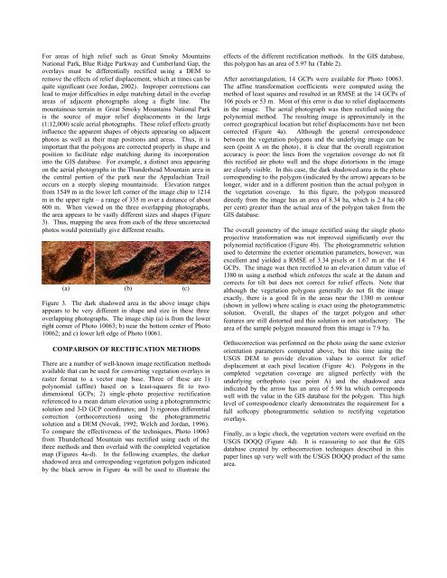
(a) (b) (c)<br />
Figure 3. The dark shadowed area in <strong>the</strong> above image chips<br />
appears to be very different in shape <strong>and</strong> size in <strong>the</strong>se three<br />
overlapping photographs. The image chip (a) is from <strong>the</strong> lower<br />
right corner of Photo 10063; b) near <strong>the</strong> bottom center of Photo<br />
10062; <strong>and</strong> c) lower left edge of Photo 10061.<br />
COMPARISON OF RECTIFICATION METHODS<br />
There are a number of well-known image rectification methods<br />
available that can be used for converting vegetation overlays in<br />
raster format to a vector map base. Three of <strong>the</strong>se are 1)<br />
polynomial (affine) based on a least-squares fit to twodimensional<br />
GCPs; 2) single -photo projective rectification<br />
referenced to a mean datum elevation using a photogrammetric<br />
solution <strong>and</strong> 3-D GCP coordinates; <strong>and</strong> 3) rigorous differential<br />
correction (orthocorrection) using <strong>the</strong> photogrammetric<br />
solution <strong>and</strong> a DEM (Novak, 1992; Welch <strong>and</strong> Jordan, 1996).<br />
To compare <strong>the</strong> effectiveness of <strong>the</strong> techniques, Photo 10063<br />
from Thunderhead Mountain was rectified using each of <strong>the</strong><br />
three methods <strong>and</strong> <strong>the</strong>n overlaid with <strong>the</strong> completed vegetation<br />
map (Figures 4a-d). In <strong>the</strong> following examples, <strong>the</strong> darker<br />
shadowed area <strong>and</strong> corresponding vegetation polygon indicated<br />
by <strong>the</strong> black arrow in Figure 4a will be used to illustrate <strong>the</strong><br />
effects of <strong>the</strong> different rectification methods. In <strong>the</strong> GIS database,<br />
this polygon has an area of 5.97 ha (Table 2).<br />
After aerotriangulation, 14 GCPs were available for Photo 10063.<br />
The affine transformation coefficients were computed using <strong>the</strong><br />
method of least squares <strong>and</strong> resulted in an RMSE at <strong>the</strong> 14 GCPs of<br />
106 pixels or 53 m. Most of this error is due to relief displacements<br />
in <strong>the</strong> image. The aerial photograph was <strong>the</strong>n rectified using <strong>the</strong><br />
polynomial method. The resulting image is approximately in <strong>the</strong><br />
correct geographical location but relief displacements have not been<br />
corrected (Figure 4a). Although <strong>the</strong> general correspondence<br />
between <strong>the</strong> vegetation polygons <strong>and</strong> <strong>the</strong> underlying image can be<br />
seen (point A on <strong>the</strong> photo) , it is clear that <strong>the</strong> overall registration<br />
accuracy is poor: <strong>the</strong> lines from <strong>the</strong> vegetation coverage do not fit<br />
this rectified air photo well <strong>and</strong> <strong>the</strong> shape distortions in <strong>the</strong> image<br />
are clearly visible. In this case, <strong>the</strong> dark shadowed area in <strong>the</strong> photo<br />
corresponding to <strong>the</strong> polygon (indicated by <strong>the</strong> arrow) appears to be<br />
longer, wider <strong>and</strong> in a different position than <strong>the</strong> actual polygon in<br />
<strong>the</strong> vegetation coverage. In this figure, <strong>the</strong> polygon measured<br />
directly from <strong>the</strong> image has an area of 8.34 ha, which is 2.4 ha (40<br />
per cent) greater than <strong>the</strong> actual area of <strong>the</strong> polygon taken from <strong>the</strong><br />
GIS database.<br />
The overall geometry of <strong>the</strong> image rectified using <strong>the</strong> single photo<br />
projective transformation was not improved significantly over <strong>the</strong><br />
polynomial rectification (Figure 4b). The photogrammetric solution<br />
used to determine <strong>the</strong> exterior orientation parameters, however, was<br />
excellent <strong>and</strong> yielded a RMSE of 3.34 pixels or 1.67 m at <strong>the</strong> 14<br />
GCPs. The image was <strong>the</strong>n rectified to an elevation datum value of<br />
1380 m using a method which enforces <strong>the</strong> scale at <strong>the</strong> datum <strong>and</strong><br />
corrects for tilt but does not correct for relief effects. Note that<br />
although <strong>the</strong> vegetation polygons generally do not fit <strong>the</strong> image<br />
exactly, <strong>the</strong>re is a good fit in <strong>the</strong> areas near <strong>the</strong> 1380 m contour<br />
(shown in yellow) where scaling is exact using <strong>the</strong> photogrammetric<br />
solution. Overall, <strong>the</strong> shapes of <strong>the</strong> target polygon <strong>and</strong> o<strong>the</strong>r<br />
features are still distorted <strong>and</strong> this solution is not satisfactory. The<br />
area of <strong>the</strong> sample polygon measured from this image is 7.9 ha.<br />
Orthocorrection was performed on <strong>the</strong> photo using <strong>the</strong> same exterior<br />
orientation parameters computed above, but this time using <strong>the</strong><br />
<strong>USGS</strong> DEM to provide elevation values to correct for relief<br />
displacement at each pixel location (Figure 4c). Polygons in <strong>the</strong><br />
completed vegetation coverage are aligned perfectly with <strong>the</strong><br />
underlying orthophoto (see point A) <strong>and</strong> <strong>the</strong> shadowed area<br />
indicated by <strong>the</strong> arrow has an area of 5.98 ha which corresponds<br />
well with <strong>the</strong> value in <strong>the</strong> GIS database for <strong>the</strong> polygon. This high<br />
level of correspondence clearly demonstrates <strong>the</strong> requirement for a<br />
full softcopy photogrammetric solution to rectifying vegetation<br />
overlays.<br />
Finally, as a logic check, <strong>the</strong> vegetation vectors were overlaid on <strong>the</strong><br />
<strong>USGS</strong> DOQQ (Figure 4d). It is reassuring to see that <strong>the</strong> GIS<br />
database created by orthocorrection techniques described in this<br />
paper lines up very well with <strong>the</strong> <strong>USGS</strong> DOQQ product of <strong>the</strong> same<br />
area.