Vegetation Classification and Mapping Project Report - the USGS

More documents

Recommendations

Info

Welch, R., M. Remillard and R. Doren, 1995. GIS database development for South Florida’s National Parks and Preserves. Photogrammetric Engineering and Remote Sensing, 61(11): 1371-1381. White, P. and J. Morse, 2000. The Science Plan for the All Taxa Biodiversity Inventory in Great Smoky Mountains National Park, North Carolina and Tennessee. Discover Life in America, Gatlinburg, Tennessee, http://www.discoverlife.org/sc/science_plan.html. Whittaker, R., 1956. Vegetation of the Great Smoky Mountains. Ecolological Monographs 26:1-80. 44
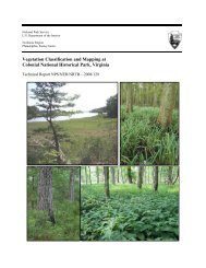
Control Extension and Orthorectification Procedures for Compiling Vegetation Databases of National Parks in the Southeastern United States Thomas R. Jordan Center for Remote Sensing and Mapping Science (CRMS) Department of Geography, The University of Georgia Athens, GA 30602 USA tombob@uga.edu Commission IV, WG IV/6 KEYWORDS: vegetation mapping; softcopy photogrammetry; GIS; mountainous terrain; national parks ABSTRACT: Vegetation mapping of national park units in the southeastern United States is being undertaken by the Center for Remote Sensing and Mapping Science at the University of Georgia. Because of the unique characteristics of the individual parks, including size, relief, number of photos and availability of ground control, different approaches are employed for converting vegetation polygons interpreted from large-scale color infrared aerial photographs and delineated on plastic overlays into accurately georeferenced GIS database layers. Using streamlined softcopy photogrammetry and aerotriangulation procedures, it is possible to differentially rectify overlays to compensate for relief displacements and create detailed vegetation maps that conform to defined mapping standards. This paper discusses the issues of ground control extension and orthorectification of photo overlays and describes the procedures employed in this project for building the vegetation GIS databases. INTRODUCTION The Center for Remote Sensing and Mapping Science (CRMS) at The University of Georgia has been engaged for several years in mapping vegetation communities in national parks in southeastern United States (Welch, et al., 2002). In this project, vegetation polygons delineated on overlays registered to large-scale (1:12,000 to 1:16,000 scale) color-infrared (CIR) aerial photographs are converted to digital format and integrated into a GIS database. To maximize vegetation discrimination, the aerial photographs are acquired during the autumn (leaf-on) season when the changing colors of the leaves provide additional indicators for species and vegetation community identification. It is critical that the polygons transferred from overlay to GIS database be accurate in terms of position, shape and size to ensure that analyses that depend on the interaction of layered data sets, such as fire fuel modelling and data visualization, can be performed with confidence (Madden, 2004). As many of these parks are located in remote and rugged areas where conventional sources of ground control are lacking, streamlined aerotriangulation procedures have been developed to extend the existing ground control and permit the production of orthophotos and corrected overlays for incorporation into the GIS database. STUDY AREA AND METHODOLOGY The overall project area encompasses much of the southeastern United States and includes U.S. National Park units located in the states of Kentucky, Tennessee, North Carolina, South Carolina, Virginia and Alabama (Figure 1). The parks differ greatly in size, location, relief and origin. Some of the smaller (100-400 ha) historical battlefield parks and national home sites in the project are located in or near urban areas with little relief and ample roads, field boundaries and other features that can be used for ground control. In these cases, ground control coordinates are extracted from U.S. Geological Survey (USGS) Digital Orthophoto Quarter Quadrangles (DOQQ) and simple polynomial techniques are applied to create corrected photos. Interpretation is then performed directly on the rectified CIR photographs and the polygons transferred into the GIS. rFODO Alabama STRI r rABLI MACA Tennessee LIRI -85 Kent ucky BISO OBRI Georgia CUGA GRSM West Virginia CARL r COWP r Virginia BLRI North Carolina NISI South Carolina r GUCO r 35 35 200 0 200 Kilometers -85 Figure 1. U.S. National Park units being mapped by the UGA- CRMS. See Table 1 below for park name abbreviations. Many of the parks, however, are set aside to protect natural areas ranging from 80 to over 2000 sq. km in size and require a large number of aerial photographs for complete coverage (Table 1). In the more remote areas, a recurring problem is the lack of cultural features suitable for use as the ground control required to restitute the aerial photographs and associated overlays. This issue is frequently exacerbated by the presence of extensive forest cover and high relief. The result is that the locations and shapes of vegetation polygons interpreted for -80 -80 N
Page 1 and 2: Digital Vegetation Maps for the Gre
Page 3 and 4: Table of Contents Page List of Figu
Page 5 and 6: List of Figures (Continued) Figure
Page 7 and 8: List of Attachments Attachment Atta
Page 9 and 10: and animals in the world. It has be
Page 11 and 12: logged or burned (Walker, 1991). Th
Page 13 and 14: The understory vegetation was mappe
Page 15 and 16: Photogrammetric Operations The main
Page 17 and 18: Figure 7. A mosaic of orthorectifie
Page 19 and 20: The term “overstory vegetation”
Page 21 and 22: provided in Attachment D, and furth
Page 23 and 24: Figure 11. Hardcopy vegetation maps
Page 25 and 26: to the terrain. Applications of the
Page 27 and 28: Figure 13. Total area (hectares) of
Page 29 and 30: Modeling Applications In addition t
Page 31 and 32: Fuel Class 1 Short Grass Fuel Class
Page 33 and 34: understory type and density, was th
Page 35 and 36: Figure 17. A sample of the fire fue
Page 37 and 38: The fuel class and percent canopy d
Page 39 and 40: interfaced to auxiliary data system
Page 41 and 42: References Albini, F. A., 1976. Est
Page 43: Moore, H.L.A., 1988. A Roadside Gui
Page 47 and 48: Figure 2. The vegetation map produc
Page 49 and 50: Table 2. Results of different image
Page 51 and 52: Attachment B Attachment B Vegetatio
Page 53 and 54: Attachment B Sub-Alpine Woodland 6.
Page 55 and 56: Attachment B c. S. Appalachian Cove
Page 57 and 58: Attachment B 10. White Oak-Red Mapl
Page 59 and 60: Attachment B E. Southern Blue Ridge
Page 61 and 62: Attachment B :G Graminoid spp. :Ht
Page 63 and 64: Attachment C Photointerpreters from
Page 65 and 66: Attachment C Our ecologically based
Page 67 and 68: Attachment C Mesic Oak-Hardwoods (l
Page 69 and 70: Attachment C Mixed (Virginia-Pitch-
Page 71 and 72: Attachment C prints for greatest di
Page 73 and 74: Attachment C the inhospitable smila
Page 75 and 76: Attachment C An NVCS association (a
Page 77 and 78: Attachment C only in protected cove
Page 79 and 80: Attachment C MOr/R-K (CEGL 7299) an
Page 81 and 82: Attachment C everything”: Fraser
Page 83 and 84: Attachment C 30. NHx:Bol, Southern
Page 85 and 86: Attachment C elevation, the hemlock
Page 87 and 88: Attachment C the surrounding tree c
Page 89 and 90: Attachment C Tom Govus should be al
Page 91 and 92: Attachment C Madden, M., 2003. Visu
Page 93 and 94: Attachment D species and it is beli
Page 95 and 96:
Attachment D Hemlock understory wit
Page 97 and 98:
Attachment D Spruce with heath bald
Page 99 and 100:
Attachment E Attachment E Notes on
Page 101 and 102:
Attachment E Springs, Wear Cove and
Page 103 and 104:
Attachment E number of leaves are n
Page 105 and 106:
Attachment F HxL 1403 4.9 0.0 141.1
Page 107 and 108:
Attachment F R/T 26 2.4 0.4 6.8 62.
Page 109 and 110:
Attachment G Attachment G Summary o
Page 111 and 112:
Attachment G PIsu/Rm 1 11.0 11.0 11
Page 113 and 114:
Attachment G T/PIs/Ri 53 6.6 0.7 31
Page 115 and 116:
Attachment H Vegetation Modeling, A
Page 117 and 118:
Attachment H Department of Agricult
Page 119 and 120:
Attachment H isolated from the over
Page 121:
Attachment H 8
show all

Vegetation Classification and Mapping Project Report - the USGS

You also want an ePaper? Increase the reach of your titles

Delete template?

Save as template?