Introduction to Microcontrollers

Introduction to Microcontrollers
Courses 182.064 & 182.074
Vienna University of Technology
Institute of Computer Engineering
Embedded Computing Systems Group
February 26, 2007
Version 1.4
Günther Gridling, Bettina Weiss

Contents
1 Microcontroller Basics 1
1.1 Introduction . . . . . . . . . . . . . . . . . . . . . . . . . . . . . . . . . . . . . . . 1
1.2 Frequently Used Terms . . . . . . . . . . . . . . . . . . . . . . . . . . . . . . . . . 6
1.3 Notation . . . . . . . . . . . . . . . . . . . . . . . . . . . . . . . . . . . . . . . . . 7
1.4 Exercises . . . . . . . . . . . . . . . . . . . . . . . . . . . . . . . . . . . . . . . . 8
2 Microcontroller Components 11
2.1 Processor Core . . . . . . . . . . . . . . . . . . . . . . . . . . . . . . . . . . . . . 11
2.1.1 Architecture . . . . . . . . . . . . . . . . . . . . . . . . . . . . . . . . . . . 11
2.1.2 Instruction Set . . . . . . . . . . . . . . . . . . . . . . . . . . . . . . . . . 15
2.1.3 Exercises . . . . . . . . . . . . . . . . . . . . . . . . . . . . . . . . . . . . 21
2.2 Memory . . . . . . . . . . . . . . . . . . . . . . . . . . . . . . . . . . . . . . . . . 22
2.2.1 Volatile Memory . . . . . . . . . . . . . . . . . . . . . . . . . . . . . . . . 23
2.2.2 Non-volatile Memory . . . . . . . . . . . . . . . . . . . . . . . . . . . . . . 27
2.2.3 Accessing Memory . . . . . . . . . . . . . . . . . . . . . . . . . . . . . . . 29
2.2.4 Exercises . . . . . . . . . . . . . . . . . . . . . . . . . . . . . . . . . . . . 31
2.3 Digital I/O . . . . . . . . . . . . . . . . . . . . . . . . . . . . . . . . . . . . . . . . 33
2.3.1 Digital Input . . . . . . . . . . . . . . . . . . . . . . . . . . . . . . . . . . 34
2.3.2 Digital Output . . . . . . . . . . . . . . . . . . . . . . . . . . . . . . . . . 38
2.3.3 Exercises . . . . . . . . . . . . . . . . . . . . . . . . . . . . . . . . . . . . 39
2.4 Analog I/O . . . . . . . . . . . . . . . . . . . . . . . . . . . . . . . . . . . . . . . 40
2.4.1 Digital/Analog Conversion . . . . . . . . . . . . . . . . . . . . . . . . . . . 40
2.4.2 Analog Comparator . . . . . . . . . . . . . . . . . . . . . . . . . . . . . . . 41
2.4.3 Analog/Digital Conversion . . . . . . . . . . . . . . . . . . . . . . . . . . . 42
2.4.4 Exercises . . . . . . . . . . . . . . . . . . . . . . . . . . . . . . . . . . . . 51
2.5 Interrupts . . . . . . . . . . . . . . . . . . . . . . . . . . . . . . . . . . . . . . . . 52
2.5.1 Interrupt Control . . . . . . . . . . . . . . . . . . . . . . . . . . . . . . . . 52
2.5.2 Interrupt Handling . . . . . . . . . . . . . . . . . . . . . . . . . . . . . . . 55
2.5.3 Interrupt Service Routine . . . . . . . . . . . . . . . . . . . . . . . . . . . . 57
2.5.4 Exercises . . . . . . . . . . . . . . . . . . . . . . . . . . . . . . . . . . . . 59
2.6 Timer . . . . . . . . . . . . . . . . . . . . . . . . . . . . . . . . . . . . . . . . . . 60
2.6.1 Counter . . . . . . . . . . . . . . . . . . . . . . . . . . . . . . . . . . . . . 60
2.6.2 Input Capture . . . . . . . . . . . . . . . . . . . . . . . . . . . . . . . . . . 62
2.6.3 Output Compare . . . . . . . . . . . . . . . . . . . . . . . . . . . . . . . . 65
2.6.4 Pulse Width Modulation . . . . . . . . . . . . . . . . . . . . . . . . . . . . 65
2.6.5 Exercises . . . . . . . . . . . . . . . . . . . . . . . . . . . . . . . . . . . . 66
2.7 Other Features . . . . . . . . . . . . . . . . . . . . . . . . . . . . . . . . . . . . . . 68
2.7.1 Watchdog Timer . . . . . . . . . . . . . . . . . . . . . . . . . . . . . . . . 68
i

2.7.2 Power Consumption and Sleep . . . . . . . . . . . . . . . . . . . . . . . . . 69
2.7.3 Reset . . . . . . . . . . . . . . . . . . . . . . . . . . . . . . . . . . . . . . 70
2.7.4 Exercises . . . . . . . . . . . . . . . . . . . . . . . . . . . . . . . . . . . . 71
3 Communication Interfaces 73
3.1 SCI (UART) . . . . . . . . . . . . . . . . . . . . . . . . . . . . . . . . . . . . . . . 75
3.2 SPI . . . . . . . . . . . . . . . . . . . . . . . . . . . . . . . . . . . . . . . . . . . . 82
3.3 IIC (I 2 C) . . . . . . . . . . . . . . . . . . . . . . . . . . . . . . . . . . . . . . . . 83
3.3.1 Data Transmission . . . . . . . . . . . . . . . . . . . . . . . . . . . . . . . 84
3.3.2 Speed Control Through Slave . . . . . . . . . . . . . . . . . . . . . . . . . 87
3.3.3 Multi-Master Mode . . . . . . . . . . . . . . . . . . . . . . . . . . . . . . . 87
3.3.4 Extended Addresses . . . . . . . . . . . . . . . . . . . . . . . . . . . . . . 88
3.4 Exercises . . . . . . . . . . . . . . . . . . . . . . . . . . . . . . . . . . . . . . . . 88
4 Software Development 89
4.1 Development Cycle . . . . . . . . . . . . . . . . . . . . . . . . . . . . . . . . . . . 91
4.1.1 Design Phase . . . . . . . . . . . . . . . . . . . . . . . . . . . . . . . . . . 91
4.1.2 Implementation . . . . . . . . . . . . . . . . . . . . . . . . . . . . . . . . . 92
4.1.3 Testing & Debugging . . . . . . . . . . . . . . . . . . . . . . . . . . . . . . 94
4.2 Programming . . . . . . . . . . . . . . . . . . . . . . . . . . . . . . . . . . . . . . 97
4.2.1 Assembly Language Programming . . . . . . . . . . . . . . . . . . . . . . . 97
4.3 Download . . . . . . . . . . . . . . . . . . . . . . . . . . . . . . . . . . . . . . . . 117
4.3.1 Programming Interfaces . . . . . . . . . . . . . . . . . . . . . . . . . . . . 117
4.3.2 Bootloader . . . . . . . . . . . . . . . . . . . . . . . . . . . . . . . . . . . 118
4.3.3 File Formats . . . . . . . . . . . . . . . . . . . . . . . . . . . . . . . . . . 118
4.4 Debugging . . . . . . . . . . . . . . . . . . . . . . . . . . . . . . . . . . . . . . . . 121
4.4.1 No Debugger . . . . . . . . . . . . . . . . . . . . . . . . . . . . . . . . . . 121
4.4.2 ROM Monitor . . . . . . . . . . . . . . . . . . . . . . . . . . . . . . . . . 124
4.4.3 Instruction Set Simulator . . . . . . . . . . . . . . . . . . . . . . . . . . . . 124
4.4.4 In-Circuit Emulator . . . . . . . . . . . . . . . . . . . . . . . . . . . . . . . 125
4.4.5 Debugging Interfaces . . . . . . . . . . . . . . . . . . . . . . . . . . . . . . 125
4.5 Exercises . . . . . . . . . . . . . . . . . . . . . . . . . . . . . . . . . . . . . . . . 127
5 Hardware 129
5.1 Switch/Button . . . . . . . . . . . . . . . . . . . . . . . . . . . . . . . . . . . . . . 129
5.2 Matrix Keypad . . . . . . . . . . . . . . . . . . . . . . . . . . . . . . . . . . . . . 130
5.3 Potentiometer . . . . . . . . . . . . . . . . . . . . . . . . . . . . . . . . . . . . . . 132
5.4 Phototransistor . . . . . . . . . . . . . . . . . . . . . . . . . . . . . . . . . . . . . 132
5.5 Position Encoder . . . . . . . . . . . . . . . . . . . . . . . . . . . . . . . . . . . . 133
5.6 LED . . . . . . . . . . . . . . . . . . . . . . . . . . . . . . . . . . . . . . . . . . . 134
5.7 Numeric Display . . . . . . . . . . . . . . . . . . . . . . . . . . . . . . . . . . . . 135
5.8 Multiplexed Display . . . . . . . . . . . . . . . . . . . . . . . . . . . . . . . . . . 136
5.9 Switching Loads . . . . . . . . . . . . . . . . . . . . . . . . . . . . . . . . . . . . 138
5.10 Motors . . . . . . . . . . . . . . . . . . . . . . . . . . . . . . . . . . . . . . . . . . 140
5.10.1 Basic Principles of Operation . . . . . . . . . . . . . . . . . . . . . . . . . 140
5.10.2 DC Motor . . . . . . . . . . . . . . . . . . . . . . . . . . . . . . . . . . . . 142
5.10.3 Stepper Motor . . . . . . . . . . . . . . . . . . . . . . . . . . . . . . . . . 146
5.11 Exercises . . . . . . . . . . . . . . . . . . . . . . . . . . . . . . . . . . . . . . . . 153
ii

A Table of Acronyms 155
Index 159
iii

Preface
This text has been developed for the introductory courses on microcontrollers taught by the Institute
of Computer Engineering at the Vienna University of Technology. It introduces undergraduate students
to the field of microcontrollers – what they are, how they work, how they interface with their
I/O components, and what considerations the programmer has to observe in hardware-based and embedded
programming. This text is not intended to teach one particular controller architecture in depth,
but should rather give an impression of the many possible architectures and solutions one can come
across in today’s microcontrollers. We concentrate, however, on small 8-bit controllers and their most
basic features, since they already offer enough variety to achieve our goals.
Since one of our courses is a lab and uses the ATmega16, we tend to use this Atmel microcontroller
in our examples. But we also use other controllers for demonstrations if appropriate.
For a few technical terms, we also give their German translations to allow our mainly Germanspeaking
students to learn both the English and the German term.
Please help us further improve this text by notifying us of errors. If you have any suggestions/wishes
like better and/or more thorough explanations, proposals for additional topics, . . . , feel
free to email us at mc-org@tilab.tuwien.ac.at.
v

Chapter 1
Microcontroller Basics
1.1 Introduction
Even at a time when Intel presented the first microprocessor with the 4004 there was alrady a demand
for microcontrollers: The contemporary TMS1802 from Texas Instruments, designed for usage in calculators,
was by the end of 1971 advertised for applications in cash registers, watches and measuring
instruments. The TMS 1000, which was introduced in 1974, already included RAM, ROM, and I/O
on-chip and can be seen as one of the first microcontrollers, even though it was called a microcomputer.
The first controllers to gain really widespread use were the Intel 8048, which was integrated
into PC keyboards, and its successor, the Intel 8051, as well as the 68HCxx series of microcontrollers
from Motorola.
Today, microcontroller production counts are in the billions per year, and the controllers are integrated
into many appliances we have grown used to, like
• household appliances (microwave, washing machine, coffee machine, . . . )
• telecommunication (mobile phones)
• automotive industry (fuel injection, ABS, . . . )
• aerospace industry
• industrial automation
• . . .
But what is this microcontroller we are talking about? What is the difference to a microprocessor?
And why do we need microcontrollers in the first place? To answer these questions, let us consider a
simple toy project: A heat control system. Assume that we want to
• periodically read the temperature (analog value, is digitized by sensor; uses 4-bit interface),
• control heating according to the temperature (turn heater on/off; 1 bit),
• display the current temperature on a simple 3-digit numeric display (8+3 bits),
• allow the user to adjust temperature thresholds (buttons; 4 bits), and
• be able to configure/upgrade the system over a serial interface.
So we design a printed-circuit board (PCB) using Zilog’s Z80 processor. On the board, we put a
Z80 CPU, 2 PIOs (parallel I/O; each chip has 16 I/O lines, we need 20), 1 SIO (serial I/O; for communication
to the PC), 1 CTC (Timer; for periodical actions), SRAM (for variables), Flash (for program
1

2 CHAPTER 1. MICROCONTROLLER BASICS
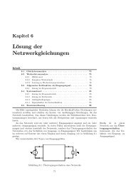
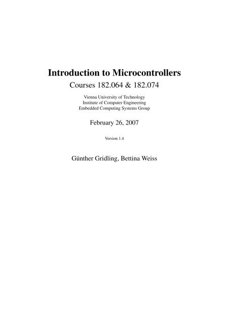
memory), and EEPROM (for constants). 1 The resulting board layout is depicted in Figure 1.1; as you
can see, there are a lot of chips on the board, which take up most of the space (euro format, 10 × 16
cm).
Figure 1.1: Z80 board layout for 32 I/O pins and Flash, EEPROM, SRAM.
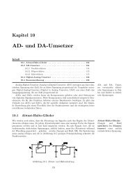
Incidentally, we could also solve the problem with the ATmega16 board we use in the Microcontroller
lab. In Figure 1.2, you can see the corresponding part of this board superposed on the Z80
PCB. The reduction in size is about a factor 5-6, and the ATmega16 board has even more features
than the Z80 board (for example an analog converter)! The reason why we do not need much space
for the ATmega16 board is that all those chips on the Z80 board are integrated into the ATmega16
microcontroller, resulting in a significant reduction in PCB size.
This example clearly demonstrates the difference between microcontroller and microprocessor: A
microcontroller is a processor with memory and a whole lot of other components integrated on one
chip. The example also illustrates why microcontrollers are useful: The reduction of PCB size saves
time, space, and money.
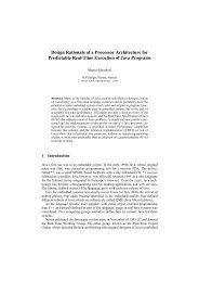
The difference between controllers and processors is also obvious from their pinouts. Figure 1.3
shows the pinout of the Z80 processor. You see a typical processor pinout, with address pins A0-
A15, data pins D0-D7, and some control pins like INT, NMI or HALT. In contrast, the ATmega16
has neither address nor data pins. Instead, it has 32 general purpose I/O pins PA0-PA7, PB0-PB7,
1 We also added a reset button and connectors for the SIO and PIO pins, but leave out the power supply circuitry and
the serial connector to avoid cluttering the layout.

1.1. INTRODUCTION 3
Figure 1.2: ATmega16 board superposed on the Z80 board.
Figure 1.3: Pinouts of the Z80 processor (left) and the ATmega16 controller (right).
PC0-PC7, PD0-PD7, which can be used for different functions. For example, PD0 and PD1 can be
used as the receive and transmit lines of the built-in serial interface. Apart from the power supply,
the only dedicated pins on the ATmega16 are RESET, external crystal/oscillator XTAL1 and XTAL2,
and analog voltage reference AREF.
Now that we have convinced you that microcontrollers are great, there is the question of which
microcontroller to use for a given application. Since costs are important, it is only logical to select
the cheapest device that matches the application’s needs. As a result, microcontrollers are generally
tailored for specific applications, and there is a wide variety of microcontrollers to choose from.
The first choice a designer has to make is the controller family – it defines the controller’s archi-

4 CHAPTER 1. MICROCONTROLLER BASICS
tecture. All controllers of a family contain the same processor core and hence are code-compatible,
but they differ in the additional components like the number of timers or the amount of memory.
There are numerous microcontrollers on the market today, as you can easily confirm by visiting the
webpages of one or two electronics vendors and browsing through their microcontroller stocks. You
will find that there are many different controller families like 8051, PIC, HC, ARM to name just a
few, and that even within a single controller family you may again have a choice of many different
controllers.
Controller Flash SRAM EEPROM I/O-Pins A/D Interfaces
(KB) (Byte) (Byte) (Channels)
AT90C8534 8 288 512 7 8
AT90LS2323 2 128 128 3
AT90LS2343 2 160 128 5
AT90LS8535 8 512 512 32 8 UART, SPI
AT90S1200 1 64 15
AT90S2313 2 160 128 15
ATmega128 128 4096 4096 53 8 JTAG, SPI, IIC
ATmega162 16 1024 512 35 JTAG, SPI
ATmega169 16 1024 512 53 8 JTAG, SPI, IIC
ATmega16 16 1024 512 32 8 JTAG, SPI, IIC
ATtiny11 1 64 5+1 In
ATtiny12 1 64 6 SPI
ATtiny15L 1 64 6 4 SPI
ATtiny26 2 128 128 16 SPI
ATtiny28L 2 128 11+8 In
Table 1.1: Comparison of AVR 8-bit controllers (AVR, ATmega, ATtiny).
Table 1.1 2 shows a selection of microcontrollers of Atmel’s AVR family. The one thing all these
controllers have in common is their AVR processor core, which contains 32 general purpose registers
and executes most instructions within one clock cycle.
After the controller family has been selected, the next step is to choose the right controller for
the job (see [Ber02] for a more in-depth discussion on selecting a controller). As you can see in
Table 1.1 (which only contains the most basic features of the controllers, namely memory, digital and
analog I/O, and interfaces), the controllers vastly differ in their memory configurations and I/O. The
chosen controller should of course cover the hardware requirements of the application, but it is also
important to estimate the application’s speed and memory requirements and to select a controller that
offers enough performance. For memory, there is a rule of thumb that states that an application should
take up no more than 80% of the controller’s memory – this gives you some buffer for later additions.
The rule can probably be extended to all controller resources in general; it always pays to have some
reserves in case of unforseen problems or additional features.
Of course, for complex applications a before-hand estimation is not easy. Furthermore, in 32bit
microcontrollers you generally also include an operating system to support the application and
2 This table was assembled in 2003. Even then, it was not complete; we have left out all controllers not recommended
for new designs, plus all variants of one type. Furthermore, we have left out several ATmega controllers. You can find a
complete and up-to-date list on the homepage of Atmel [Atm].

1.1. INTRODUCTION 5
its development, which increases the performance demands even more. For small 8-bit controllers,
however, only the application has to be considered. Here, rough estimations can be made for example
based on previous and/or similar projects.
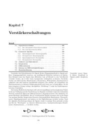
The basic internal designs of microcontrollers are pretty similar. Figure 1.4 shows the block
diagram of a typical microcontroller. All components are connected via an internal bus and are all
integrated on one chip. The modules are connected to the outside world via I/O pins.
Microcontroller
Processor
Core
Digital I/O
Module
...
SRAM
Serial
Interface
Module
Internal Bus
EEPROM/
Flash
Analog
Module
...
Counter/
Timer
Module
Interrupt
Controller
Figure 1.4: Basic layout of a microcontroller.
The following list contains the modules typically found in a microcontroller. You can find a more
detailed description of these components in later sections.
Processor Core: The CPU of the controller. It contains the arithmetic logic unit, the control unit,
and the registers (stack pointer, program counter, accumulator register, register file, . . . ).
Memory: The memory is sometimes split into program memory and data memory. In larger controllers,
a DMA controller handles data transfers between peripheral components and the memory.
Interrupt Controller: Interrupts are useful for interrupting the normal program flow in case of (important)
external or internal events. In conjunction with sleep modes, they help to conserve
power.
Timer/Counter: Most controllers have at least one and more likely 2-3 Timer/Counters, which can
be used to timestamp events, measure intervals, or count events.
Many controllers also contain PWM (pulse width modulation) outputs, which can be used to
drive motors or for safe breaking (antilock brake system, ABS). Furthermore the PWM output
can, in conjunction with an external filter, be used to realize a cheap digital/analog converter.
Digital I/O: Parallel digital I/O ports are one of the main features of microcontrollers. The number
of I/O pins varies from 3-4 to over 90, depending on the controller family and the controller
type.

6 CHAPTER 1. MICROCONTROLLER BASICS
Analog I/O: Apart from a few small controllers, most microcontrollers have integrated analog/digital
converters, which differ in the number of channels (2-16) and their resolution (8-12 bits). The
analog module also generally features an analog comparator. In some cases, the microcontroller
includes digital/analog converters.
Interfaces: Controllers generally have at least one serial interface which can be used to download the
program and for communication with the development PC in general. Since serial interfaces
can also be used to communicate with external peripheral devices, most controllers offer several
and varied interfaces like SPI and SCI.
Many microcontrollers also contain integrated bus controllers for the most common (field)busses.
IIC and CAN controllers lead the field here. Larger microcontrollers may also contain PCI,
USB, or Ethernet interfaces.
Watchdog Timer: Since safety-critical systems form a major application area of microcontrollers, it
is important to guard against errors in the program and/or the hardware. The watchdog timer is
used to reset the controller in case of software “crashes”.
Debugging Unit: Some controllers are equipped with additional hardware to allow remote debugging
of the chip from the PC. So there is no need to download special debugging software,
which has the distinct advantage that erroneous application code cannot overwrite the debugger.
Contrary to processors, (smaller) controllers do not contain a MMU (Memory Management Unit),
have no or a very simplified instruction pipeline, and have no cache memory, since both costs and
the ability to calculate execution times (some of the embedded systems employing controllers are
real-time systems, like X-by-wire systems in automotive control) are important issues in the microcontroller
market.
To summarize, a microcontroller is a (stripped-down) processor which is equipped with memory,
timers, (parallel) I/O pins and other on-chip peripherals. The driving element behind all this is cost:
Integrating all elements on one chip saves space and leads to both lower manufacturing costs and
shorter development times. This saves both time and money, which are key factors in embedded
systems. Additional advantages of the integration are easy upgradability, lower power consumption,
and higher reliability, which are also very important aspects in embedded systems. On the downside,
using a microcontroller to solve a task in software that could also be solved with a hardware solution
will not give you the same speed that the hardware solution could achieve. Hence, applications which
require very short reaction times might still call for a hardware solution. Most applications, however,
and in particular those that require some sort of human interaction (microwave, mobile phone), do not
need such fast reaction times, so for these applications microcontrollers are a good choice.
1.2 Frequently Used Terms
Before we concentrate on microcontrollers, let us first list a few terms you will frequently encounter
in the embedded systems field.
Microprocessor: This is a normal CPU (Central Processing Unit) as you can find in a PC. Communication
with external devices is achieved via a data bus, hence the chip mainly features data
and address pins as well as a couple of control pins. All peripheral devices (memory, floppy
controller, USB controller, timer, . . . ) are connected to the bus. A microprocessor cannot be

1.3. NOTATION 7
operated stand-alone, at the very least it requires some memory and an output device to be
useful.
Please note that a processor is no controller. Nevertheless, some manufacturers and vendors list
their controllers under the term “microprocessor”. In this text we use the term processor just
for the processor core (the CPU) of a microcontroller.
Microcontroller: A microcontroller already contains all components which allow it to operate standalone,
and it has been designed in particular for monitoring and/or control tasks. In consequence,
in addition to the processor it includes memory, various interface controllers, one or
more timers, an interrupt controller, and last but definitely not least general purpose I/O pins
which allow it to directly interface to its environment. Microcontrollers also include bit operations
which allow you to change one bit within a byte without touching the other bits.
Mixed-Signal Controller: This is a microcontroller which can process both digital and analog signals.
Embedded System: A major application area for microcontrollers are embedded systems. In embedded
systems, the control unit is integrated into the system 3 . As an example, think of a cell
phone, where the controller is included in the device. This is easily recognizable as an embedded
system. On the other hand, if you use a normal PC in a factory to control an assembly
line, this also meets many of the definitions of an embedded system. The same PC, however,
equipped with a normal operating system and used by the night guard to kill time is certainly
no embedded system.
Real-Time System: Controllers are frequently used in real-time systems, where the reaction to an
event has to occur within a specified time. This is true for many applications in aerospace,
railroad, or automotive areas, e.g., for brake-by-wire in cars.
Embedded Processor: This term often occurs in association with embedded systems, and the differences
to controllers are often very blurred. In general, the term “embedded processor” is used
for high-end devices (32 bits), whereas “controller” is traditionally used for low-end devices (4,
8, 16 bits). Motorola for example files its 32 bit controllers under the term “32-bit embedded
processors”.
Digital Signal Processor (DSP): Signal processors are used for applications that need to —no surprise
here— process signals. An important area of use are telecommunications, so your mobile
phone will probably contain a DSP. Such processors are designed for fast addition and multiplication,
which are the key operations for signal processing. Since tasks which call for a signal
processor may also include control functions, many vendors offer hybrid solutions which combine
a controller with a DSP on one chip, like Motorola’s DSP56800.
1.3 Notation
There are some notational conventions we will follow throughout the text. Most notations will be
explained anyway when they are first used, but here is a short overview:
3 The exact definition of what constitutes an embedded system is a matter of some dispute. Here is an example
definition of an online-encyclopaedia [Wik]:
An embedded system is a special-purpose computer system built into a larger device. An embedded system
is typically required to meet very different requirements than a general-purpose personal computer.
Other definitions allow the computer to be separate from the controlled device. All definitions have in common that the
computer/controller is designed and used for a special-purpose and cannot be used for general purpose tasks.

8 CHAPTER 1. MICROCONTROLLER BASICS
• When we talk about the values of digital lines, we generally mean their logical values, 0 or 1.
We indicate the complement of a logical value X with X, so 1 = 0 and 0 = 1.
• Hexadecimal values are denoted by a preceding $ or 0x. Binary values are either given like
decimal values if it is obvious that the value is binary, or they are marked with (·)2.
• The notation M[X] is used to indicate a memory access at address X.
• In our assembler examples, we tend to use general-purpose registers, which are labeled with R
and a number, e.g., R0.
• The ∝ sign means “proportional to”.
• In a few cases, we will need intervals. We use the standard interval notations, which are [.,.] for
a closed interval, [.,.) and (.,.] for half-open intervals, and (.,.) for an open interval. Variables
denoting intervals will be overlined, e.g. dlatch = (0, 1]. The notation dlatch+2 adds the constant
to the interval, resulting in (0, 1] + 2 = (2, 3].
• We use k as a generic variable, so do not be surprised if k means different things in different
sections or even in different paragraphs within a section.
Furthermore, you should be familiar with the following power prefixes 4 :
1.4 Exercises
Name Prefix Power Name Prefix Power
kilo k 10 3 milli m 10 −3
mega M 10 6 micro µ, u 10 −6
giga G 10 9 nano n 10 −9
tera T 10 12 pico p 10 −12
peta P 10 15 femto f 10 −15
exa E 10 18 atto a 10 −18
zetta Z 10 21 zepto z 10 −21
yotta Y 10 24 yocto y 10 −24
Table 1.2: Power Prefixes
Exercise 1.1 What is the difference between a microcontroller and a microprocessor?
Exercise 1.2 Why do microcontrollers exist at all? Why not just use a normal processor and add all
necessary peripherals externally?
Exercise 1.3 What do you believe are the three biggest fields of application for microcontrollers?
Discuss you answers with other students.
Exercise 1.4 Visit the homepage of some electronics vendors and compare their stock of microcontrollers.
(a) Do all vendors offer the same controller families and manufacturers?
often.
4 We include the prefixes for ±15 and beyond for completeness’ sake – you will probably not encounter them very

1.4. EXERCISES 9
(b) Are prices for a particular controller the same? If no, are the price differences significant?
(c) Which controller families do you see most often?
Exercise 1.5 Name the basic components of a microcontroller. For each component, give an example
where it would be useful.
Exercise 1.6 What is an embedded system? What is a real-time system? Are these terms synonyms?
Is one a subset of the other? Why or why not?
Exercise 1.7 Why are there so many microcontrollers? Wouldn’t it be easier for both manufacturers
and consumers to have just a few types?
Exercise 1.8 Assume that you have a task that requires 18 inputs, 15 outputs, and 2 analog inputs.
You also need 512 bytes to store data. Which controllers of Table 1.1 can you use for the application?

10 CHAPTER 1. MICROCONTROLLER BASICS

Chapter 2
Microcontroller Components
2.1 Processor Core
The processor core (CPU) is the main part of any microcontroller. It is often taken from an existing
processor, e.g. the MC68306 microcontroller from Motorola contains a 68000 CPU. You should already
be familiar with the material in this section from other courses, so we will briefly repeat the
most important things but will not go into details. An informative book about computer architecture
is [HP90] or one of its successors.
2.1.1 Architecture
to/from
Program
Memory
to/from
Data
Memory
CPU
dst
PC
Instruction Register
Control
Unit
R0 src2
R1
R2
R3
Register
File
SP
src1
OP
Status(CC) Reg
Z N O C
Flags
ALU
Result
Figure 2.1: Basic CPU architecture.
Data path
A basic CPU architecture is depicted in Figure 2.1. It consists of the data path, which executes
instructions, and of the control unit, which basically tells the data path what to do.
11

12 CHAPTER 2. MICROCONTROLLER COMPONENTS
Arithmetic Logic Unit
At the core of the CPU is the arithmetic logic unit (ALU), which is used to perform computations
(AND, ADD, INC, . . . ). Several control lines select which operation the ALU should perform on the
input data. The ALU takes two inputs and returns the result of the operation as its output. Source and
destination are taken from registers or from memory. In addition, the ALU stores some information
about the nature of the result in the status register (also called condition code register):
Z (Zero): The result of the operation is zero.
N (Negative): The result of the operation is negative, that is, the most significant bit (msb) of the
result is set (1).
O (Overflow): The operation produced an overflow, that is, there was a change of sign in a two’scomplement
operation.
C (Carry): The operation produced a carry.
Two’s complement
Since computers only use 0 and 1 to represent numbers, the question arose how to represent
negative integer numbers. The basic idea here is to invert all bits of a positive integer to get the
corresponding negative integer (this would be the one’s complement). But this method has the
slight drawback that zero is represented twice (all bits 0 and all bits 1). Therefore, a better way
is to represent negative numbers by inverting the positive number and adding 1. For +1 and a
4-bit representation, this leads to:
For zero, we obtain
1 = 0001 → −1 = 1110 + 1 = 1111.
0 = 0000 → −0 = 1111 + 1 = 0000,
so there is only one representation for zero now. This method of representation is called the
two’s complement and is used in microcontrollers. With n bits it represents values within
[−2 n−1 , 2 n−1 − 1].
Register File
The register file contains the working registers of the CPU. It may either consist of a set of general
purpose registers (generally 16–32, but there can also be more), each of which can be the source or
destination of an operation, or it consists of some dedicated registers. Dedicated registers are e.g.
an accumulator, which is used for arithmetic/logic operations, or an index register, which is used for
some addressing modes.
In any case, the CPU can take the operands for the ALU from the file, and it can store the operation’s
result back to the register file. Alternatively, operands/result can come from/be stored to the
memory. However, memory access is much slower than access to the register file, so it is usually wise
to use the register file if possible.

2.1. PROCESSOR CORE 13
Example: Use of Status Register
The status register is very useful for a number of things, e.g., for adding or subtracting numbers
that exceed the CPU word length. The CPU offers operations which make use of the carry flag,
like ADDC a (add with carry). Consider for example the operation 0x01f0 + 0x0220 on an 8-bit
CPU b c :
CLC ; clear carry flag
LD R0, #0xf0 ; load first low byte into register R0
ADDC R0, #0x20 ; add 2nd low byte with carry (carry

14 CHAPTER 2. MICROCONTROLLER COMPONENTS
0x01 SP 0x01
$FF
$FF
0x02 SP 0x02
0x01 0x01
$FF $FF
SP 0x02
0x01
$FF
SP
0x02
0x01
$FF
Push 0x01
SP
Push 0x02
SP
Pop R2
R0
0x02
Figure 2.2: Stack operation (write first).
to the last address in memory (if a push stores first and decrements afterwards) or to the last address
+ 1 (if the push decrements first).
As we have mentioned, the controller uses the stack during subroutine calls and interrupts, that is,
whenever the normal program flow is interrupted and should resume later on. Since the return address
is a pre-requisite for resuming program execution after the point of interruption, every controller
pushes at least the return address onto the stack. Some controllers even save register contents on the
stack to ensure that they do not get overwritten by the interrupting code. This is mainly done by
controllers which only have a small set of dedicated registers.
Control Unit
Apart from some special situations like a HALT instruction or the reset, the CPU constantly executes
program instructions. It is the task of the control unit to determine which operation should be executed
next and to configure the data path accordingly. To do so, another special register, the program
counter (PC), is used to store the address of the next program instruction. The control unit loads
this instruction into the instruction register (IR), decodes the instruction, and sets up the data path
to execute it. Data path configuration includes providing the appropriate inputs for the ALU (from
registers or memory), selecting the right ALU operation, and making sure that the result is written
to the correct destination (register or memory). The PC is either incremented to point to the next
instruction in the sequence, or is loaded with a new address in the case of a jump or subroutine call.
After a reset, the PC is typically initialized to $0000.
Traditionally, the control unit was hard-wired, that is, it basically contained a look-up table which
held the values of the control lines necessary to perform the instruction, plus a rather complex decoding
logic. This meant that it was difficult to change or extend the instruction set of the CPU. To
ease the design of the control unit, Maurice Wilkes reflected that the control unit is actually a small
CPU by itself and could benefit from its own set of microinstructions. In his subsequent control unit
design, program instructions were broken down into microinstructions, each of which did some small
part of the whole instruction (like providing the correct register for the ALU). This essentially made
control design a programming task: Adding a new instruction to the instruction set boiled down to
programming the instruction in microcode. As a consequence, it suddenly became comparatively

2.1. PROCESSOR CORE 15
easy to add new and complex instructions, and instruction sets grew rather large and powerful as a
result. This earned the architecture the name Complex Instruction Set Computer (CISC). Of course,
the powerful instruction set has its price, and this price is speed: Microcoded instructions execute
slower than hard-wired ones. Furthermore, studies revealed that only 20% of the instructions of a
CISC machine are responsible for 80% of the code (80/20 rule). This and the fact that these complex
instructions can be implemented by a combination of simple ones gave rise to a movement back
towards simple hard-wired architectures, which were correspondingly called Reduced Instruction Set
Computer (RISC).
RISC: The RISC architecture has simple, hard-wired instructions which often take only one or a few
clock cycles to execute. RISC machines feature a small and fixed code size with comparatively
few instructions and few addressing modes. As a result, execution of instructions is very fast,
but the instruction set is rather simple.
CISC: The CISC architecture is characterized by its complex microcoded instructions which take
many clock cycles to execute. The architecture often has a large and variable code size and
offers many powerful instructions and addressing modes. In comparison to RISC, CISC takes
longer to execute its instructions, but the instruction set is more powerful.
Of course, when you have two architectures, the question arises which one is better. In the case
of RISC vs. CISC, the answer depends on what you need. If your solution frequently employs a
powerful instruction or addressing mode of a given CISC architecture, you probably will be better off
using CISC. If you mainly need simple instructions and addressing modes, you are most likely better
off using RISC. Of course, this choice also depends on other factors like the clocking frequencies of
the processors in question. In any case, you must know what you require from the architecture to
make the right choice.
Von Neumann versus Harvard Architecture
In Figure 2.1, instruction memory and data memory are depicted as two separate entities. This is
not always the case, both instructions and data may well be in one shared memory. In fact, whether
program and data memory are integrated or separate is the distinction between two basic types of
architecture:
Von Neumann Architecture: In this architecture, program and data are stored together and are accessed
through the same bus. Unfortunately, this implies that program and data accesses may
conflict (resulting in the famous von Neumann bottleneck), leading to unwelcome delays.
Harvard Architecture: This architecture demands that program and data are in separate memories
which are accessed via separate buses. In consequence, code accesses do not conflict with data
accesses which improves system performance. As a slight drawback, this architecture requires
more hardware, since it needs two busses and either two memory chips or a dual-ported memory
(a memory chip which allows two independent accesses at the same time).
2.1.2 Instruction Set
The instruction set is an important characteristic of any CPU. It influences the code size, that is, how
much memory space your program takes. Hence, you should choose the controller whose instruction
set best fits your specific needs. The metrics of the instruction set that are important for a design
decision are

16 CHAPTER 2. MICROCONTROLLER COMPONENTS
Example: CISC vs. RISC
Let us compare a complex CISC addressing mode with its implementation in a RISC architecture.
The 68030 CPU from Motorola offers the addressing mode “memory indirect preindexed,
scaled”:
MOVE D1, ([24,A0,4*D0])
This operation stores the contents of register D1 into the memory address
24 + [A0] + 4 ∗ [D0]
where square brackets designate “contents of” the register or memory address.
To simulate this addressing mode on an Atmel-like RISC CPU, we need something like the
following:
LD R1, X ; load data indirect (from [X] into R1)
LSL R1 ; shift left -> multiply with 2
LSL R1 ; 4*[D0] completed
MOV X, R0 ; set pointer (load A0)
LD R0, X ; load indirect ([A0] completed)
ADD R0, R1 ; add obtained pointers ([A0]+4*[D0])
LDI R1, $24 ; load constant ($ = hex)
ADD R0, R1 ; and add (24+[A0]+4*[D0])
MOV X, R0 ; set up pointer for store operation
ST X, R2 ; write value ([24+[A0]+4*[D0]]

2.1. PROCESSOR CORE 17
Example: Some opcodes of the ATmega16
The ATmega16 is an 8-bit harvard RISC controller with a fixed opcode size of 16 or in some
cases 32 bits. The controller has 32 general purpose registers. Here are some of its instructions
with their corresponding opcodes.
instruction result operand conditions opcode
ADD Rd, Rr Rd + Rd ← Rr 0 ≤ d ≤ 31, 0000 11rd dddd rrrr
0 ≤ r ≤ 31
AND Rd, Rr Rd ← Rd & Rr 0 ≤ d ≤ 31, 0010 00rd dddd rrrr
0 ≤ r ≤ 31
NOP 0000 0000 0000 0000
LDI Rd, K Rd ← K 16 ≤ d ≤ 31, 1110 KKKK dddd KKKK
0 ≤ K ≤ 255
LDS Rd, k Rd ← [k] 0 ≤ d ≤ 31, 1001 000d dddd 0000
0 ≤ k ≤ 65535 kkkk kkkk kkkk kkkk
Note that the LDI instruction, which loads a register with a constant, only operates on the upper
16 out of the whole 32 registers. This is necessary because there is no room in the 16 bit to
store the 5th bit required to address the lower 16 registers as well, and extending the operation
to 32 bits just to accommodate one more bit would be an exorbitant waste of resources.
The last instruction, LDS, which loads data from the data memory, actually requires 32 bits
to accommodate the memory address, so the controller has to perform two program memory
accesses to load the whole instruction.
what you need. For instance, the 10 lines of ATmega16 RISC code require 20 byte of code (each
instruction is encoded in 16 bits), whereas the 68030 instruction fits into 4 bytes. So here, the 68030
clearly wins. If, however, you only need instructions already provided by an architecture with short
opcodes, it will most likely beat a machine with longer opcodes. We say “most likely” here, because
CISC machines with long opcodes tend to make up for this deficit with variable size instructions. The
idea here is that although a complex operation with many operands may require 32 bits to encode,
a simple NOP (no operation) without any arguments could fit into 8 bits. As long as the first byte
of an instructions makes it clear whether further bytes should be decoded or not, there is no reason
not to allow simple instructions to take up only one byte. Of course, this technique makes instruction
fetching and decoding more complicated, but it still beats the overhead of a large fixed-size opcode.
RISC machines, on the other hand, tend to feature short but fixed-size opcodes to simplify instruction
decoding.
Obviously, a lot of space in the opcode is taken up by the operands. So one way of reducing the
instruction size is to cut back on the number of operands that are explicitly encoded in the opcode.
In consequence, we can distinguish four different architectures, depending on how many explicit
operands a binary operation like ADD requires:
Stack Architecture: This architecture, also called 0-address format architecture, does not have any
explicit operands. Instead, the operands are organized as a stack: An instruction like ADD takes
the top-most two values from the stack, adds them, and puts the result on the stack.
Accumulator Architecture: This architecture, also called 1-address format architecture, has an ac-

18 CHAPTER 2. MICROCONTROLLER COMPONENTS
cumulator which is always used as one of the operands and as the destination register. The
second operand is specified explicitly.
2-address Format Architecture: Here, both operands are specified, but one of them is also used
as the destination to store the result. Which register is used for this purpose depends on the
processor in question, for example, the ATmega16 controller uses the first register as implicit
destination, whereas the 68000 processor uses the second register.
3-address Format Architecture: In this architecture, both source operands and the destination are
explicitly specified. This architecture is the most flexible, but of course it also has the longest
instruction size.
Table 2.1 shows the differences between the architectures when computing (A+B)*C. We assume
that in the cases of the 2- and 3-address format, the result is stored in the first register. We also
assume that the 2- and 3-address format architectures are load/store architectures, where arithmetic
instructions only operate on registers. The last line in the table indicates where the result is stored.
Execution Speed
stack accumulator 2-address format 3-address format
PUSH A LOAD A LOAD R1, A LOAD R1, A
PUSH B ADD B LOAD R2, B LOAD R2, B
ADD MUL C ADD R1, R2 ADD R1, R1, R2
PUSH C LOAD R2, C LOAD R2, C
MUL MUL R1, R2 MUL R1, R1, R2
stack accumulator R1 R1
Table 2.1: Comparison between architectures.
The execution speed of an instruction depends on several factors. It is mostly influenced by the
complexity of the architecture, so you can generally expect a CISC machine to require more cycles to
execute an instruction than a RISC machine. It also depends on the word size of the machine, since a
machine that can fetch a 32 bit instruction in one go is faster than an 8-bit machine that takes 4 cycles
to fetch such a long instruction. Finally, the oscillator frequency defines the absolute speed of the
execution, since a CPU that can be operated at 20 MHz can afford to take twice as many cycles and
will still be faster than a CPU with a maximum operating frequency of 8 MHz.
Available Instructions
Of course, the nature of available instructions is an important criterion for selecting a controller.
Instructions are typically parted into several classes:
Arithmetic-Logic Instructions: This class contains all operations which compute something, e.g.,
ADD, SUB, MUL, . . . , and logic operations like AND, OR, XOR, . . . . It may also contain bit
operations like BSET (set a bit), BCLR (clear a bit), and BTST (test whether a bit is set). Bit
operations are an important feature of the microcontroller, since it allows to access single bits
without changing the other bits in the byte. As we will see in Section 2.3, this is a very useful
feature to have.

2.1. PROCESSOR CORE 19
Shift operations, which move the contents of a register one bit to the left or to the right, are
typically provided both as logical and as arithmetical operations. The difference lies in their
treatment of the most significant bit when shifting to the right (which corresponds to a division
by 2). Seen arithmetically, the msb is the sign bit and should be kept when shifting to the right.
So if the msb is set, then an arithmetic right-shift will keep the msb set. Seen logically, however,
the msb is like any other bit, so here a right-shift will clear the msb. Note that there is no need
to keep the msb when shifting to the left (which corresponds to a multiplication by 2). Here, a
simple logical shift will keep the msb set anyway as long as there is no overflow. If an overflow
occurs, then by not keeping the msb we simply allow the result to wrap, and the status register
will indicate that the result has overflowed. Hence, an arithmetic shift to the left is the same as
a logical shift.
Example: Arithmetic shift
To illustrate what happens in an arithmetic shift to the left, consider a 4-bit machine.
Negative numbers are represented in two’s complement, so for example -7 is represented
as binary 1001. If we simply shift to the left, we obtain 0010 = 2, which is the same as
-14 modulo 16. If we had kept the msb, the result would have been 1010 = -6, which is
simply wrong.
Shifting to the right can be interpreted as a division by two. If we arithmetically right-shift
-4 = 1100, we obtain 1110 = -2 since the msb remains set. In a logical shift to the right,
the result would have been 0110 = 6.
Data Transfer: These operations transfer data between two registers, between registers and memory,
or between memory locations. They contain the normal memory access instructions like LD
(load) and ST (store), but also the stack access operations PUSH and POP.
Program Flow: Here you will find all instructions which influence the program flow. These include
jump instructions which set the program counter to a new address, conditional branches like
BNE (branch if the result of the prior instruction was not zero), subroutine calls, and calls that
return from subroutines like RET or RETI (return from interrupt service routine).
Control Instructions: This class contains all instructions which influence the operation of the controller.
The simplest such instruction is NOP, which tells the CPU to do nothing. All other
special instructions, like power-management, reset, debug mode control, . . . also fall into this
class.
Addressing Modes
When using an arithmetic instruction, the application programmer must be able to specify the instruction’s
explicit operands. Operands may be constants, the contents of registers, or the contents
of memory locations. Hence, the processor has to provide means to specify the type of the operand.
While every processor allows you to specify the above-mentioned types, access to memory locations
can be done in many different ways depending on what is required. So the number and types of
addressing modes provided is another important characteristic of any processor. There are numerous
addressing modes 2 , but we will restrict ourselves to the most common ones.
2 Unfortunately, there is no consensus about the names of the addressing modes. We follow [HP90, p. 98] in our
nomenclature, but you may also find other names for these addressing modes in the literature.

20 CHAPTER 2. MICROCONTROLLER COMPONENTS
immediate/literal: Here, the operand is a constant. From the application programmer’s point of
view, processors may either provide a distinct instruction for constants (like the LDI —load
immediate— instruction of the ATmega16), or require the programmer to flag constants in the
assembler code with some prefix like #.
register: Here, the operand is the register that contains the value or that should be used to store the
result.
direct/absolute: The operand is a memory location.
register indirect: Here, a register is specified, but it only contains the memory address of the actual
source or destination. The actual access is to this memory location.
autoincrement: This is a variant of indirect addressing where the contents of the specified register is
incremented either before (pre-increment) or after (post-increment) the access to the memory
location. The post-increment variant is very useful for iterating through an array, since you
can store the base address of the array as an index into the array and then simply access each
element in one instruction, while the index gets incremented automatically.
autodecrement: This is the counter-part to the autoincrement mode, the register value gets decremented
either before or after the access to the memory location. Again nice to have when
iterating through arrays.
displacement/based: In this mode, the programmer specifies a constant and a register. The contents
of the register is added to the constant to get the final memory location. This can again be used
for arrays if the constant is interpreted as the base address and the register as the index within
the array.
indexed: Here, two registers are specified, and their contents are added to form the memory address.
The mode is similar to the displacement mode and can again be used for arrays by storing the
base address in one register and the index in the other. Some controllers use a special register
as the index register. In this case, it does not have to be specified explicitly.
memory indirect: The programmer again specifies a register, but the corresponding memory location
is interpreted as a pointer, i.e., it contains the final memory location. This mode is quite
useful, for example for jump tables.
Table 2.2 shows the addressing modes in action. In the table, M[x] is an access to the memory
address x, d is the data size, and #n indicates a constant. The notation is taken from [HP90] and
varies from controller to controller.
As we have already mentioned, CISC processors feature more addressing modes than RISC processors,
so RISC processors must construct more complex addressing modes with several instructions.
Hence, if you often need a complex addressing mode, a CISC machine providing this mode may be
the wiser choice.
Before we close this section, we would like to introduce you to a few terms you will often encounter:
• An instruction set is called orthogonal if you can use every instruction with every addressing
mode.
• If it is only possible to address memory with special memory access instructions (LOAD,
STORE), and all other instructions like arithmetic instructions only operate on registers, the
architecture is called a load/store architecture.
• If all registers have the same function (apart from a couple of system registers like the PC or
the SP), then these registers are called general-purpose registers.

2.1. PROCESSOR CORE 21
2.1.3 Exercises
addressing mode example result
immediate ADD R1, #5 R1 ← R1 + 5
register ADD R1, R2 R1 ← R1 + R2
direct ADD R1, 100 R1 ← R1 + M[100]
register indirect ADD R1, (R2) R1 ← R1 + M[R2]
post-increment ADD R1, (R2)+ R1 ← R1 + M[R2]
R2 ← R2 + d
pre-decrement ADD R1, −(R2) R2 ← R2 − d
R1 ← R1 + M[R2]
displacement ADD R1, 100(R2) R1 ← R1 + M[100 + R2]
indexed ADD R1, (R2+R3) R1 ← R1 + M[R2+R3]
memory indirect ADD R1, @(R2) R1 ← R1 + M[M[R2]]
Table 2.2: Comparison of addressing modes.
Exercise 2.1.1 What are the advantages of the Harvard architecture in relation to the von Neumann
architecture? If you equip a von Neumann machine with a dual-ported RAM (that is a RAM which
allows two concurrent accesses), does this make it a Harvard machine, or is there still something
missing?
Exercise 2.1.2 Why was RISC developed? Why can it be faster to do something with several instructions
instead of just one?
Exercise 2.1.3 What are the advantages of general-purpose registers as opposed to dedicated registers?
What are their disadvantages?
Exercise 2.1.4 In Section 2.1.2, we compared different address formats. In our example, the accumulator
architecture requires the least instructions to execute the task. Does this mean that accumulator
architectures are particularly code-efficient?
Exercise 2.1.5 What are the advantages and drawbacks of a load/store architecture?
Exercise 2.1.6 Assume that you want to access an array consisting of 10 words (a word has 16 bit)
starting at memory address 100. Write an assembler program that iterates through the array (pseudocode).
Compare the addressing modes register indirect, displacement, auto-increment, and indexed.
Exercise 2.1.7 Why do negative numbers in an arithmetic shift left (ASL) stay negative as long as
there is no overflow, even though the sign bit is not treated any special? Can you prove that the sign
bit remains set in an ASL as long as there is no overflow? Is it always true that even with an overflow
the result will remain correct (modulo the range)?

22 CHAPTER 2. MICROCONTROLLER COMPONENTS
2.2 Memory
In the previous chapter, you already encountered various memory types: The register file is, of course,
just a small memory embedded in the CPU. Also, we briefly mentioned data being transferred between
registers and the data memory, and instructions being fetched from the instruction memory.
Therefore, an obvious distinction of memory types can be made according to their function:
Register File: A (usually) relatively small memory embedded on the CPU. It is used as a scratchpad
for temporary storage of values the CPU is working with - you could call it the CPU’s short
term memory.
Data Memory: For longer term storage, generic CPUs usually employ an external memory which is
much larger than the register file. Data that is stored there may be short-lived, but may also be
valid for as long as the CPU is running. Of course, attaching external memory to a CPU requires
some hardware effort and thus incurs some cost. For that reason, microcontrollers usually sport
on-chip data memory.
Instruction Memory: Like the data memory, the instruction memory is usually a relatively large
external memory (at least with general CPUs). Actually, with von-Neumann-architectures,
it may even be the same physical memory as the data memory. With microcontrollers, the
instruction memory, too, is usually integrated right into the MCU.
These are the most prominent uses of memory in or around a CPU. However, there is more memory
in a CPU than is immediately obvious. Depending on the type of CPU, there can be pipeline
registers, caches, various buffers, and so on.
About memory embedded in an MCU: Naturally, the size of such on-chip memory is limited. Even
worse, it is often not possible to expand the memory externally (in order to keep the design simple).
However, since MCUs most often are used for relatively simple tasks and hence do not need excessive
amounts of memory, it is prudent to include a small amount of data and instruction memory on the
chip. That way, total system cost is decreased considerably, and even if the memory is not expandable,
you are not necessarily stuck with it: Different members in a MCU family usually provide different
amounts of memory, so you can choose a particular MCU which offers the appropriate memory space.
Now, the functional distinction of memory types made above is based on the way the memory is
used. From a programmer’s perspective, that makes sense. However, hardware or chip designers usually
view memory rather differently: They prefer to distinguish according to the physical properties
of the electronic parts the memory is made of. There, the most basic distinction would be volatile
versus non-volatile memory. In this context, volatile means that the contents of the memory are lost
as soon as the system’s power is switched off.
Of course, there are different ways either type of memory can be implemented. Therefore, the
distinction based on the physical properties can go into more detail. Volatile memory can be static or
dynamic, and there is quite a variety of non-volatile memory types: ROM, PROM, EPROM, EEPROM,
FLASH, NV-RAM. Let’s examine those more closely.

2.2. MEMORY 23
SRAM DRAM
Semiconductor
Memory
volatile non−volatile
2.2.1 Volatile Memory
ROM PROM EPROM EEPROM
Figure 2.3: Types of Semiconductor Memory.
Flash
EEPROM
NVRAM
As mentioned above, volatile memory retains its contents only so long as the system is powered on.
Then why should you use volatile memory at all, when non-volatile memory is readily available?
The problem here is that non-volatile memory is usually a lot slower, more involved to work with,
and much more expensive. While the volatile memory in your PC has access times in the nanosecond
range, some types of non-volatile memory will be unavailable for milliseconds after writing one lousy
byte to them.
Where does the name RAM come from?
For historic reasons, volatile memory is generally called RAM – Random Access Memory.
Of course, the random part does not mean that chance is involved in accessing the memory.
That acronym was coined at an early stage in the development of computers. Back then,
there were different types of volatile memory: One which allowed direct access to any
address, and one which could only be read and written sequentially (so-called shift register
memory). Engineers decided to call the former type ‘random access memory’, to reflect
the fact that, from the memory’s perspective, any ‘random’, i.e., arbitrary, address could
be accessed. The latter type of memory is not commonly used any more, but the term
RAM remains.
Static RAM
Disregarding the era of computers before the use of integrated circuits, Static Random Access Memory
(SRAM) was the first type of volatile memory to be widely used. An SRAM chip consists of an array
of cells, each capable of storing one bit of information. To store a bit of information, a so-called
flip-flop is used, which basically consists of six transistors. For now, the internal structure of such a
cell is beyond the scope of our course, so let’s just view the cell as a black box. Looking at Figure 2.4,
you see that one SRAM cell has the following inputs and outputs:
Data In Din On this input, the cell accepts the one bit of data to be stored.
Data Out Dout As the name implies, this output reflects the bit that is stored in the cell.

24 CHAPTER 2. MICROCONTROLLER COMPONENTS
Read/Write R/W Via the logical value at this input, the type of access is specified: 0 means the cell
is to be written to, i.e., the current state of Din should be stored in the cell. 1 means that the cell
is to be read, so it should set Dout to the stored value.
Cell Select CS As long as this input is logical 0, the cell does not accept any data present at Din and
keeps its output Dout in a so-called high resistance state, which effectively disconnects it from
the rest of the system. On a rising edge, the cell either accepts the state at Din as the new bit to
store, or it sets Dout to the currently stored value.
Din
R/W
CS
SRAM
Memory
Cell
D out
Figure 2.4: An SRAM cell as a black box.
To get a useful memory, many such cells are arranged in a matrix as depicted in Figure 2.5. As
you can see, all Dout lines are tied together. If all cells would drive their outputs despite not being
addressed, a short between GND and VCC might occur, which would most likely destroy the chip.
Therefore, the CS line is used to select one cell in the matrix and to put all other cells into their high
resistance state. To address one cell and hence access one particular bit, SRAMs need some extra
logic to facilitate such addressing (note that we use, of course, a simplified diagram).
row0
row1
row2
row3
&
&
&
&
SRAM Cell
D in
R/W
CS
D in
R/W
CS
D out
SRAM Cell
D in
R/W
CS
D out
SRAM Cell
D Dout out
SRAM Cell
D in
R/W
CS
D out
&
&
&
&
SRAM Cell
D in
R/W
CS
D in
R/W
CS
D out
SRAM Cell
D in
R/W
CS
D out
SRAM Cell
D in
R/W
CS
D out
SRAM Cell
D out
&
&
&
&
SRAM Cell
D in
R/W
CS
D in
R/W
CS
D out
SRAM Cell
D in
R/W
CS
D out
SRAM Cell
D in
R/W
CS
D out
SRAM Cell
col0 col1 col2 col3
D out
Figure 2.5: A matrix of memory cells in an SRAM.
&
&
&
&
SRAM Cell
D in
R/W
CS
D in
R/W
CS
D out
SRAM Cell
D in
R/W
CS
D out
SRAM Cell
D in
R/W
CS
D Dout out
SRAM Cell
D out

2.2. MEMORY 25
As you can see in Figure 2.5, a particular memory cell is addressed (i.e., its CS pulled high) when
both its associated row and column are pulled high (the little squares with the ampersand in them are
and-gates, whose output is high exactly when both inputs are high). The purpose is, of course, to save
address lines. If we were to address each cell with an individual line, a 16Kx1 RAM (16 K bits), for
example, would already require 16384 lines. Using the matrix layout with one and-gate per cell, 256
lines are sufficient.
While 256 address lines is much better than 16384, it is still inacceptably high for a device as
simple as a 16Kx1 RAM – such pin counts would make your common microcontroller pale in comparison.
However, we can decrease the address line count further: No more than one row and one
column can be selected at any given time – else we would address more than one memory cell at the
same time. We can use this fact to reduce the number of necessary lines by adding so-called decoders.
An n-bit decoder is a component with n input pins and 2 n output pins, which are numbered O0 to
O2 n −1. At the input pins, a binary number b is presented, and the decoder sets Ob to 1 and all other
outputs to 0. So, instead of actually setting one of many rows, we just need the number of the row we
wish to select, and the decoder produces the actual row lines. With that change, our 16Kx1 SRAM
needs no more than 14 address lines.
Figure 2.6 depicts our SRAM from Figure 2.5 after adding the decoder.
A0
A1
row0
row1
row2
row3
&
&
&
&
SRAM Cell
D in
R/W
CS
D in
R/W
CS
D out
SRAM Cell
DD in
R/W
CS
D out
SRAM Cell
D in
D out
SRAM Cell
R/W
CS
D out
&
&
&
&
SRAM Cell
D in
R/W
CS
D in
R/W
CS
D out
SRAM Cell
D Din in
R/W
CS
D out
SRAM Cell
D in
R/W
CS
D out
SRAM Cell
D out
&
&
&
&
SRAM Cell
D in
R/W
CS
D in
R/W
CS
D out
SRAM Cell
D Din in
R/W
CS
D out
SRAM Cell
D in
R/W
CS
D out
SRAM Cell
col0 col1 col2 col3
A2 A3
Figure 2.6: Further reducing the number of external address pins.
D out
&
&
&
&
SRAM Cell
D in
R/W
CS
D in
R/W
CS
D out
SRAM Cell
D Din in
R/W
CS
D out
SRAM Cell
D in
R/W
CS
D out
SRAM Cell
Of course, one cell may be composed of more than one flip-flop. To make a 256x4 SRAM, we
would use an array of 16x16 cells, each containing four flip-flops.
D out

26 CHAPTER 2. MICROCONTROLLER COMPONENTS
So much for the internals of a SRAM. Now, what do we actually see from the outside? Well,
a SRAM usually has the following external connections (most of which you already know from the
layout of one memory cell):
Address Lines A0 . . . An−1 We just talked about these. They are used to select one memory cell out
of a total of 2 n cells.
Data In (Din) The function is basically the same as with one memory cell. For RAMs of width
n ≥ 2, this is actually a bus composed of n data lines.
Data Out (Dout) Same function as in a single memory cell. Like Din, for RAMs of width n ≥ 2,
this would be a bus.
Chip Select (CS) or Chip Enable (CE) This is what Cell Select was for the memory cell.
Read/Write (R/W ) Again, this works just like R/W in a memory cell.
Dynamic RAM
In contrast to a well known claim that nobody will ever need more than 640 kilobytes of RAM,
there never seems to be enough memory available. Obviously, we would like to get as much storage
capacity as possible out of a memory chip of a certain size.
Now, we already know that SRAM usually needs six transistors to store one single bit of information.
Of course, the more transistors per cell are needed, the larger the silicon area will be. If we
could reduce the number of components needed – say, we only use half as much transistors –, then
we would get about twice the storage capacity.
That is what was achieved with Dynamic Random Access Memory – DRAM: The number of
transistors needed per bit of information was brought down to one. This, of course, reduced the
silicon area for a given cell count. So at the same chip size, a DRAM has much larger storage
capacity compared to an SRAM.
How does that work? Well, instead of using a lot of transistors to build flip-flops, one bit of
information is stored in a capacitor. Remember capacitors? They kind of work like little rechargeable
batteries – you apply a voltage across them, and they store that voltage. Disconnect, and you have a
loaded capacitor. Connect the pins of a loaded capacitor via a resistor, and an electrical current will
flow, discharging the capacitor.
Now, where’s the one transistor per memory cell we talked about, since the information is stored
in a capacitor? Well, the information is indeed stored in a capacitor, but in order to select it for reading
or writing, a transistor is needed.
By now, it should be obvious how a DRAM works: If you want to store a logical one, you address
the memory cell you want to access by driving the transistor. Then, you apply a voltage, which
charges the capacitor. To store a logical zero, you select the cell and discharge the capacitor. Want
to read your information back? Well, you just have to check whether the capacitor is charged or not.
Simple.
Too simple, of course – there is a catch. Actually, there are a number of catches, the most annoying
one being the fact that there is no perfect insulation on the chip. Once the capacitor is loaded, it should
keep the charge – theoretically. However, due to the flow of minimal currents through the non-perfect
insulators on the chip (so-called leakage currents), the capacitor loses its charge, despite not being
accessed. And since these capacitors are rather small, their capacity is accordingly small. This means
that after loading the capacitor, the charge will unavoidably decrease. After some time (in the range
of 10 to 100 ms), the charge will be lost, and the information with it.

2.2. MEMORY 27
So how did the engineers make DRAM work? Well, they kind of handed the problem over to the
users: By accessing DRAM, the information is refreshed (the capacitors are recharged). So DRAM
has to be accessed every few milliseconds or so, else the information is lost.
To remedy the refresh problem, DRAMs with built-in refresh logic are available, but that extra
logic takes up a considerable portion of the chip, which is somewhat counter-productive and not
necessarily needed: Often, the CPU does not need to access its RAM every cycle, but also has internal
cycles to do its actual work. A DRAM refresh controller logic can use the cycles in between the CPUs
accesses to do the refreshing.
DRAM has about four times larger storage capacity than SRAM at about the same cost and chip
size. This means that DRAMs are available in larger capacities. However, that would also increase
the number of address pins ⇒ larger package to accommodate them ⇒ higher cost. Therefore, it
makes sense to reduce the number of external pins by multiplexing row and column number: First,
the number of the row is presented at the address pins, which the DRAM internally stores. Then, the
column number is presented. The DRAM combines it with the previously stored row number to form
the complete address.
Apart from the need for memory refresh, there is another severe disadvantage of DRAM: It is
much slower than SRAM. However, due to the high cost of SRAM, it is just not an option for common
desktop PCs. Therefore, numerous variants of DRAM access techniques have been devised, steadily
increasing the speed of DRAM memory.
In microcontrollers, you will usually find SRAM, as only moderate amounts of memory are
needed, and the refresh logic required for DRAM would use up precious silicon area.
2.2.2 Non-volatile Memory
Contrary to SRAMs and DRAMs, non-volatile memories retain their content even when power is cut.
But, as already mentioned, that advantage comes at a price: Writing non-volatile memory types is
usually much slower and comparatively complicated, often downright annoying.
ROM
Read Only Memories (ROMs) were the first types of non-volatile semiconductor memories. Did we
just say write access is more involved with non-volatile than with volatile memory? Well, in the case
of ROM, we kind of lied: As the name implies, you simply cannot write to a ROM. If you want to
use ROMs, you have to hand the data over to the chip manufacturer, where a specific chip is made
containing your data.
A common type of ROM is the so-called Mask-ROM (MROM). An MROM, like any IC chip, is
composed of several layers. The geometrical layout of those layers defines the chip’s function. Just
like a RAM, an MROM contains a matrix of memory cells. However, during fabrication, on one layer
fixed connections between rows and columns are created, reflecting the information to be stored in
the MROM.
During fabrication of an IC, masks are used to create the layers. The name Mask-ROM is derived
from the one mask which defines the row-column connections.
PROM
Of course, using ROM is an option only for mass production – maybe tens of thousands of units,
depending on the size of the MROM. For prototypes, the setup cost for such a production run is
prohibitively expensive.

28 CHAPTER 2. MICROCONTROLLER COMPONENTS
As an alternative, Programmable Read Only Memory (PROM) is available. These are basically
matrices of memory cells, each containing a silicon fuse. Initially, each fuse is intact and each cell
reads as a logical 1. By selecting a cell and applying a short but high current pulse, the cell’s fuse can
be destroyed, thereby programming a logical 0 into the selected cell.
Sometimes, you will encounter so-called One Time Programmable (OTP) microcontrollers. Those
contain PROM as instruction memory on chip.
PROMs and OTP microcontrollers are, of course, not suitable for development, where the content
of the memory may still need to be changed. But once the development process is finished, they are
well-suited for middle range mass production, as long as the numbers are low enough that production
of MROMs is not economically feasible.
EPROM
Even after the initial development is finished and the products are already in use, changes are often
necessary. However, with ROMs or OTP microcontrollers, to change the memory content the actual
IC has to be replaced, as its memory content is unalterable.
Erasable Programmable Read Only Memory (EPROM) overcomes this drawback. Here, programming
is non-destructive. Memory is stored in so-called field effect transistors (FETs), or rather in one
of their pins called gate. It is aptly named floating gate, as it is completely insulated from the rest of
the circuit. However, by applying an appropriately high voltage, it is possible to charge the floating
gate via a physical process called avalanche injection. So, instead of burning fuses, electrons are
injected into the floating gate, thus closing the transistor switch.
Once a cell is programmed, the electrons should remain in the floating gate indefinitely. However,
as with DRAMs, minimal leakage currents flow through the non-perfect insulators. Over time, the
floating gate loses enough electrons to become un-programmed. In the EPROM’s datasheet, the
manufacturer specifies how long the memory content will remain intact; usually, this is a period of
about ten years.
In the case of EPROMs, however, this limited durability is actually used to an advantage: By
exposing the silicon chip to UV light, the process can be accelerated. After about 30 minutes, the
UV light will have discharged the floating gates, and the EPROM is erased. That is why EPROMS
have a little glass window in their package, through which the chip is visible. Usually, this window
is covered by a light proof protective seal. To erase the EPROM, you remove the seal and expose
the chip to intense UV light (since this light is strong enough to permanently damage the human eye,
usually an EPROM eraser is used, where the EPROM is put into a light-proof box and then exposed
to UV light).
Incidentally, often EPROMs are used as PROMs. So-called One Time Programmable EPROMs
(OTP-EPROMs) are common EPROMs, as far as the chip is concerned, but they lack the glass window
in the package. Of course, they cannot be erased, but since the embedded glass window makes the
package quite expensive, OTP-EPROMS are much cheaper to manufacture. The advantage over
PROM is that when going to mass production, the type of memory components used does not change.
After all, the OTP-EPROM used for mass production is, in fact, an EPROM just like the one used in
prototyping and testing, just without the little window. To go from EPROM to PROM would imply a
different component, with different electrical characteristics and possibly even different pinout.
EEPROM
With EPROMs, the programming and in particular the erasing process is quite involved. To program
them, a special programming voltage is used, which is usually higher than the operating voltage. To

2.2. MEMORY 29
erase them, a UV light source is needed. Obviously, a technological improvement was in order.
The EEPROM (Electrically Erasable and Programmable ROM) has all the advantages of an
EPROM without the hassle. No special voltage is required for programming anymore, and – as
the name implies – no more UV light source is needed for erasing. EEPROM works very similar
to EPROM, except that the electrons can be removed from the floating gate by applying an elevated
voltage.
We got a little carried away there when we claimed that no special voltage is necessary: An
elevated voltage is still needed, but it is provided on-chip via so-called charge pumps, which can
generate higher voltages than are supplied to the chip externally.
Of course, EEPROMs have their limitations, too: They endure a limited number of write/erasecycles
only (usually in the order of 100.000 cycles), and they do not retain their information indefinitely,
either.
EEPROMs are used quite regularly in microcontroller applications. However, due to their limited
write endurance, they should be used for longer term storage rather than as scratch memory. One
example where EEPROMs are best used is the storage of calibration parameters.
Flash
Now, EEPROM seems to be the perfect choice for non-volatile memory. However, there is one
drawback: It is rather expensive. As a compromise, Flash EEPROM is available. Flash is a variant
of EEPROM where erasing is not possible for each address, but only for larger blocks or even the
entire memory (erased ‘in a flash’, so to speak). That way, the internal logic is simplified, which in
turn reduces the price considerably. Also, due to the fact that it is not possible to erase single bytes,
Flash EEPROM is commonly used for program, not data memory. This, in turn, means that reduced
endurance is acceptable – while you may reprogram a data EEPROM quite often, you will usually
not reprogram a microcontroller’s program Flash 100.000 times. Therefore, Flash-EEPROMs often
have a lower guaranteed write/erase cycle endurance compared to EEPROMs – about 1.000 to 10.000
cycles. This, too, makes Flash-EEPROMs cheaper.
NVRAM
Finally, there is a type of memory that combines the advantages of volatile and non-volatile memories:
Non-Volatile RAM (NVRAM). This can be achieved in different ways. One is to just add a small
internal battery to an SRAM device, so that when external power is switched off, the SRAM still
retains its content. Another variant is to combine a SRAM with an EEPROM in one package. Upon
power-up, data is copied from the EEPROM to the SRAM. During operation, data is read from and
written to the SRAM. When power is cut off, the data is copied to the EEPROM.
2.2.3 Accessing Memory
Many microcontrollers come with on-chip program and data memory. Usually, the program memory
will be of the Flash-EEPROM type, and the data memory will be composed of some SRAM and some
EEPROM. How does a particular address translate in terms of the memory addressed? Basically, there
are two methods:
• Each memory is addressed separately, see Figure 2.7 (e.g. ATmega16).

30 CHAPTER 2. MICROCONTROLLER COMPONENTS
$0000
EEPROM
$0000
$0000
Flash SRAM
32K
$3FFF
16K 16K
$1FFF $1FFF
Figure 2.7: Separate Memory Addressing.
The address ranges of the three different memory types can be the same. The programmer
specifies which memory is to be accessed by using different access methods. E.g., to access
EEPROM, a specific EEPROM-index register is used.
• All memory types share a common address range, see Figure 2.8 (e.g. HCS12).
SRAM
$0000
16K
$1FFF
EEPROM
$0000
16K
$1FFF
Flash
$0000
32K
$3FFF
$0000
$1FFF
$2000
$3FFF
$4000
$7FFF
Figure 2.8: Different memory types mapped into one address range.
Here, the programmer accesses EEPROM in the same way as SRAM. The microcontroller uses
the address to decide which memory the access goes to. For example, EEPROM could be
assigned an address range of 0x1000 – 0x2000, while SRAM shows up in the range 0x2000 –
0x3000. Now, when the programmer accesses address 0x1800, the microcontroller knows that
this is in the EEPROM range, and therefore it will access the EEPROM. While this method is
very straightforward, it is also inherently less safe: A wrong address can lead to the wrong type
of memory being accessed. This would be especially dangerous if you were to inadvertently
access the EEPROM instead of SRAM – with frequent access, the EEPROM could wear out in

2.2. MEMORY 31
a matter of minutes. Separate memory addressing, on the other hand, comes with an implicit
protection against access to the wrong type of memory.
When accessing byte-addressed memory word-wise, there is a special pitfall to be considered:
Suppose a 16 bit controller writes a word (two bytes) into SRAM, say at address 0x0100. The word
consists of a low and a high byte. Now, in what order are the bytes to be written? There are two
variants: the low byte could go to 0x0100 and the high byte to the next address (0x0101), or the other
way around. That is the problem of endianness:
Big Endian: Big Endian architectures store the high byte first. So, if you write the word 0x1234 to
address 0x0100, the high byte 0x12 goes to address 0x0100, and the low byte 0x34 to address
0x0101. The name is derived from this order: The Big End of the word is stored first – therefore,
it is called Big Endian.
Little Endian: Little Endian architectures access memory the other way around (Little End of the
word first). Here, the low byte is stored first. Writing 0x1234 at address 0x0100 on a little
endian architecture writes 0x34 to address 0x0100 and 0x12 to address 0x0101.
Note carefully, however, that this difference in the ordering of high and low is only relevant on a
byte level. The bits within a byte are numbered from right to left on both architectures. So, the least
significant bit is always the rightmost one.
2.2.4 Exercises
Exercise 2.2.1 Assume that the values (1, 2, 3, 4) are stored at the memory (byte) addresses 0, 1, 2, 3.
You load the word from address 1 into register R1 (assume that unaligned access is possible). Which
(hexadecimal) value does R1 have if the architecture is big endian?
Exercise 2.2.2 What are the advantages of PROM over ROM? Are there any disadvantages?
Exercise 2.2.3 Why do EPROMs have a window, while EEPROMs do not have a window? What is
the window used for?
Exercise 2.2.4 What is the difference between an EEPROM and a Flash-EEPROM?
Exercise 2.2.5 Assume you have an EEPROM that is specified for 100,000 write cycles. You want
to store the daily exchange rate for some currency. For how many years can you use the EEPROM?
Would it be sensible to put the EEPROM into a socket to be able to exchange it easily? What if you
have to update the exchange rate hourly?
Exercise 2.2.6 What are the advantages and disadvantages of a RAM compared to an EEPROM?
Exercise 2.2.7 Why do microcontrollers use SRAMs and not DRAMs?
Exercise 2.2.8 Why does the NVRAM not copy every write access into the EEPROM? Would that
not be more secure?
Exercise 2.2.9 When is an OTP memory useful? Would you put a controller with OTP memory into
a cell phone?
Exercise 2.2.10 Assume that you have the loop for (i=100; i>=0; i--) in your C program.
The loop variable i is inadvertently stored in EEPROM instead of SRAM. To make things worse, you
implemented the loop with an unsigned variable i, so the loop will not stop. Since the access is now
to the slow EEPROM, each iteration of the loop takes 10 ms.

32 CHAPTER 2. MICROCONTROLLER COMPONENTS
When you start the program, your program hangs itself in the loop. You need 10 seconds to
observe that the program is buggy and then start debugging. All the while, your program keeps
running on the controller. How much time do you have to find the infinite-loop bug before you
exhaust the guaranteed number of write cycles of your EEPROM? What can you do to prevent the
controller from executing your faulty loop while you debug?

2.3. DIGITAL I/O 33
2.3 Digital I/O
Digital I/O, or, to be more general, the ability to directly monitor and control hardware, is the main
characteristic of microcontrollers. As a consequence, practically all microcontrollers have at least
1-2 digital I/O pins that can be directly connected to hardware (within the electrical limits of the
controller). In general, you can find 8-32 pins on most controllers, and some even have a lot more
than that (like Motorola’s HCS12 with over 90 I/O pins).
I/O pins are generally grouped into ports of 8 pins, which can be accessed with a single byte
access. Pins can either be input only, output only, or —most commonly,— bidirectional, that is,
capable of both input and output. Apart from their digital I/O capabilities, most pins have one or
more alternate functions to save pins and keep the chip small. All other modules of the controller
which require I/O pins, like the analog module or the timer, use in fact alternate functions of the
digital I/O pins. The application programmer can select which function should be used for the pin by
enabling the functionality within the appropriate module. Of course, if a pin is used for the analog
module, then it is lost for digital I/O and vice versa, so the hardware designer must choose carefully
which pins to use for which functions. In this section, we will concentrate on the digital I/O capability
of pins. Later sections will cover the alternate functions.
First, let us explain what we mean by “digital”: When we read the voltage level of a pin with
a voltmeter (with respect to GND), we will see an analog voltage. However, the microcontroller
digitizes this voltage by mapping it to one of two states, logical 0 or logical 1. So when we talk about
digital I/O, we mean that the value of the pin, from the controller’s perspective, is either 1 or 0. Note
that in positive-logic, 1 corresponds to the “high” state (the more positive resp. less negative state)
of the line, whereas 0 corresponds to the “low” state (the less positive resp. more negative state). In
negative-logic, 1 corresponds to “low” and 0 to “high”. Microcontrollers generally use positive-logic.
As far as digital I/O is concerned, three registers control the behavior of the pins:
Data Direction Register (DDR): Each bidirectional port has its own DDR, which contains one bit
for each pin of the port. The functionality of a pin (input or output) is determined by clearing
or setting its bit in the DDR. Different pins of a port may be configured differently, so it is
perfectly okay to have three pins configured to output and use the other five as inputs. After a
reset, the DDR bits are generally initialized to input. Reading the register returns its value.
Port Register (PORT): This register is used to control the voltage level of output pins. Assuming a
pin has been configured to output, then if its bit in the PORT register is set, the pin will be high;
if the bit is cleared, the pin will be low. To avoid overwriting the other bits in the port when
setting a particular bit, it is generally best to use the controller’s bit operations. Otherwise, you
must use a read-modify-write access and hence must ensure that this access is not interrupted.
For output pins, reading the register returns the value you have written. For input pins, the
functionality depends on the controller. Some controllers allow you to read the state of input
pins through the port register. Other controllers, e.g. the ATmega16, use the port bits for other
purposes if the corresponding pins are set to input, so here you will read back the value you
have written to the register.
Port Input Register (PIN): The PIN register is generally read-only and contains the current state
(high or low) of all pins, whether they are configured as output or as input. It is used to read
the state of input pins, but it can also be used to read the state of output pins to verify that the
output was taken over correctly. A write to this register generally has no effect.

34 CHAPTER 2. MICROCONTROLLER COMPONENTS
Read-Modify-Write Access
A read-modify-write access is used to modify some bits within a byte without changing
the others in situations where bit operations are not an option. The idea is to (1) read the
whole byte, (2) change the bits you are interested in while keeping the states of the other
bits, and (3) write the resulting value back. Hence, the whole operation consists of at least
three instructions, possibly even more.
Within a single-tasking a microprocessor that just accesses memory locations, this is not
a problem. However, in a multi-tasking system, or in a hardware-based system where
register contents may be modified by the hardware, read-modify-write operations must be
used with care. First of all, there is the question of how many sources can modify the byte
in question. Obviously, your task code can modify it. If there is another source that can
modify (some other bits of) the byte “concurrently”, e.g. in a multi-tasking system, then
you can get a write conflict because Task1 reads and modifies the value, but gets interrupted
by Task2 before it can write back the value. Task2 also reads the value, modifies
it, and writes back its result. After that, Task1 gets back the CPU and writes back its own
results, thus overwriting the modifications of Task2! The same problem can occur with a
task and an ISR. In such a case, you must make sure that the read-modify-write operation
is atomic and cannot be interrupted.
If the byte is an I/O register, that is, a register which controls and/or can be modified by
hardware, the problem is even more urgent because now the hardware may modify bits
anytime. There is also the problem that registers may be used for two things at once, like
an I/O register that can function as a status register during read accesses and as a control
register for write accesses. In such a case, writing back the value read from the register
would most likely have undesired effects. Therefore, you must be especially careful when
using I/O registers within read-modify-write operations.
a We have not introduced the notion of tasks up to now, since we concentrate on small systems which will
most likely not run an operating system. However, this discussion can be generalized to operating systems
as well, so we use the term “task” here and trust that you know what we mean.
Let us stress again that each bit in these registers is associated with one pin. If you want to change
the settings for one pin only, you must do so without changing the settings of the other bits in the
register. The best way to do this, if it is supported by your controller, is to use bit operations. If you
have to use read-modify-write operations on the whole register, at least make certain that the register’s
contents will not change during the operation and that it is okay to write back to the register what you
have read from it.
2.3.1 Digital Input
The digital input functionality is used whenever the monitored signal should be interpreted digitally,
that is, when it only changes between the two states “high” (corresponding to logic 1) and “low”
(corresponding to 0). Whether a given signal should be interpreted as high or low depends on its
voltage level, which must conform to the controller’s specifications, which in turn depend on the
operating voltage of the controller. For example, the operating voltage VCC of the ATmega16 must
be within the interval [4.5, 5.5] V, its input low voltage must be within [-0.5, 0.2VCC] V, and its input

2.3. DIGITAL I/O 35
high voltage must be within [0.6VCC, VCC+0.5] V. This leaves the interval (0.2VCC, 0.6VCC) within
which the signal is said to be undefined.
Digital Sampling
Since the digital signal is just a voltage value, the question arises how this voltage value is transformed
into a binary value within a register. As a first solution, we could simply use latches for the PIN
register and latch the current state of the pin into the register. If the latch is triggered by the system
clock, it will store the current state at the beginning of every cycle. Naturally, since we can only
sample with the granularity of the system clock, this means that we may recognize a state change
only belatedly. We may even miss impulses altogether if they are shorter than a clock cycle, see
Figure 2.9.
clock
signal
PIN
w.c. delay
Figure 2.9: Sampling an input signal once every clock cycle.
The delay introduced by the sampling granularity is dlatch = (0, 1] clock cycles. Note that zero
is left out here, since it is not certain what happens when a signal changes at the same time as the
sampling clock edge. It may get sampled, or it may not get sampled. It is therefore prudent to leave
zero out of the interval. With the same reasoning, impulses should be longer than a clock cycle to
be recognized with certainty. In the remaining text, we will use din = (dmin in , dmax in ] to denote the
input delay interval, where dmin in forms the lower bound on the input delay, and dmax in denotes its upper
bound.
Although this sampling technique looks quite useful and forms the basis of the controller’s input
circuitry, it is unsuited to deal with a situation often encountered in real systems: What happens if
the signal is slow to change? After all, the signal is generated by the hardware, which may behave
unpredictably, so we do not have any guarantee that signal changes will be fast and may run into
the problem that the signal is undefined when we try to latch. In this case, our simple solution runs
head-on into the problem of meta-stability: A latch that gets an undefined voltage level as input has
a certain probability p to enter and remain in a meta-stable state, in which it may output either high,
or low, or an undefined value, or oscillate. Obviously, the last two options are disastrous for the
controller and hence for the application and must be avoided, especially in safety-critical systems. To
decrease the probability of such an occurence, the digital input circuitry of a controller generally first
uses a Schmitt-trigger to get well-defined edges and filter out fluctuations in the input voltage. This
restricts the problem to the short periods during which the Schmitt-trigger switches its output.
To reduce the probability of meta-stability even further, one or more additional latches may be
set in series between the Schmitt-trigger and the PIN register latch. Such a construct is called a synchronizer.
Figure 2.11 shows a block diagram of the resulting circuitry. Each additional synchronizer
latch has the probability p to enter a meta-stable state if presented with an undefined input, so the
whole chain of k latches including the PIN latch has probability p k ≪ 1 to pass on the meta-stable

36 CHAPTER 2. MICROCONTROLLER COMPONENTS
Schmitt-trigger
Schmitt-triggers are components that can be used to “digitize” analog input signals. To do so,
the Schmitt-trigger has two threshold voltages Vlo and Vhi, Vlo

2.3. DIGITAL I/O 37
Noise Cancellation
Although the PIN register of the controller should normally follow the state of the input pin as closely
as possible, this is quite undesired if the signal is noisy. Here, electromagnetic interference from
the environment produces short voltage spikes on the line, and these voltage changes should normally
not be taken over by the controller, where they could produce erroneous reactions, especially
in conjunction with interrupts.
Therefore, some controllers provide noise cancellation. If enabled, the controller samples the pin
not just once but several times, e.g. k times, and only takes over a new value if all k samples were
equal. Obviously, this adds another constant dncanc = k − 1 cycles to the overall input delay, so the
bounds on the delay become
din = dlatch + dsync + dncanc
(2.1)
clock cycles.
Pull Resistors
Many controllers integrate pull resistors into their input circuitry. Most of the time, they provide
pull-up resistors, some controllers also offer pull-down resistors (e.g. the HCS12). The task of the
pull resistor is to connect the input pin to a defined voltage if it is not driven by the external hardware.
Pull resistors are controlled via a register, where they can be enabled or disabled for each pin
independently. The ATmega16, for example, uses the PORT register bits of input pins for controlling
their pull resistors. Other controllers provide dedicated registers for this purpose.
It can occur quite frequently that an input pin is not driven by hardware all the time, most notably
when using simple mechanical switches, like DIP switches or buttons. Here, the input pin is connected
to a defined value as long as the switch is closed, but left floating (that is, unconnected and at an
undefined voltage level) whenever the switch is open. Since floating pins are A Bad Thing (they are
very prone to noise!), a pull resistor must be used to set the pin to a defined level while the switch is
open, see Figure 2.12 for an example.
.
Controller−Input 1 2
Figure 2.12: Attaching a switch to an input pin with activated pull-up resistor.
In the figure, we connected the switch to an input with activated pull-up, also called an open-drain
input. While the switch is open, the input pin is connected to VCC and the controller will read a 1.
Closing the switch connects the pin to ground, and the controller will read 0.
There is another interesting thing to note in Figure 2.12: Due to the pull-up resistor, whenever the
switch is closed, current flows from the controller via the input pin to the external ground. Without
a pull resistor, there would not be any notable current flow from or to the controller pin, since the

38 CHAPTER 2. MICROCONTROLLER COMPONENTS
controller should not influence the external circuit just by reading it. With the pull-up enabled, however,
the controller takes an active role in determining the state of the line and hence current will flow
between the input pin and the external circuitry.
If current 4 flows from the controller to the external circuit, the input is called a source input
because it provides current. If current flows from the hardware into the controller, this is called a
sink input. Controllers are very particular about the amount of current they can source and sink,
and exceeding the bounds stated in the datasheet may destroy the pin and even the controller itself.
Controllers can generally handle about 4-20 mA, and if they make a difference between sourcing and
sinking at all, they can generally sink more current than they can source.
2.3.2 Digital Output
The digital output functionality is used to set output pins to given voltage levels. The levels corresponding
to high and low are again specified by the controller and depend on the controller’s operating
voltage. For the ATmega16 at VCC = 5V, the maximum output low voltage is 0.7 V, and the minimum
output high voltage is 4.2 V.
Whenever the DDR of a pin is set to output, the controller drives the pin according to the value
given in the PORT register. An output pin generally has to sink or source current, so we can again
distinguish between a sink output and a source output. The maximum current ratings discussed in the
previous section apply, so we are talking about 4-20 mA maximum current 5 .
Output pins are more critical than input pins in the sense that they heavily depend on external
current protection. After all, you could connect an output pin directly to GND and then set it to
1, thus creating a short-circuit. Although controllers tend to tolerate such short-circuits for a brief
amount of time (generally less than a second), a short will eventually destroy the controller. So the
hardware designer must ensure that the external hardware cannot produce a short-circuit. If it can, or
if the application programmer prefers to be on the safe side, the controller at least offers the possibility
to read back the current state of the pin via the PIN register. Of course, the PIN register suffers from
the input delay, so a short-circuit will only become visible in the PIN register ⌈din⌉ clock cycles
after the output pin has been set. Hence, the application must wait for this amount of time before
it can check the PIN. If a mismatch is detected, the application program should set the pin to input
immediately and notify the user.
Note that some microcontrollers only drive the 0, but use an open-drain input for generating the 1.
Finally, we want to draw your attention to the question of which register to set first for output pins,
PORT or DDR. After a reset, the pin is generally set to input. If your controller does not use the PORT
bits of input pins for other purposes (like the ATmega16, who uses them to control the pull-ups), and
if the controller allows write access to the PORT bits of input pins, then the answer is obvious: you
first set the PORT and then the DDR, thus ensuring that the correct value is put on the line from the
beginning.
For Atmel’s AVR controllers like the ATmega16, however, the matter is more complex. Here,
the PORT controls the pull-ups, so if you want to output 1 and first set PORT and then DDR, you
will briefly enable the pull-up resistors before setting the port to output. Most of the time, this will
not matter, but you should nevertheless study the hardware to make sure enabling the pull-ups has no
adverse effects.
4 We refer to the technical direction of the current here, from the positive pole to the negative pole.
5 The 20 mA is a magic number, by the way, because this is the amount of current required to directly drive a normal
LED. Being able to drive a LED directly is often a useful feature.

2.3. DIGITAL I/O 39
Note that a prudent hardware designer will make sure that you can set the two registers either
way by designing the external circuit in such a manner that the default state of the hardware if it is
not driven by the controller (this occurs for example during a reset of the controller, so the hardware
designer must provide for it) is the same as when the controller pin outputs its PORT reset value. This
way, if you set the pin to output first, there will be no change in its value and you can set the PORT
pin at your leisure.
To conclude, if the controller allows and the hardware does not mind, set PORT first and DDR
afterwards. But always check to be sure this has no ill side-effects!
2.3.3 Exercises
Exercise 2.3.1 The sole task of your microcontroller is to monitor a digital signal which has impulses
of duration ≥ 1µs. To do so, you continuously read and process the pin state. Reading takes 1 cycle,
processing the value takes 3 cycles. How fast does your microcontroller have to be so that you will
never miss any impulses?
Exercise 2.3.2 If you enhance the previous example by another line of code that puts the read value
on an output pin as well (1 cycle), what is you minimum operating frequency? How much can the
output signal generated by you differ from the input signal (delay and distortions)?
Exercise 2.3.3 Can you think of a situation where enabling the pull-up resistor of a pin before setting
it to output can cause a problem in the external circuit?
Exercise 2.3.4 Assume that the Schmitt-trigger of Figure 2.11 has a propagation delay (that is, the
time the signal is delayed while passing through the component) of k1 ns, and a latch has a propagation
delay of k2 ns. Augment din accordingly.
Exercise 2.3.5 In Figure 2.12, we have connected the switch directly to the controller pin without any
current limiting resistor in series with the switch. Was this wise? Even if the controller can handle
the current, what reasons might a hardware designer have to put in a resistor anyway?

40 CHAPTER 2. MICROCONTROLLER COMPONENTS
2.4 Analog I/O
In the previous section, we have covered digital I/O. There, analog signals were mapped to two
discrete values 0 and 1. Although this is already very useful, there are situations in which the actual
voltage of the line transports information, for example when using a photo transistor as light sensor:
The voltage drop it produces at its output is directly proportional to the amount of light falling on the
transistor, and to adequately evaluate the sensor output, the microcontroller must deal with the analog
value. On the other hand, the microcontroller is inherently digital, so we need appropriate ways of
converting analog signals into the digital world and back again. This problem is addressed by the
analog module of the microcontroller.
In the following text, we will give an overview on analog interfacing techniques and problems. A
thorough treatment of this subject can be found for example in [Hoe94] or in [Bal01].
2.4.1 Digital/Analog Conversion
Since digital-to-analog conversion is a prerequisite for some analog-to-digital converters, we begin
with analog output. This means that we have an r-bit digital value B = (br−1 · · · b0)2, r ≥ 1, in the
range [0, 2 r − 1] and want to generate a proportional analog value Vo.
Yet, as powerful as they are when it comes to analog input, microcontrollers often have little or
no analog output capabilities. So if the application requires a d/a converter, most of the time it has to
be fitted externally. Fortunately, it is fairly easy to construct a simple and cheap 1-bit d/a converter by
using a PWM (pulse-width modulation) output, see Section 2.6, in conjunction with an RC low-pass
filter. The idea here is to generate a PWM signal whose high time to period ratio is proportional to
the digital value B. The PWM signal is smoothened by the RC filter, resulting in an (average) analog
voltage that is proportional to the high time to period ratio of the PWM signal and hence to B, see
Figure 2.13. Of course, the resulting analog signal is delayed by the filter before it stabilizes, and it
does not show very good quality, as it will oscillate around the desired output voltage. Still, it will be
sufficient for some applications like motor control.
MCU
PWM
(a)
R
C
V o
Vmax
PWM
V o
high time period
Figure 2.13: Digital-to-analog conversion using a PWM signal and an RC low-pass filter; (a) circuit,
(b) output voltage in reaction to PWM signal.
(b)
t
t

2.4. ANALOG I/O 41
The oscillation depends on R and C as well as on your choice of period; Figure 2.13 greatly
exaggerates the effect. To reduce the amount of oscillation, either make R and C larger (at the cost of
a longer stabilization time) or use a shorter period.
Disadvantages of using PWM are that you require a dedicated timer to generate the PWM signal
and that you need to wait for a few periods until the output signal stabilizes. As an advantage, the d/a
converter only uses up one single output pin.
A different way to achieve d/a conversion is to use a binary-weighted resistor circuit, see Figure
2.14. Here, we have an r-bit input which is converted into the appropriate analog output. To this
aim, each bit of the binary input switches its path between Vref and GND. The output voltage of the
circuit (for no output load) is given by
Vo = Vref ·
r�
i=1
where (br−1 · · · b0)2 is the digital value to be converted.
b r−1
b 1
b 0
R/2 r−1
.
R/2
R
1
2 i br−i , (2.2)
Figure 2.14: Digital-to-analog conversion based on a binary-weighted resistor circuit.
The main disadvantage of the binary-weighted resistor circuit is that it requires many different
resistor types with have to be high precision to keep the ratio correct. This is hard to achieve. As an
alternative, an R-2R resistor ladder can be employed, see Figure 2.15.
This type of DAC has the advantage that it only requires two types of resistors, R and 2R. The
output voltage of the ladder circuit is again given by Equation 2.2.
2.4.2 Analog Comparator
The simplest way to deal with analog inputs in a microcontroller is to compare them to each other
or to a known reference voltage. For example, the phototransistor we mentioned previously could
be used to implement a twilight switch, turning on a light whenever its output voltage indicates that
the ambient light level is below some threshold. For such purposes, some microcontrollers which
R
V o

42 CHAPTER 2. MICROCONTROLLER COMPONENTS
b r−1
b 1
b 0
2R
.
2R
2R
Figure 2.15: Digital-to-analog conversion based on an R-2R resistor ladder.
V 1
V 2
+
−
R
R
R
2R
V o
Figure 2.16: Analog comparator.
feature an analog module include an analog comparator. Comparators are a bit like digital inputs, but
without a Schmitt-trigger and with a configurable threshold. The analog comparator has two analog
inputs and one (digital) output, see Figure 2.16. It simply compares the two input voltages V1 and V2
and sets its output to 1 if V1 > V2. For V1 ≤ V2, the output is set to 0.
The input voltages are either both from external analog signals, or one of them is an external signal
and the other is an internally generated reference voltage. The output of the comparator can be read
from a status register of the analog module. Furthermore, controllers generally allow an interrupt to
be raised when the output changes (rising edge, falling edge, any edge). The ATmega16 also allows
the comparator to trigger an input capture (see Section 2.6.2).
Like digital inputs, comparator outputs suffer from meta-stability. If the two compared voltages
are close to each other and/or fluctuate, the comparator output may also toggle repeatedly, which may
be undesired when using interrupts.
2.4.3 Analog/Digital Conversion
If the voltage value is important, for example if we want to use our photo transistor to determine
and display the actual brightness, a simple comparator is not sufficient. Instead, we need a way
to represent the analog value in digital form. For this purpose, many microcontrollers include an
analog-to-digital converter (ADC) which converts an analog input value to a binary value.
Operating Principle
O

2.4. ANALOG I/O 43
111
110
101
100
011
010
001
000
code
Vref
/8
= 1 lsb
(a)
Vref
V in
110
101
100
011
010
001
code
(1)
(1)
(2)
τ s 2τ s 3τ s 4τ
s
(b)
V in
111 7 lsb
000
6 lsb
5 lsb
4 lsb
3 lsb
2 lsb
Vref
1 lsb
V ref /16
t =0.5 lsb
Figure 2.17: Basic idea of analog to digital conversion (r = 3, GND=0). (a) Mapping from analog
voltage to digital code words, (b) example input and conversion inaccuracies.
Figure 2.17 (a) shows the basic principle of analog-to-digital conversion. The analog input voltage
range [GND, Vref] is parted into 2 r classes, where r is the number of bits used to represent the digital
value. Each class corresponds to a digital code word from 0 to 2 r − 1. The analog value is mapped
to the representative of the class, in our case the midpoint, by the transfer function. We call r the
resolution, but you will also find the term word width in the literature. Typical values for r are 8 or 10
bits, but you may also encounter 12 bit and more. The lsb of the digital value represents the smallest
voltage difference Vref/2 r that can be distinguished reliably. We call this value the granularity of
the a/d converter, but you will often find the term resolution in the literature 6 . The class width of
most classes corresponds to 1 lsb, with the exceptions of the first class (0.5 lsb) and the last class
(1.5 lsb). This asymmetry stems from the requirement that the representative of the code word 0
should correspond to 0 V, so the first class has only half the width of the other classes, whereas the
representative of the code word 2 r − 1 should be Vref − 1 lsb to allow easy and compatible expansion
to more bits. To avoid the asymmetry, we could for example use the lower bound of the class as its
representative. But in this case, the worst case error made by digitization would be +1 lsb. If we use
the midpoint, it is only ± 0.5 lsb.
As you can see in Figure 2.17 (b), the conversion introduces some inaccuracies into the microcontroller’s
view of the analog value. First of all, the mapping of the analog value into classes results in
information loss in the value domain. Fluctuations of the analog value within a class go unnoticed, for
instance both points (1) in the figure are mapped to the same code word 001. Naturally, this situation
can be improved by reducing the granularity. One way to achieve this is to make r larger, at the cost
of a larger word width. Alternatively, the granularity can be improved by lowering Vref, at the cost of
a smaller input interval.
Secondly, the conversion time, which is the time from the start of a conversion until the result of
this conversion is available, is non-zero. In consequence, we get a certain minimum sampling period
6 Actually, “resolution” is used very frequently, whereas “granularity” is not a term generally used, it is more common
in clock synchronization applications. But to avoid confusion with the resolution in the sense of word width, we decided
to employ the term granularity here as well.

44 CHAPTER 2. MICROCONTROLLER COMPONENTS
τs between two successive conversions, resulting in an information loss in the time domain 7 . Changes
of the value between two conversions are lost, as you can see at point (2) in the figure. The upper
bound on the maximum input frequency fmax that can be sampled and reconstructed by an ADC is
given by Shannon’s sampling theorem (Nyquist criterion):
fmax < fs
2
= 1
2τs
The theorem states that the maximum input signal frequency fmax must be smaller than half the
sampling frequency fs. Obviously, this implies that for high input frequencies the minimum sampling
period τs, which depends on the conversion technique used, should be small.
Figure 2.18 shows a simple a/d converter as a black box. The AVCC and GND pins provide
the power supply for the converter. Vref provides the ADC with the maximum voltage used for
conversion, and on Vin the measurand is connected to the converter. An enable input and a trigger
input to start a new conversion complete the input part of our simple ADC. On the output side, we
have the converted value and a signal line which indicates a completed conversion.
AVCC
VREF
Vin
SC CC
EN
GND
b r−1
.
b 0
Figure 2.18: An ADC as a black box.
In the figure, the maximum voltage Vref, the reference voltage used for defining the conversion
interval, is provided on an external pin. However, some controllers also offer an internal reference
voltage. The ATmega16, for example, allows the user to choose between an internal 2.56 V reference
voltage, the (external) analog power supply voltage AVCC, or an external reference voltage. If the
analog input signal is greater than Vref, it is mapped to 2 r − 1. More sophisticated a/d converters may
indicate such an overflow in a dedicated overflow bit. Likewise, a signal below GND is mapped to
the code 0.
Fluctuations of the input signal during a conversion can deteriorate the quality of the result, so in
order to keep the input signal stable during conversion, a sample/hold stage is used, see Figure 2.19.
At the start of the conversion, the capacitor is charged from the input signal. After a fixed time, it is
disconnected from the input signal and is used as input to the ADC itself, ensuring that the voltage
remains constant during conversion.
7 Note that τs is not necessarily equal to the conversion time: Some converters allow to pipeline conversions, thus
achieving a τs that is shorter than the conversion time of a single value.
(2.3)

2.4. ANALOG I/O 45
Conversion Techniques
V in
R
C
buffer
to ADC
Figure 2.19: Sample/hold stage of an a/d converter.
There are several different techniques for analog-to-digital conversion. The simplest one is the flash
converter, see Figure 2.20.
V in
V
ref,2
r
−1
(2
r
−1.5 lsb)
V
ref,2
(1.5 lsb)
V
ref,1
(0.5 lsb)
+
−
.
+
−
+
−
msb
1 lsb
priority
encoder
.
b r−1
Figure 2.20: Operating principle of a flash converter.
The idea is very simple: The input voltage Vin is compared to several reference voltages Vref,i,
where
Vref,i = Vref · (2i − 1)
2 r+1 , 1 ≤ i ≤ 2 r − 1. (2.4)
If the input voltage is higher than a particular reference voltage, then its comparator will output 1.
All comparator outputs are connected to a priority encoder which will output the binary number that
corresponds to the most significant bit that is set in the input value. The lsb of the encoder is connected
to 1, so if none of the comparators is active, the encoder will output the code word 0.
With the reference voltages of Equation 2.4, we again get a class width of 0.5 lsb for code 0, a
width of 1.5 lsb for code 2 r − 2, and widths of 1 lsb for all other classes.
The major advantage of the flash converter, which lends it its name, is its speed: the conversion
is done in one step, all possible classes to which the input voltage may correspond are checked simultaneously.
So its time complexity is O(1). However, the fast conversion is bought with enormous
hardware complexity: 2 r − 1 comparators are required, and adding just one more bit to the code word
doubles the hardware requirements. Therefore, flash converters are rather expensive.
b 0

46 CHAPTER 2. MICROCONTROLLER COMPONENTS
A completely different concept is implemented in the tracking converter, see Figure 2.21.
V in
+
−
V ref
DAC
.
.
U/D
Counter
. . .
. b r−1
. b
0
Figure 2.21: Operating principle of a tracking converter.
This converter is interesting in that it requires a d/a converter to achieve a/d conversion. The
principle is again very simple: The heart of the tracking converter is a counter which holds the current
digital estimate of the input voltage. The counter value is converted to an analog value by the DAC
and compared to the input voltage. If the input voltage is greater than the current counter value, then
the counter is incremented, otherwise it is decremented.
V in
t
V in
(a) (b)
Figure 2.22: A tracking converter in action.
As you can see in Figure 2.22 (a), the tracking converter requires a long time until it catches the
signal, but once it has found the signal, its conversion time is pretty fast. Unfortunately, this is only
true for a slowly changing signal. If the signal changes too fast, as depicted in part (b) of the figure,
then the converter again spends most of its time tracking the signal. Only the points where the count
direction changes are correct conversion values.
Since the worst case time complexity of the tracking converter is O(2 r ), it is too slow for many
applications.
By slightly changing the operating principle of the tracking converter, we get the successive approximation
converter shown in Figure 2.23.
t

2.4. ANALOG I/O 47
V in
+
−
V ref
DAC
.
.
K
SAR
. . .
. b r−1
. b
0
Figure 2.23: Operating principle of a successive approximation converter.
As you can see, the only difference is that the counter was exchanged for a successive approximation
register (SAR). The SAR implements a binary search instead of simply counting up or down:
When a conversion is started, the msb in the SAR (b2 r −1) is set and the resulting analog value is
compared to the input voltage. If the input is greater than that voltage, b2 r −1 is kept, otherwise it is
cleared. Then the next bit b2 r −2 is set, and so on, until the last bit. After r comparisons, the value in
the SAR corresponds to the input voltage. Figure 2.24 demonstrates the operation.
111
K=1 K=0
110
K=1 K=0
000
100
K=1 K=0
reset SAR, start conversion
K=1 K=0
101 011 001
K=1 K=0 K=1 K=0 K=1 K=0
111 110 101 100 011 010 001 000
010
test bit r−1=2
test bit 1
test bit 0
Figure 2.24: A successive approximation register in action (r=3).
conversion
finished
The successive approximation converter with its linear time complexity of O(r) is a good compromise
between the speed of the flash converter and the simplicity of the tracking converter. Another
advantage over the tracking converter is that its conversion time does not depend on the input voltage
and is in fact constant. To avoid errors during conversion due to a changing input signal, a sample/hold
stage is required.
Successive approximation converters are commonly used in microcontrollers.

48 CHAPTER 2. MICROCONTROLLER COMPONENTS
Errors
As we have already mentioned at the beginning of the chapter, the digital representation of an analog
value is not exact. The output code C(Vin), GND ≤ Vin ≤ Vref, of the ideal transfer function is
��
Vin − GND
C(Vin) = min
Vref − GND · 2r �
+ 0.5 , 2 r �
− 1 , (2.5)
so at the very least, its accuracy will be limited to ± 0.5 lsb due to the quantization error. However,
the actual accuracy, which is the difference of the actual transfer function from the ideal one, may be
even worse. Figure 2.25 depicts the errors that an a/d converter can exhibit.
111
110
101
100
011
010
001
000
code
(a)
(b)
ideal
111
D=0 lsb, I=0 lsb ideal
(c)
110
D=−0.4 lsb, I=0.2 lsb
001
D=+0.4 lsb, I=+0.2 lsb
Vref /8
Vref
V
in
000
DNL
Vref
/8
= 1 lsb
101
100
011
010
code
D=0, I=+0.4 lsb
INL
D=0, I=+0.4 lsb
D=+0.6 lsb, I=+0.1 lsb
D=−0.6 lsb, I=+0.1 lsb
Figure 2.25: Common errors found in the output function of an a/d converter. (a) Offset error, (b)
gain error, (c) DNL error and INL error. Function (c) has been moved down slightly to better show
the difference to the ideal function.
The simplest such error is the offset error. Here, the output function has a non-zero offset, that is,
its midpoints have a constant offset from the midpoints of the ideal transfer function while the step
size is exactly the same as that of the ideal function. Since this offset is constant, it is fairly easy
to remove, and some a/d converters even offer built-in offset correction mechanisms you can use to
remove an offset.
Another error that can be corrected quite easily is the gain error, where the step size of the actual
transfer function differs by a constant value from the step size of the ideal function. As a result,
the output function’s gradient diverges from the ideal gradient. Again, some converters offer built-in
support for gain adjustment.
More problematic is the differential non-linearity (DNL) , which arises when the actual step size
deviates from the ideal step size by a non-constant value. The DNL error (DNLE) states the (worst
case) deviation of the actual step size from the ideal step size. Since the step sizes are variable, we
need a table to correct the error.
A related error is the integral non-linearity (INL) , which gives the (worst case) deviation of code
midpoints from the ideal midpoints. Theoretically, all three errors mentioned above can result in an
INL error (INLE), but the INLE is normally computed after compensating for offset and gain errors
Vref
V in

2.4. ANALOG I/O 49
and can hence be seen as the accumulation of DNLEs. To determine the INLE, manufacturers either
use the midpoints of the ideal transfer function as comparison, or they use the device under test (DUT)
itself. If the DUT, that is, the tested a/d converter itself, is used, then either a line is drawn through
the first and last measured midpoints, or all midpoints are used to determine a best fit line. The INLE
is then computed by comparing the measured midpoints to this line.
Usage
Microcontrollers equipped with analog inputs normally offer 4-16 analog input channels which are
multiplexed and go to a single internal ADC. In consequence, multiple analog channels cannot be
read concurrently but must be read one after the other. In practice, that means that you tell the analog
module which channel to use and then start a conversion. After the conversion is finished, you read
the value, configure the module for the next channel and trigger the next conversion. Some ADCs
allow you to set up the next channel while the current conversion is in progress and take over the new
settings as soon as the current conversion is finished. More sophisticated converter ICs even offer
an auto-increment feature, so you only set up the first channel and the ADC automatically switches
channels with every new conversion.
Starting a conversion can be initiated by the user, but microcontrollers generally have multiple
trigger sources for the ADC. Apart from a dedicated pin in the ADC status register which allows the
user to trigger a conversion (single conversion mode), most ADCs have a continuous mode in which a
new conversion is triggered automatically as soon as the last one is finished. In addition, other sources
like the timer, an input capture event, or an external signal may be able to trigger a conversion.
After a conversion has been started, the ADC needs some time to charge its sample/hold stage,
and then some more to do the actual conversion. Since microcontrollers generally use successive
approximation converters, the conversion time is constant. The first conversion after switching to a
new channel may nevertheless take more time because the converter has to re-charge its input stage.
For correct operation, the ADC requires a clock signal that is within a certain range. If the signal
is derived from an external clock signal, like in the ATmega16, you have to configure a prescaler to
properly divide down the system clock to suit the converter. The prescaled clock is used to drive the
converter and thus determines the conversion time. Of course, you may also operate the converter
with a frequency that is outside its specified range. If the clock signal is slower than required, the
conversion will become unnecessarily long, but there should be no adverse effects on the conversion
result. If the clock signal is too fast, however, the accuracy of the conversion suffers, as the lowest
bits won’t be correct anymore. The higher the clock frequency, the worse the accuracy will become.
If the frequency gets too high, the result may even be completely wrong.
After the conversion is complete, a flag is set in the ADC’s status register. The analog module
can also raised an interrupt if desired. The result of a conversion is stored in a data register. Since
the ADC resolution may be greater than the microcontroller’s word width, for example when a 10-bit
ADC is used on an 8-bit microcontroller, atomic (read) access to the data register becomes important.
Normally, controllers offer a mechanism for atomic access, the ATmega16 for example freezes the
contents of the data register upon access of the low byte. Updates of the register are then suspended
until the high byte is read.
Note that if the voltage value is outside the allowed range, it will be mapped to the bound. So a
negative value will be mapped to 0, a value greater than Vref will be mapped to 2 r −1. To avoid damage
to the analog module, though, the voltage should stay within the limits stated in the controller’s
datasheet.

50 CHAPTER 2. MICROCONTROLLER COMPONENTS
Differential/Bipolar Conversion
Up to now, we have always assumed a single-ended conversion, where the analog input voltage is
compared to GND. But sometimes, we are interested in the difference between two input signals and
would like to compare them directly. To compare two external analog signals V+ and V−, some
ADCs offer differential inputs, where the difference V+ − V− is used as input to the converter.
With differential channels, the question about the range of the input signal arises. Our singleended
channels all were unipolar, that is, the input voltage was in the range [GND, Vref], and the
output code was positive in the range of [0, 2 r − 1]. A voltage outside the allowed input range was
simply mapped to the bound. With differential channels, it may be desirable to have an input range
of [−Vref/2, Vref/2] and to allow negative values. As an example, think about a temperature sensor
which measures temperatures within [−50, +100] ◦ C. To calibrate this sensor, you could set up a
reference voltage that corresponds to 0 ◦ C and use a differential channel in bipolar mode.
Bipolar mode implies that the conversion input is in the range of [−Vref/2, Vref/2] and hence may
be negative. To represent a negative conversion result, ADCs use either two’s complement representation
or excess representation.
Excess Representation
You remember the two’s complement representation? There, zero was represented by (0 · · · 0)2,
positive numbers were simply represented by their binary form, and negative numbers were
derived by inverting the positive number and adding 1. This is one way to represent an integer
range within [−2 n−1 , 2 n−1 − 1] in n bit.
Another way to represent such a range would be to simply assign (0 · · · 00)2 to the smallest
number −2 n−1 , (0 · · · 01)2 to −2 n−1 + 1 and so on, until (1 · · · 11)2 for 2 n−1 − 1. Zero would
be (10 · · · 0)2. This form of representation is called excess representation.
If we compare the two forms of representation, we find an interesting relationship between
them (n = 3):
value two’s complement excess
3 011 111
2 010 110
1 001 101
0 000 100
-1 111 011
-2 110 010
-3 101 001
-4 100 000
As you can see, in two’s complement, the most significant bit indicates the sign of the number.
Interestingly, it also does so in excess representation, only the sign bit is inverted. So if you
want to convert between two’s complement and excess representation, you only have to toggle
the sign bit.
Differential inputs sometimes use only a fraction of the available input range of [−Vref/2, Vref/2].
As we have already discussed, a lot of the input range would go to waste while the remaining range
would suffer from unnecessarily coarse granularity. To avoid this problem, ADCs offer gain amplification,
where the input signal is amplified with a certain gain before it is converted. The ADC

2.4. ANALOG I/O 51
generally offers one or more different gains, but possibly not for all channels. The resulting output
code for gain G is given by �
G · (V+ − V−)
Vref − GND · 2r−1 �
+ 0.5 , (2.6)
where G · (V+ − V−) ∈ [−Vref/2, Vref/2].
2.4.4 Exercises
In the following exercises, we assume that GND = 0V.
Exercise 2.4.1 Assume that you have an 8-bit ADC with Vref = 5V. What is the granularity of the
converter (1 lsb)?
Exercise 2.4.2 Assume that you have an 8-bit ADC with Vref = 5V. Which input voltages are mapped
to the code word 0x00? Which voltages are mapped to 0xFF?
Exercise 2.4.3 Assume that you have an 8-bit ADC with Vref = 5V. If the input voltage is 3.5V, what
is the resulting code word?
Exercise 2.4.4 Assume that you have an 8-bit ADC with Vref = 5V and bipolar operation. If the
inputs are V+ = 1V and V− = 2V, what is the resulting code word? What is the resulting code word
if we use unipolar mode?
Exercise 2.4.5 You have an 8-bit ADC with Vref = 5V and a differential input channel. The positive
input voltage V+ is in the range [0.99, 1.03]V, the negative voltage V− is within [1.02, 1.025]V. What
is the input range of the resulting differential input? What percentage of the full input range does that
cover? How large is the quantization error, in percent of the differential input range?
Exercise 2.4.6 Consider the previous exercise. If the ADC offers the gains {2, 5, 10, 20, 50, 100, 200},
which gain would you select? How does your selected gain affect the quantization error (again in
percent of the differential input range)?

52 CHAPTER 2. MICROCONTROLLER COMPONENTS
2.5 Interrupts
Microcontrollers tend to be deployed in systems that have to react to events. Events signify state
changes in the controlled system and generally require some sort of reaction by the microcontroller.
Reactions range from simple responses like incrementing a counter whenever a workpiece crosses a
photoelectric barrier on the conveyor belt to time-critical measures like shutting down the system if
someone reaches into the working area of a machine. Assuming that the controller can observe the
event, that is, there is an input line that changes its state to indicate the event, there is still the question
of how the controller should monitor the input line to ensure a proper and timely reaction.
It is of course possible to simply poll the input signal, that is, to periodically check for state
changes. However, this polling has its drawbacks: Not only does it unnecessarily waste processor time
if the event only occurs infrequently, it is also hard to modify or extend. After all, a microcontroller
generally has a lot more to do than just wait for a single event, so the event gets polled periodically
in such a way that the rest of the program can be executed as well. On the other hand, the signal may
have to be polled with a certain maximum period to avoid missing events, so the polling code may
have to be called from several places in the main program. It is already time-consuming to establish
from which positions in the code the signal should be polled in the first place, and these positions
must be reconsidered whenever the main code changes. Hence, polling soon loses its attraction and
the software designer starts looking for other ways to handle these infrequent events.
Fortunately, the microcontroller itself offers a convenient way in the form of interrupts. Here, the
microcontroller polls the signal and interrupts the main program only if a state change is detected. As
long as there is no state change, the main program simply executes without any concerns about the
event. As soon as the event occurs, the microcontroller calls an interrupt service routine (ISR) which
handles the event. The ISR must be provided by the application programmer.
2.5.1 Interrupt Control
Two bits form the main interface to the interrupt logic of the microcontroller:
The interrupt enable (IE) bit is set by the application programmer to indicate that the controller
should call an ISR in reaction to the event. The interrupt flag (IF) bit is set by the microcontroller
whenever the event occurs, and it is cleared either automatically upon entering the ISR or manually
by the programmer. Basically, the IF bit shows that the interrupt condition has occured, whereas the
IE bit allows the interrupt itself to occur.
The IE and IF bits are generally provided for every interrupt source the controller possesses.
However, in order to save bits, several alike interrupt sources are sometimes mapped to just one
IE bit. For example, with the Motorola HCS12 microcontroller, each single input of a digital I/O
port may generate an interrupt. Yet there is just one IE bit and hence only one ISR for the whole port.
However, each pin on the port has its own IF bit, so the actual cause of the interrupt can be determined
there.
Apart from the IE and IF bits, the controller will most likely offer additional control bits (interrupt
mode) for some of its interrupt sources. They are used to select which particular signal changes should
cause an interrupt (e.g., only a falling edge, any edge, . . . ). It is sometimes even possible to react to
the fact that an input signal has not changed. This is called a level interrupt.
Since it would be inconvenient and time-consuming to disable all currently enabled interrupts
whenever the program code should not be interrupted by an ISR (atomic action), a microcontroller
also offers one global interrupt enable bit which enables/disables all currently enabled interrupts.

2.5. INTERRUPTS 53
Pitfall Clearing IF Bit
Clearing a flag manually is generally achieved by writing a 1 to the IF bit. However, this can
cause problems if other bits in the register are used as well. As we have already mentioned,
access to single bits in a register is often done through read-modify-write operations. As long
as the register contents do not change during this operation, this method can usually be used
without problems. However, a set IF bit in the register now presents a problem, because if you
simply write the 1 value back, this will clear the IF, probably causing you to miss the interrupt.
Hence, IF bits must be masked out when writing the whole register.
Of course, if the microcontroller provides bit operations, it is often best to use them to set
the relevant bits in the register without touching the others. Be aware, however, that not all
microcontrollers provide true bit operations. The ATmega16, for example, implements bit
operations internally as read-modify-write instructions and will clear any IF bits in the register
that is being accessed.
Hence, an ISR is only called if both the IE bit for the interrupt source and the global IE bit are
enabled. Note that in the case of the global IE bit, “enabled” does not necessarily mean “set”, so
always check whether the bit should be set or cleared to enable interrupts.
Disabling interrupts does not necessarily imply that you will miss events. The occurence of an
event is stored in its IF, regardless of whether the IE bit is set or not (this refers to both the global
and local IE). So if an event occurs during a period when its interrupt was disabled, and this interrupt
is later enabled again, then the corresponding ISR will be called, albeit somewhat belatedly. The
only time you will miss events is when a second event occurs before the first one has been serviced.
In this case, the second event (resp. the last event that occured) will be handled and the first (resp.
all previous) event(s) will be lost. But if there is a lower bound on the time between events, it is
guaranteed that no event is missed as long as all atomic sections are kept shorter than the shortest
lower bound.
Apart from the normal interrupts, which can be disabled, some controllers also offer a nonmaskable
interrupt (NMI), which cannot be disabled by the global IE bit. Such interrupts are useful
for particularly important events, when the reaction to the event must not be delayed regardless of
whether it affects the program or not. The NMI may have its own control bit to enable/disable it
separately, like in the Texas Instruments MSP430 family.
After a reset, interrupts are generally disabled both at the source and globally. However, the
application programmer should be aware that the start-up code generated by the compiler may already
have enabled the global IE bit before the application code begins its execution.
Interrupt Vector Table
Apart from enabling a given interrupt, the programmer must also have the means to tell the controller
which particular interrupt service routine should be called. The mapping of interrupts to ISRs is
achieved with the interrupt vector table, which contains an entry for each distinct interrupt vector.
An interrupt vector is simply a number associated with a certain interrupt. Each vector has its fixed
address in the vector table, which in turn has a fixed base address in (program) memory. At the
vector address, the application programmer has to enter either the starting address of the ISR (e.g.,
HCS12) or a jump instruction to the ISR (e.g., ATmega16). When an interrupt condition occurs and
the corresponding ISR should be called, the controller either jumps to the location given in the table

54 CHAPTER 2. MICROCONTROLLER COMPONENTS
or it directly jumps to the appropriate vector, depending on the nature of the entry in the vector table.
In any case, the final result is a jump to the appropriate ISR.
Example: ATmega16 Interrupt Vector Table
The following interrupt vector table has been taken from the Atmel ATmega16 manual, p. 43,
but the program address has been changed to the byte address (the manual states the word
address).
Vector No. Prg. Addr. Source Interrupt Definition
1 $000 RESET External Pin, Power-on Reset, . . .
2 $004 INT0 External Interrupt Request 0
3 $008 INT1 External Interrupt Request 1
4 $00C TIMER2 COMP Timer/Counter 2 Compare Match
. . . . . . . . . . . .
As you can see, the vector table starts at program address 0x0000 with the reset vector. Vector
k has the address 4(k − 1), and the controller expects a jump instructions to the appropriate
ISR there. The ATmega16 has fixed interrupt priorities, which are determined by the vector
number: The smaller the vector number, the higher the interrupt’s priority.
Interrupt Priorities
Since a controller has more than one interrupt source and can in fact feature quite a lot of different
interrupts, the question arises how to treat situations where two or more interrupt events occur simultaneously.
This is not as unlikely as you might think, especially if interrupts are disabled by the
program sometimes. Hence, a deterministic and sensible strategy for selecting the interrupt to service
next must be available.
Most controllers with many interrupts and a vector table use the interrupt vector as an indication
to the priority. The ATmega16, for example, statically assigns the highest priority to the interrupt
with the smallest interrupt vector. If the controller offers NMIs, they will most likely have the highest
priority.
But priorities can be used for more than just to determine who wins the race, they can also be used
to determine whether an interrupt may interrupt an active ISR: In such systems, if enabled, an interrupt
with higher priority will interrupt the ISR of an interrupt with lower priority (nested interrupt). Other
controllers, e.g. the ATmega16, allow any interrupt to interrupt an ISR as long as their interrupt enable
bit is set. Since an interrupt is not always desired, many controllers disable the global IE bit before
executing the ISR, or provide some other means for the ISR to choose whether it may be interrupted
or not.
Of course, a static assignment of priorities may not always reflect the requirements of the application
program. In consequence, some controllers allow the user to dynamically assign priorities to
at least some interrupts. Others enable the user to select within the ISR which interrupts should be
allowed to interrupt the ISR.

2.5. INTERRUPTS 55
2.5.2 Interrupt Handling
Of course, if a controller offers interrupts, it must also provide the means to handle them. This entails
some hardware to detect the event in the first place, and a mechanism to call the ISR.
Detecting the Interrupt Condition
In order to be able to detect an external event, the controller samples the input line at the beginning
of every cycle as detailed in Section 2.3.1, and compares the sampled value with its previous value.
If an interrupt condition is detected, the interrupt flag is set. The interrupt logic then checks whether
the IE bit is set, and if that is the case and no other interrupt with higher priority is pending, then
the interrupt is raised, that is, the ISR is called. Note that detection of the event is delayed by the
sampling circuit, and the signal must be stable for more than one clock cycle to be always detected
by the controller. Shorter signals may or may not be detected.
External events have the unfavorable property that they are generated by external hardware, which
is most likely connected to the controller through more or less unshielded circuits. So if the interrupt
condition is an edge on the input line, short spikes on the line may create edges even though the
associated hardware did not generate them. As a consequence, this noise causes spurious interrupts,
a notoriously unpleasant source of errors and strange behavior in programs because of its infrequent
nature, which makes it virtually impossible to track it down (these interrupts simply never occur
when you are looking. . . ). To prevent such noise from affecting your program, some microcontrollers
provide noise cancellation for their external interrupt sources, see Section 2.3.1. If enabled, the
controller samples the line 2k times and only reacts to an edge if for example the first k samples all
read 0 and the remaining k samples all read 1. Obviously, this delays edge detection by k − 1 cycles,
but it gets rid of short spikes on the line.
For internal events, like a timer event or the notification that a byte has been received from the
serial interface, the corresponding module provides the hardware to set the IF if the event occured.
From there, the normal interrupt logic can take over. Naturally, internal events are not affected by
noise and do not need any counter-measures in this regard.
Calling the ISR
Although we may have given this impression up to now, calling the ISR entails more than just a jump
to the appropriate address. First, the controller has to save the return address on the stack, as with
any other subroutine. Furthermore, some controllers also save registers 8 . If only one interrupt source
is mapped to the vector, the controller may clear the interrupt flag since the source is obvious. Most
importantly, the controller generally disables interrupts by disabling the global IE. This gives the ISR
a chance to execute uninterrupted if the programmer so desires. If other interrupts should still be
serviced, the global IE bit can be re-enabled in the ISR. However, such nested interrupts make for
some nasty and hard-to-find bugs, so you should only use them if necessary.
After it has finished all its house-keeping actions, the microcontroller executes the first instruction
of the ISR. Within the ISR, there is not much difference to a normal subroutine, except that if you
are working under an operating system, you may not be able to execute some blocking system calls.
However, the main difference to the subroutine is that you must exit it with a special “return from
8 This is mainly done by CISC controllers with few dedicated registers; clearly, a RISC processor with 16 or more
general-purpose registers will not store them all on the off-chance that the user might need them both in the ISR and in
the main program.

56 CHAPTER 2. MICROCONTROLLER COMPONENTS
Caller Saving vs. Callee Saving
The issue of whether a microcontroller saves registers on the stack before calling an interrupt
service routine brings us to the general question of who is responsible for saving registers
before calling a subroutine, the caller (main program or controller) or the callee (subroutine
or ISR). Both methods have merit: If the caller saves the registers, it knows which registers it
needs and only saves these registers. If you want to avoid saving registers unncessarily, you
can also read the —of course excellent— documentation of the subroutine and only save the
registers that are modified in the subroutine, which saves on stack space and execution time.
The disadvantages of caller saving are that it does not work with ISRs (the microcontroller can
only save all registers), that in its second and more economic form a change in the subroutine’s
register usage may require a change in the caller code, and that every call to a subroutine leads
to a significant increase in program size due to the register handling code.
Callee saving works for both subroutines and ISRs, and changes in register usage do not necessitate
any changes in the calling code. Furthermore, the code to save/restore registers is only
required once, saving on program space. Since subroutines may be called by as yet unwritten
code, you have to save all registers in use, leading to the drawback that some registers are
saved unnecessarily. Still, callee saving is easy to handle and should be prefered as long as
stack space and execution time are no issues.
interrupt” (RETI) instruction which undoes what the controller has done before calling the ISR: It
enables the global IE bit, it may restore registers if they were saved, and it loads the PC with the
return address. Some controllers, like the ATmega16, make sure that after returning from an ISR, at
least one instruction of the main program is executed before the next ISR is called. This ensures that
no matter how frequently interrupts occur, the main program cannot starve, although its execution
will be slow.
To summarize, from the detection of the event on, interrupt handling is executed in the following
steps:
Set interrupt flag: The controller stores the occurence of the interrupt condition in the IF.
Finish current instruction: Aborting half-completed instructions complicates the hardware, so it is
generally easier to just finish the current instruction before reacting to the event. Of course, this
prolongs the time until reaction to the event by one or more cycles.
If the controller was in a sleep mode when the event occured, it will not have to finish an
instruction, but nevertheless it will take the controller some time to wake up. This time may
become as long as several milliseconds if the controller has to wait for its oscillator to stabilize.
Identify ISR: The occurence of an event does not necessarily imply that an ISR should be called.
If the corresponding IE bit is not set, then the user does not desire an interrupt. Furthermore,
since the controller has several interrupt sources which may produce events simultaneously,
more than one IF flag can be set. So the controller must find the interrupt source with the
highest priority out of all sources with set IF and IE bits.
Call ISR: After the starting address has been determined, the controller saves the PC etc. and finally
executes the ISR.
The whole chain of actions from the occurence of the event until the execution of the first instruction
in the ISR causes a delay in the reaction to the event, which is subsumed in the interrupt latency.

2.5. INTERRUPTS 57
The latency generally tends to be within 2-20 cycles, depending on what exactly the controller does
before executing the ISR. Note that if instructions can get interrupted, then the latency is not constant
but depends on which instruction was interrupted and where. For time-critical systems, the interrupt
latency is an important characteristic of the microcontroller, so its upper bound (under the assumption
that the interrupt is enabled and that there are no other interrupts which may delay the call to the ISR)
is generally stated in the manual. Of course, a minimum latency is unavoidable since at least the PC
must be saved, but saving registers on the stack may prolong the latency unnecessarily, so a comparison
of different controllers may be useful. If the latency is an issue, look for controllers which can
be clocked fast (high oscillator frequency), have fast instructions (only one or few oscillator cycles),
and do not save registers on the stack. After all, the application programmer can save the necessary
registers in the ISR anyway, without spending time on saving unused registers.
2.5.3 Interrupt Service Routine
The interrupt service routine contains the code necessary to react to the interrupt. This could include
clearing the interrupt flag if it has not already been cleared, or disabling the interrupt if it is not
required anymore. The ISR may also contain the code that reacts to the event that has triggered the
interrupt. However, the decision what to do in the ISR and what to do in the main program is often
not easy and depends on the situation, so a good design requires a lot of thought and experience. Of
course, we cannot instill either of these things in you, but we can at least help you get on your way by
pointing out a few things you should consider.
In the following examples, we will sometimes mention concepts that are explained in later sections.
So if you do not understand something, just skip over it, and read it again after you have worked
through the rest of the material.
Interrupt or Polling
First of all, you face the decision of whether you should poll or whether you should use an interrupt.
This decision is influenced by several factors. Is this a large program, or just a small one? Are there
other things to do in the main loop which are not related to the event you want to service? How fast
do you have to react? Are you interested in the state or in the state change?
As an example, consider a button that is actuated by a human operator. As long as the button
is pressed, a dc motor should be active. At a first glance, this looks like a polling solution, because
we are interested in the state. However, if we initially check the state, we can then infer the current
state from its state changes, so this is not a valid argument. In fact, the choice mainly depends on
what else is going on in your application. If you have nothing else to do, you might consider using
interrupts and putting the controller into a sleep mode in main. Bouncing of the button is not really
a problem here, the user will not notice if the dc motor is turned off once or twice in the first few
ms of its operation. If the main program has things to do, but not too many of them, then polling is
better because of its simplicity. There is no need to worry about the inaccuracy of your solution. After
all, both the human and the dc motor are not very precise instruments, so the timing is not critical.
Checking every couple of milliseconds will easily be enough, and you can fit a lot of other code into
a period of 1-10 ms.
Now consider a button, again operated by a human, that should advance a stepper motor by one
step whenever it is pressed. This time you are interested in the state change (from unpressed to
pressed). Although this looks like interrupt territory, polling may still be a good choice here: The
human will certainly press the button for at least 10 ms, probably for a lot longer, and will not notice

58 CHAPTER 2. MICROCONTROLLER COMPONENTS
if the stepper motor reaction is delayed by a couple of ms. Plus, if you poll with a period of a couple
of ms, you will not encounter bouncing effects, which would have to be filtered out in the interrupt
solution. On the downside, since you should not react twice, you have to store the last read state of the
button and should only advance the stepper motor if the state has changed from unpressed to pressed.
Finally, assume that the impulses to advance the stepper motor come from a machine and are
short. Here, interrupts are definitely the best solution, first because there is no bouncing involved, and
mainly because polling may miss the short impulse, especially if there is other code that has to be
executed as well.
To summarize, indications for using interrupts are
• event occurs infrequently
• long intervals between two events
• the state change is important
• short impulses, polling might miss them
• event is generated by HW, no bouncing effects or spikes
• nothing else to do in main, could enter sleep mode
whereas polling may be the better choice if
• the operator is human
• no precise timing is necessary
• the state is important
• impulses are long
• the signal is noisy
• there is something else to do in main anyway, but not too much
Reaction in ISR or in Task
The next decision you have to face is where to react to the event, in the ISR or in a task. The obvious
choice would be the ISR, since it is called in response to the event, but this may not always be a wise
decision: After all, the ISR interrupts the tasks, so if the ISR is long, this means that the tasks will get
delayed for that time. Although tasks tend to do the routine stuff and can suffer short interruptions, it
is nevertheless generally not a good idea to let them starve for a longer period. So you should think
about the effect a delay will have on your tasks.
If your program has to react to several interrupt conditions, you should also consider the effect of
a delay on them. Note that the fact that an interrupt occurs seldomly does not imply that the timing
is not important. For example, if you have to multiplex a numeric display, which means that you
sequentially turn on one digit at a time, you will probably use a timer for the period and its ISR will
be called every few ms, which is quite a long time. Nevertheless, an additional delay, especially if
it occurs irregularly, may well be unacceptable, it can make the display flicker or let random digits
appear brighter than others. Although the effect is interesting and may sometimes even look cool, it
is undesirable.
Before you decide to transfer the reaction to a task, however, there are a few things to consider
as well. The first is how to notify the task that the event has occured. Within an operating system,
you will most likely send an event, or put data in a queue, or something similar. Without an operating
system, you are reduced to using flag variables, which you set in the ISR and check (and clear) in

2.5. INTERRUPTS 59
the main program. Note that this does not necessarily imply that you have to poll the flag variable –
after all, you probably have not chosen interrupts just to basically poll the IF in main anyway. The
good news is that you do not have to, as long as the controller provides a sleep mode that will be
terminated by the interrupt in question. In this case, you can enter this sleep mode in main in the
certain knowledge that when the controller wakes up, an interrupt will have occured. Then you check
the flag variables to see which interrupt occured, do whatever you have to do, and go to sleep again.
With this method, you get a nice synchronization mechanism without much overhead.
Besides the matter of synchronization, there is also the problem of the additional delay. Reacting
to the event in the task prolongs the interrupt latency, which may not always be acceptable. Especially
in multi-tasking systems, the ISR will probably cause a task reschedule and it is the scheduler’s
decision when the task in question will be scheduled to perform the reaction to the event. This may
entail a large jitter 9 , which is not always desirable. For instance, our display example from above
does not suffer variable latencies very well.
Many vs. Few Interrupts
It may not immediately be apparent that there is a decision to make here, but it is actually possible
to cut down on the number of interrupts and ISRs required if you use the existent ISRs well. Think
about an application where you have to display the value of an analog input on a multiplexed numeric
display. You already have a timer for multiplexing the display, and it does not really make sense to
update the information on the analog input any faster than with this period. So instead of setting up
a second ISR for the conversion complete event of the ADC, which reads the value and starts a new
conversion every couple of µs, you can simply read the last conversion value in the display ISR and
then trigger a new conversion there. Since the display ISR has a period in the ms range, you can be
sure that the conversion is complete by the next time the ISR is called.
So instead of using interrupts just because you can, you should think about what information is
necessary at which time and restrict yourself to the essentials.
2.5.4 Exercises
Exercise 2.5.1 Can you think of any advantages of polling?
Exercise 2.5.2 Can you miss events when using polling? What if you use interrupts?
Exercise 2.5.3 Which method, if any, reacts faster to an event, interrupts or polling?
Exercise 2.5.4 Which method, if any, has the smaller jitter in its reaction to an event, interrupts or
polling?
Exercise 2.5.5 What do you have to do in your application to be able to react to interrupts?
Exercise 2.5.6 When we compared interrupts with polling in Section 2.5.3, we mentioned that polling
will not encounter bouncing effects, that is, the application will never read the states X, X, X consecutively
due to bouncing. Is this really true, or did we oversimplify here? Give an example where
the statement is true (assume that bouncing effects are bounded), and give an example where the
statement is not true.
9 The jitter is the difference between the longest and the shortest possible latency.

60 CHAPTER 2. MICROCONTROLLER COMPONENTS
2.6 Timer
The timer module, which is strictly speaking a counter module, is an important part of every microcontroller,
and most controllers provide one or more timers with 8 and/or 16 bit resolution. Timers
are used for a variety of tasks ranging from simple delays over measurement of periods to waveform
generation. The most basic use of the timer is in its function as a counter, but timers generally also allow
the user to timestamp external events, to trigger interrupts after a certain number of clock cycles,
and even to generate pulse-width modulated signals for motor control.
2.6.1 Counter
Each timer is basically a counter which is either incremented or decremented upon every clock tick.
The direction (up- or down-counter) is either fixed or configurable. The current count value can be
read through a count register and can be set to a specific value by the user. For a timer resolution
of n, the count value is within [0, 2 n − 1]. Care must be taken when the timer length exceeds the
word length of the controller, e.g., when using a 16-bit timer on an 8-bit controller. In such a case,
access to the 16-bit count value must be done in two passes, which could lead to inconsistent values.
Just think of a timer that is at value 0x00FF and will switch to 0x0100 in the next cycle. If you read
the high byte first and the low byte with the next instruction, you will get 0x0000. If you do it the
other way round, you will end up with 0x01FF, which is not any better. To counter such problems,
the ATmega16 controller for example uses a buffer register to store the high byte of the timer. So
whenever the program reads the low byte of the count register, the high byte is simultaneously stored
in the buffer and can then be read at the next cycle. Likewise, to write a new count value, the high
byte should be written first (and is stored in the buffer by the controller), and as soon as the low byte
is written, both high and low byte are written into the count register in one go.
Timers can generally raise an interrupt whenever they experience an overflow of the count value.
This can be used to implement a rudimentary periodic signal by setting the count value to a given
start value and then waiting for the overflow. However, this method does not give an accurate period
because after the overflow the timer has to be set to its starting value by the program. In consequence,
the time from the overflow until the start value has been reloaded into the timer must either
be considered and incorporated into the start value, or the period will be longer than desired.
To avoid this drawback, some timers provide a modulus mode which automatically reloads the
start value when the timer overflows. Another method for getting accurate periods is to use the PWM
feature we will describe shortly.
Although the timer is generally clocked by the same source as the microcontroller itself, this need
not be the case. Microcontrollers may allow one or more of the following sources for clocking the
timer.
System Clock (Internal Clock)
In this mode, the timer is incremented with every tick of the system clock. This is the default mode.
Note that the term “internal” only refers to the fact that this is the clocking source the whole controller
uses. The oscillator responsible for it may well be external.

2.6. TIMER 61
Prescaler
This mode also uses the system clock, but filtered through a prescaler. The prescaler is basically
just another counter of variable length (8 or 10 bit are typical values), which is incremented with the
system clock. The timer itself, however, is clocked by one of the prescaler bits. If, for example, the
prescaler is incremented with every rising edge of the system clock, then its lsb will have twice the
period of the system clock. Hence, if the timer is clocked with the lsb, this implies a prescale value of
2 and the timer will operate with half the frequency of the system clock. The bit next to the lsb will
again divide the frequency by two, and so on. The timer module provides mode bits which allow the
user to select some prescale values (8, 64, 256, . . . ).
It is important to realize that although the prescaler is useful to extend the range of the timer, this
comes at the cost of coarser timer granularity. For example, if you use an 8-bit timer at 1 MHz, its
range will be 255 µs and its granularity will be 1 µs. The same timer, with a prescaler of 1024, will
have a range of approximately 260 ms, but its granularity will only be about 1 ms. So a prescaled
timer is able to measure longer durations, but the measurement error is larger as well. By the same
token, a prescaled timer allows the program to wait for a longer amount of time, but the higher the
prescale value, the less likely will the timer be able to wait precisely for a given arbitrary period. As
a consequence, it is generally prudent when measuring durations to use the smallest prescaler value
that fits the application’s needs to get the best granularity out of the available choices.
Be aware that when you use a prescaler and need to change the timer value, you must decide
whether to change the value on the fly or not. As we have explained in Section 2.6.1, writing a new
value into the count register of a running timer can be a problem. But even aside from the atomic
access issue, prescalers introduce another hazard: When you use a prescaler, you scale down the
system clock frequency for the timer. With a prescaler of P , only every P -th tick of the system clock
causes a timer tick. Your application, however, is still executed with the system clock frequency, so the
code changing the timer value will most likely not coincide with a timer tick, but will be somewhere
between two timer ticks. For example, assume that you want to set the timer to value T . You do so at
time k · P + x, where x ∈ (0, P ) is the offset from the k-th timer tick. The timer will increment the
value to T + 1 at time (k + 1) · P , so the first tick will last for P − x < P system ticks.
0 1 4 5 counter value
timer ticks
0 0 0 0 1 3 3 3 4 4 4 4 5 timestamp
system clock ticks
set timer to 3
1.75 timer ticks 2 timer ticks
(a) changing timer value on−the−fly
0 1
3 4
0 0 0 0 1 3 3 3 3 3 4 4 4 4 5
stop timer restart timer
set timer to 3
(b) changing timer value, restarting timer
5
counter value
timer ticks
timestamp
system clock ticks
Figure 2.26: Changing the value of a timer (a) on the fly and (b) by stopping and restarting the timer.
This behavior can be both a curse and a blessing. In Figure 2.26, we want to wait for 2 ticks (from
3 to 5). In scenario (a), we change the timer value on the fly, in (b) we stop the timer, change the

62 CHAPTER 2. MICROCONTROLLER COMPONENTS
value, and restart the timer. Obviously, version (b) is better suited to this task, because it makes the
first timer tick coincide with the system tick at which the timer is started.
period = 2 period = 3
3
period = 2 period = 3+x
x
. . . 3 3 . . . 2 counter value
3 . . . 3 2 . . .
. . . . . . timer ticks
. . .
. . .
3 . . . 4 3 3 2 2 3 . . . 4 2 timestamp
system clock ticks
3 . . . 4 3 3 2 2 . . . 4 2
set timer to 2
stop timer restart timer
set timer to 2
(a) changing a period on−the−fly (b) changing a period, restarting timer
2
counter value
timer ticks
timestamp
system clock ticks
Figure 2.27: Changing the period of a timer in modulus mode (a) on the fly and (b) by stopping and
restarting the timer.
In Figure 2.27, we use the timer in a modulus mode to generate a period. The timer is set to a
period of 2 (from 3 to including 4), we want to change the period to 3 (from 2 to 4). Again, (a) changes
the timer value on the fly whereas (b) stops the timer first. In this case, (a) is better, because the timer
keeps running and no time is lost. In version (b), several system ticks are lost due to stopping the
timer, so the first interrupt from the new period will be longer.
External Pulse (Pulse Accumulator)
In this mode, the timer gets its clock from an external signal that is connected to a certain input pin
of the controller. The timer increments its count value in accordance with the signal, e.g. whenever
a rising edge on the input pin is observed. Since the external signal is sampled like any other input
signal, the time between edges must be larger than a system clock cycle.
External Crystal (Asynchronous Mode)
Here, the timer is clocked by an external quartz which is connected to two input pins of the controller.
This mode is generally designed for a 32.768 kHz watch crystal, which can be used to implement
a real-time clock (RTC). The counter is incremented according to the external signal and operates
asychronously to the rest of the controller.
2.6.2 Input Capture
The input capture feature is used to timestamp (mostly external) events, which may again be rising
and/or falling edges, or levels. Whenever the event occurs, the timer automatically copies its current
count value to an input capture register, where it can be read by the program. It also sets the input
capture flag and can raise an interrupt to notify the application that an input capture event has occured.
Microcontrollers may provide one or more pins with input capture functionality.

2.6. TIMER 63
The input capture feature may also be linked to internal event sources. The ATmega16, for instance,
can trigger an input capture from its analog comparator module, allowing the application to
timestamp changes in the comparator output.
Note that enabling the input capture feature of a pin does not necessarily cause the pin to be set to
input. This may still have to be done by the program. In fact, the ATmega16 allows you to use the pin
as output and will trigger an input capture if the program generates the appropriate event condition.
This can for example be used to measure the delay between an output event and the reaction of the
system.
Since the input capture feature is used to timestamp events, it is obvious that this timestamp should
be as accurate as possible. As we have explained in Section 2.6.1, the timer has a certain granularity
which is affected by the prescaler, and this influences the timestamping accuracy, leading to
tev − tcap ∈ (−d max
in , P − 1 − d min
in ] (2.7)
clock cycles, where tev is the (real-)time the event occured, tcap is the (real-)time that corresponds to
the timestamp the event was timestamped with, d max
in
resp. d min
in is the worst case resp. best case input
delay (see Section 2.3.1), and P is the prescaler value. Figure 2.28 illustrates the formula.
0 1 2
0 0 0 0 1 1 1 1 2
max
din d min
in
counter value
timer ticks
timestamp
system clock ticks
Figure 2.28: Minimum and maximum accuracy for a prescaler value of P = 4.
In the figure, it is assumed that an event gets timestamped with 1, so it must have been recognized
in one of the system clock cycles where the timestamp was 1. The earliest an event can occur and
clock cycles before the first such system clock cycle. The latest an
be timestamped with 1 is dmax in
event can occur and still be timestamped with 1 is dmin in cycles before the last system clock cycle with
timestamp 1. From that, the formula directly follows.
As a consequence, the worst case error (given in clock cycles) when measuring the period between
two events is
d max
in + P − 1 − d min
in . (2.8)
Obviously, you should keep the prescaler value as small as possible to obtain the most accurate
result.
Finally, it is interesting to know how large the time between two consecutive events can become
before we experience an overflow. The largest such interval which will certainly not cause an overflow
has the duration
(2 r − 1) · P (2.9)
clock cycles, where r is the timer resolution. See Figure 2.29 for an illustration.

64 CHAPTER 2. MICROCONTROLLER COMPONENTS
0 1 2 3
0 0 0 0 1 1 1 1 2 2 2 2 3 3 3 3 0
d min
in
longest duration
0
d min
in
counter value
timer ticks
timestamp
system clock ticks
Figure 2.29: Maximum time between two events that can be measured without an overflow. Prescaler
value P = 4, timer resolution r = 2.
Apart from these formulas, there is another interesting thing about input capture that you should
be aware of, and this has to do with how and when the input capture register is read. As we have
explained, the timestamp is stored in the input capture register when the event occurs, and most likely
an ISR will be called to read this register. However, raising an interrupt takes several cycles, so it can
happen that another input capture event occurs in this period. This second event will again cause the
current timestamp to be stored in the input capture register, effectively overwriting the old value. The
ISR, which was triggered by the first event, will then read the timestamp of the second event.
This is of course not really a problem yet, since all that happens is that you miss the first event and
react to the second one. The real problem lies with microcontrollers that clear the IF bit automatically
before executing the ISR. In this case, the second event may occur after the input capture IF has been
cleared but before the ISR has read the input capture register. The second event will set the IF again
and will overwrite the input capture register, so the ISR will read the timestamp of the second event.
However, since the second event also sets the IF anew, as soon as the ISR is finished, it will be called
again, this time to serve the second event, and will read the same timestamp as before. So as a result,
you have reacted to both events, but have erroneously attributed the second event’s timestamp to both
events, see Figure 2.30.
ev1
TS1
call ISR
clear IF
ev2
TS2
read TS2
instead TS1
set IF
ICR = TS(ev2)!
t
t
read TS2
call ISR
Figure 2.30: Both calls to the ISR read the timestamp of the second event.
There is not much you can do against this problem if it can occur, except read the input capture
register as soon as possible. You may also check whether successive timestamps are equal and in that
case discard the first one. If you use a controller that allows (or even requires) you to set back the IF,

2.6. TIMER 65
set it back after you have read the capture register. This will still cause you to lose events, though.
Your best protection is to make sure that such events do not occur too close together. So the minimum
interval between events should be larger than the interrupt latency plus the time until you read the
capture register.
Like external interrupts in general, input capture suffers from noisy input signals. Hence, many
controllers offer noise cancellation, which is generally implemented as outlined in Section 2.3.1 (several
samples are taken and compared).
2.6.3 Output Compare
The output compare feature is the counterpart to the input capture. For the latter, the timestamp gets
stored whenever something interesting happens on the input line. With output compare, something
happens on an output line when a certain time is reached. To implement this feature, the timer
offers an output compare register, where you can enter the time at which the output compare event
should happen. Whenever the counter value reaches this compare value, the output compare event
is triggered. It can automatically set or clear an output line, or even toggle its state. It can also do
nothing and simply raise an internal interrupt.
Output compare often comes with a reset option, which automatically resets the counter when the
compare value is reached. This allows to set up a periodic interrupt (or output signal) with a minimum
of effort.
2.6.4 Pulse Width Modulation
The pulse width modulation (PWM) mode is a special case of the output compare. In it, the timer
generates a periodic digital output signal with configurable high-time and period. Two registers form
the main interface to the PWM, one for the period (also called duty cycle) and one for the high-time
(or the low-time). Some timers only allow the user to configure the high-time, and either use the full
timer range as the period or offer a restricted choice of possible periods. In addition to these registers,
the timer module provides bits to enable PWM and possibly for mode control.
PWM signals are useful for a lot of things. Apart from their uses in simple d/a converters they can
be used to implement ABS in cars, to dim LEDs or numeric displays, or for motor control (servos,
stepper motors, speed control of dc motors).
The internal realization of PWM is actually quite simple and just uses the counter and two compares.
There are two possible implementations, one using an up-counter (or down-counter) and one
using an up-down counter. In the following explanations, we will assume that the user specifies the
high time of the signal, which we will call the compare value, and that the period is given by the top
value.
In the up-counter version, see Figure 2.31, the output is set to high when the counter reaches zero,
and it is set to low when the counter reaches the compare value. As soon as the top value is reached,
the counter is reset to zero. The advantage of this method is its resource-efficiency. However, if you
can update the compare and top values anytime within the duty cycle, you can produce glitches in the
PWM signal, which are invalid interim cycles. For example, if you set the top value below the current
count value, the timer will count through its full range once before switching to the correct duty cycle.

66 CHAPTER 2. MICROCONTROLLER COMPONENTS
top
cmp
PWM
output
maximum counter value
update
cmp
glitch
update
top
glitch
Figure 2.31: PWM signal generated by an up-counter and the results of unbuffered updates.
Controllers which use this method may hence only take over new top and compare values when the
counter reaches zero. If you set the compare value above the top value, the output will be constantly
high.
In the up-down-counter version, see Figure 2.32, the counter first counts up from zero to the top
value and then switches direction and counts down back to zero. The counter starts by setting the
output to high and begins counting at zero. Whenever the compare value is reached on the upcount,
the output is set to low. When the compare value is reached again on the downcount, the output is set
back to high. As you can see, this results in a nice symmetrical signal with a period that can be twice
as long as that of a pure up-counter. Again, asynchronous updates of the compare or top value can
result in glitches, so the controller must buffer the values until zero is reached.
top
cmp
PWM
output
maximum counter value
Figure 2.32: PWM signal generated by an up-down-counter.
In both versions, the attainable period is determined by the resolution of the timer. If the high time
is set to zero or to (or above) the top value, this will generally result in a constant low or high signal.
2.6.5 Exercises
Exercise 2.6.1 You only have two 8-bit timers on your 8-bit microcontroller but want to have a 16-bit
timer for your application. Can you solve this problem in software? How does your solution work?
What functions do you have to provide as an API (application program interface) to your timer? Do
you have to think about asynchronous updates?
Exercise 2.6.2 Assume that your microcontroller has an operating frequency of 1 MHz and two
timers, an 8- and a 16-bit timer. It is your task to select useful prescaler modes for the timers. Each
t
t
t
t

2.6. TIMER 67
timer can have four such modes between 2 and 1024 (and the values must be powers of 2). Which
prescaler modes would you assign and why?
Exercise 2.6.3 Assume that your microcontroller is clocked with 4 MHz and that it offers an 8-bit
timer operating with this frequency. You want to use this timer to measure the duration between two
external events. What bounds does this impose on the duration (minimum and maximum interval).
How large is your measurement error? How does a prescale value of 256 affect your answers?
Exercise 2.6.4 If compare and top value updates are not buffered, how many different ways are there
to produce a glitch when using an up-down-counter to generate a PWM signal? Give an example for
each way you find. How would you solve the update problem? What if the controller can raise an
interrupt whenever the PWM signal reaches zero?
Exercise 2.6.5 You want to measure the period of a periodic digital signal and decide to use the
external event counter (pulse accumulator) for this purpose. Sketch how you can measure the period
this way. How accurately can you measure the period? Compare this method to a solution with input
capture.

68 CHAPTER 2. MICROCONTROLLER COMPONENTS
2.7 Other Features
2.7.1 Watchdog Timer
The watchdog timer, also sometimes called COP (computer operates properly), is used to monitor
software execution. The basic idea behind this timer is that once it has been enabled, it starts counting
down. When the count value reaches zero, a reset is triggered, thus reinitializing the controller and
restarting the program. To avoid this controller reset, the software must reset the watchdog before its
count reaches zero (“kick the dog”).
The target applications of the watchdog are immediately apparent: It is used to verify that certain
positions in the program code are reached within a given period. Hence, whenever the program
digresses from its normal execution flow and does not reset the watchdog in time, a reset will be
triggered, which hopefully will solve the problem. This leads us to the large set of situations where
the watchdog is not helpful: Whenever the program misbehaves, but manages to reset the watchdog
in time, and in all situations where the reason the program did not reset the watchdog does not go
away after the controller has been reset, the watchdog will have no useful effect.
Example: Watchdog Timer
A popular example for a watchdog operating properly and successfully recognizing a program
error while at the same time being unable to do anything about it is NASA’s Mars Pathfinder
mission of 1997 a . The Pathfinder successfully landed on the surface and began its mission of
gathering data. However, after a couple of days, it began to experience system resets which
entailed data loss. As it turned out, the reason lay with the watchdog timer: The operating
system, the embedded real-time system VxWorks, used the priority inheritance protocol to
manage access to mutually exclusive sections (which may only be executed by at most one
task at any time). However, this protocol suffers from the so-called priority inversion problem,
which can cause a high-priority task to be delayed by a task of lower priority. This occured in
the pathfinder mission, and since the delayed high-priority task was responsible for resetting
the watchdog, the watchdog timed out and reset the system. This was actually not a bad idea,
even though it cost NASA some data, since in a way it did resolve the situation. However,
the reset did not remove the cause of the problem, which simply arose from the conditions on
Mars, so the problem occured again and again.
a You have probably already heard about this mission or will hear about it again, since besides the watchdog
issue it is also very instructive in terms of software testing or rather lack thereof, and of course because of the
scheduling problem it so effectively demonstrated.
Since the watchdog is used to monitor correct program execution, which means that it both checks
whether the controller executes the correct instructions and whether the software at least manages to
execute the watchdog reset instructions in time, it is set apart from the other controller modules to
allow autonomous operation. As a consequence, the watchdog possesses its own internal oscillator
and is hence not affected by sleep modes which shut down the system clock. The watchdog timer
features its own enable bit and generally provides some mode bits which control its timeout period.
To avoid turning off the watchdog accidentally (after all, if the controller behaves erratically, it may
well accidentally clear the watchdog enable bit), a certain procedure has to be followed to turn off the
watchdog or to modify its settings. The HCS12, for example, requires that the program first writes

2.7. OTHER FEATURES 69
0x55 and then 0xAA to the watchdog reset register. The ATmega16 requires the program to set two
bits in a register to 1, and then to reset the watchdog enable bit within four cycles.
2.7.2 Power Consumption and Sleep
Microcontrollers are often deployed in mobile devices which run on batteries. In consequence, low
power consumption is an important asset for a microcontroller. In order to reduce the energy consumption
E, several techniques are possible.
Clocking Frequency Reduction
This technique allows the controller to operate as usual, but with a slower frequency. The energy
consumption is
E ∝ f, (2.10)
that is, it is proportional to the frequency. Since controllers have a static design, the frequency can
be reduced arbitrarily (as opposed to processors, which have a dynamic design and hence rely on a
minimum operating frequency to work properly).
In order to utilize this feature, the designer can of course statically clock the controller with
the minimum frequency required to meet the timing requirements of the application. But with an
appropriate circuit it is also possible to dynamically reduce the frequency whenever the controller
does not have to meet tight timing constraints. So although the frequency may have to be high to do
some urgent but infrequent computations, it can be turned down during the long intervals in which
the controller only goes about its routine tasks.
Voltage Reduction
This method utilizes the fact that
E ∝ U 2 , (2.11)
that is, the energy consumption is proportional to the square of the operating voltage. Hence, a reduction
of the operating voltage has a significant impact on the power consumption. Unfortunately, it is
not possible to reduce the voltage arbitrarily. The controller is generally specified for a certain voltage
range. If the voltage drops below this level, the controller may behave arbitrarily. The minimum
voltage that still allows the controller to function correctly depends on the environmental conditions.
As with frequency reduction, voltage reduction may either be done statically or dynamically. It
may be combined with a sleep mode, as in the 8051.
Shutdown of Unused Modules
This method utilizes the fact that the controller consists of several modules which may not all be in
use at the same time. Since each active module draws power, it would obviously be a good idea to
shut down unused modules. So if the controller only has to do internal computations, its bus or I/O
components can be turned off for this duration. On the other hand, if the controller just waits for some
external event, its CPU and other parts may be shut down until the event occurs. Note that shutting
down the (digital) I/O module may entail that all pins are set to input, so you may not be able to drive
an output pin and turn off the I/O at the same time.
This method is generally used for the sleep modes of a controller. Controllers tend to provide
several different sleep modes, which differ in the components they shut down. Some modes even

70 CHAPTER 2. MICROCONTROLLER COMPONENTS
go so far as to shut down all internal modules including the external oscillator. Only a few external
events can wake up a controller that has entered such a mode, most notably a reset, and perhaps
some external interrupts. Note that since the oscillator is shut down in this mode, it cannot be used
to recognize external interrupt conditions. Therefore, controllers tend to use some internal oscillator,
e.g. the watchdog oscillator, to sample the input line. However, this implies that the timing for these
interrupt conditions (for instance, how long the signal has to be stable to be recognized) will differ
from the usual one where the external oscillator is employed.
Waking up from a sleep mode takes a few cycles at best, and may well take milliseconds if the
oscillator was shut down as well. This is due to the fact that an oscillator needs some time to stabilize
after it has been activated. Also be certain of the condition the modules are in after a wake-up.
Some modules may erroneously trigger interrupts if the interrupt was enabled before the module was
shut down, so take appropriate precautions before entering a sleep mode. In some cases, it is also
necessary to manually deactivate unused modules before entering a sleep mode so they do not draw
current needlessly. An example is the analog module of the ATmega16, which will remain active
during sleep mode if not disabled first.
Optimized Design
Finally, it is of course possible to optimize the controller’s energy consumption up front during its
design. A good example for this technique is the MSP430 family of Texas Instruments, which has
been optimized with regard to energy consumption and hence only requires less than 400 µA during
normal operation. In comparison, other controllers tend to have a nominal consumption in the mA
range. The ATmega16, for instance, consumes 1.1 mA during normal operation and 350 µA in its
idle mode (which turns off CPU and memory, but keeps all other modules running).
2.7.3 Reset
The reset is another important feature of microcontrollers, which are often deployed under environmental
conditions that can lead to software or hardware failures (e.g. bit failures due to radiation in
space applications). Under such circumstances, a reset of the system is a simple means to return it to
a well-known state and to failure-free operation. Hence, a microcontroller can react to diverse reset
conditions, and the cause of a reset is generally stored in dedicated reset flags.
As soon as a reset condition is active, the microcontroller “plays dead”. It initializes all its registers
to default values, which usually entails that the I/O ports are set to input. The controller remains
in this state until the reset condition has gone inactive, whereupon it typically waits some time to
allow the power and oscillator to stabilize. After that, the controller executes the first program instruction,
which tends to be located at the (program) memory address 0x0000. There, the application
programmer usually puts a jump to the reset routine, which contains some start-up code like stack
pointer initialization and other house-keeping stuff. The last instruction of the reset routine is a jump
to the main program, thereby beginning normal program execution.
The wait period employed by the controller may be configurable and is generally in the µs..ms
range. In it, the controller simply counts a certain number of clock ticks designed to give the oscillator
time to stabilize. Some controllers like Motorola’s HCS12 even check the quality of the clock
signal and only resume program execution if the oscillator has stabilized. Since it may occur in some
situations that this does not happen, the controller has a timeout and uses an internal oscillator if the
external one does not stabilize.

2.7. OTHER FEATURES 71
Power-On Reset
The power-on reset (POR) causes a reset whenever the supply voltage exceeds a certain threshold
level. This ensures that the system is reset after power-on, thus initializing the controller.
Brown-Out Reset
The brown-out reset (BOR) is useful for rough environments where a stable power supply voltage
cannot be guaranteed. It simply puts the controller into its reset state whenever the supply voltage
falls below a given threshold. As we have already mentioned in Section 2.7.2, the operating voltage
must not drop under a minimum level, otherwise the controller’s behavior becomes unpredictable
to the point that it may execute random instructions and produce arbitrary output on its I/O ports.
Naturally, such situations may pose a danger to the system and must be avoided. With the brown-out
reset, it is ensured that whenever the operating voltage is not sufficient, the controller is in a reset state
where it can do no harm.
Since the brown-out reset is not really necessary in well-behaved systems, some controllers allow
the user to only enable it if required.
External Reset
The external reset is triggered through a usually dedicated reset pin. As long as no reset is desired,
the pin should be kept high. If it is set to low, a reset is initiated. The reset pin is sampled by the
controller using an internal oscillator (e.g. the watchdog oscillator) and hence must be low for a given
minimum duration to be recognized assuredly.
Note that the reset pin should always be connected, even if it is not used for an external reset.
Otherwise, fluctuations on the open pin could cause spurious resets.
Watchdog Reset
As we have already mentioned in Section 2.7.1, the watchdog timer will cause a reset if it times out.
Internal Reset
Some controllers offer an instruction that causes a software reset. This can be useful if a data corruption
or some other failure has been detected by the software and can be used as a supplement to the
watchdog.
2.7.4 Exercises
Exercise 2.7.1 What is the use of the watchdog timer? Why does it have its own quartz crystal? Why
is it separate from the normal timer module?
Exercise 2.7.2 Why does it make sense to integrate power consumption issues into the design of a
microcontroller?
Exercise 2.7.3 Which of the power-save methods listed in Section 2.7.2 can be controlled by software?
Exercise 2.7.4 Is a power-on reset a special case of a brown-out reset, or are there differences?

72 CHAPTER 2. MICROCONTROLLER COMPONENTS
Exercise 2.7.5 What is the use of an internal reset? Can you imagine situations where the programmer
might want to trigger a reset?
Exercise 2.7.6 Sketch a circuit that allows the software to trigger an external reset (there is no need
to get the circuit working, just roughly indicate the basic idea and identify the resources you would
need). Discuss the advantages and disadvantages of your solution over a software reset.

Chapter 3
Communication Interfaces
Although communication interface modules are often integrated into the controller and can therefore
be seen as controller components, we nevertheless give them their own chapter. Still, microcontrollers
generally contain several communication interfaces and sometimes even multiple instances of a particular
interface, like two UART modules. The basic purpose of any such interface is to allow the
microcontroller to communicate with other units, be they other microcontrollers, peripherals, or a
host PC. The implementation of such interfaces can take many forms, but basically, interfaces can be
categorized according to a hand-full of properties: They can be either serial or parallel, synchronous
or asynchronous, use a bus or point-to-point communication, be full-duplex or half duplex, and can
either be based on a master-slave principle or consist of equal partners. In this section, we will only
consider wired communication.
A serial interface sends data sequentially, one bit at a time. Clearly, this method requires only
one data line, so the communication is resource efficient. On the negative side, throughput, that is,
the number of data bits that can be sent by second, is low 1 . A parallel interface, on the other hand,
uses several data lines to transfer more than one bit at a time. The number of bits that are transfered
in parallel varies. Widths of 4 and 8 bit are particularly useful because they correspond to half-bytes
and bytes in the microcontroller. Parallel interfaces with that width can be found for example in LCD
displays.
The synchronicity of communication refers to the relationship between receive clock and send
clock. In a synchronous interface, the receive clock is linked to the send clock. This can either be
done by employing an additional clock line that drives both send and receive unit, or by utilizing a data
format that allows the receiver to reconstruct the clock signal. The advantage of this method is that
the receiver does not need to generate its own clock and is hence less susceptible to synchronization
errors. In an asynchronous interface, send and receive clock are not connected. Instead, the receiver
must know the timing of the transmission in advance and must set its receive clock to the same
frequency as that of the sender. Since the send and receive clocks are generally not synchronized, the
receiver has to employ oversampling to synchronize to the sender. The communication also requires
special start and stop bits to allow the receiver to recognize the start of a data block. Asynchronous
communication is hence slower than synchronous communication, both because the receiver has to
oversample and because the communication is less efficient.
In a bus topology, more than two devices can be connected to the communication medium. Such
communication structures are also known as multi-drop networks. Some sort of addressing is required
1 Assuming that there are external constraints on the clock frequency, e.g., by the microcontroller clock frequency.
Without that constraint, serial interfaces can be and often are faster than parallel ones, because it is easier to shield a
single line from the adverse effects of high-frequency data transmission than several parallel ones.
73

74 CHAPTER 3. COMMUNICATION INTERFACES
to select a particular device. Alternatively, point-to-point connections are designed for communication
between just two devices. Addressing is not required since it is clear who the receiver of a message
will be.
In most cases, data communication between a controller and its peripherals is bi-directional, that
is, both controller and peripheral device will at some time transmit data. For point-to-point connections
(and some buses), the question arises whether two devices can transmit at the same time or not.
In a full-duplex connection, both sides can transmit at the same time. Naturally, this requires at least
two wires, one for each node, to avoid collisions, and allows a maximum overall throughput. The
technique is useful if both communication partners have much to transmit at the same time. In halfduplex
communication, only one node transmits at any time. This saves on wires, because only one
wire is required for a half-duplex serial connection. Drawbacks are less overall throughput and the
necessity of negotiating access to the single wire. The mode is particularly useful if there is one communication
partner (e.g. a sensor device) that has to transmit much data, whereas its peer is mostly
receiving.
Another interesting characteristic of communication interfaces is whether there is one node that
initiates transmissions, or whether any node can start a transmission. In master-slave systems, only
the master can initiate a transmission. Slaves must wait for the master to allow them access to the
communication medium. In systems where all nodes are equal 2 , on the other hand, any node can
begin to transmit if the medium is free. Naturally, such systems may require some kind of arbitration
to handle concurrent access to the medium.
On the physical layer, it is important to note whether a communciation interface is single-ended or
differential. In a single-ended interface, the voltage levels of all wires are with respect to ground. In
consequence, sender and receiver have to share the same ground, which can be a problem if sender and
receiver are far away. Furthermore, interference along the way can cause voltage spikes and hence
level changes. Differential interfaces, on the other hand, use two wires to transmit a signal. Here,
the voltage difference between the two wires carries the signal. Of course, differential connections
require two wires compared to the one of the single-ended connection, but on the plus side, there is no
need for a common ground. Furthermore, any noise is likely to affect both wires the same way, so the
voltage difference will not change. In consequence, differential interfaces allow longer transmission
lines than single-ended ones.
2 Unfortunately, there does not appear to exist any specific term for this kind of system.

3.1. SCI (UART) 75
3.1 SCI (UART)
The Serial Communication Interface (SCI) provides an asynchronous communication interface (Universal
Asynchronous Receiver Transmitter, UART). The UART module utilizes two wires, a transmit
(TXD) and a receive (RXD) line, for full- or half-duplex communication.
Figure 3.1 shows the internal structure of a UART. Basically, the module consists of a transmit
and a receive register to hold the data. True to its asynchronous nature, transmission and reception on
a node are driven by its local clock generator.
msb
lsb
TX Register
RX Register
lsb
msb
¥ ¦ § TX RX ¤
¡
RX ¡
¢ £
£
TX¢
msb
lsb
RX Register
TX Register
lsb
msb
clock generator clock generator
Figure 3.1: Basic structure of a UART module.
The UART is no communication protocol per se, but a module that can be used for asynchronous
serial communication. Hence, the UART module within a microcontroller allows the application to
control much of its behaviour. Configurable parameters include:
Number of Data Bits: Depending on the UART, the number of data bits can be chosen within a more
or less wide range. The ATmega series, for example, allows between 5 and 9 data bits. Other
UARTs may have a broader or smaller range.
Parity Bit: The user can select whether there should be a parity bit or not, and if yes, whether the
parity should be odd or even. If the parity is set to even, the parity bit is 0 if the number of 1’s
among the data bits is even. Odd parity is just the opposite.
Stop Bits: The user generally can select whether there should be one stop bit or two.
Baud Rate: The UART module contains a register which allows the user to select a certain baud
rate (i.e., the transmission speed, given in bits per second (bps)) from a set of possible ones.
Possible baud rates generally include the range within 9600 and 115200 baud. However, since
the feasible baud rates depend on the frequency of the system clock, different clock speeds
imply different sets of available baud rates.
The nomenclature used for describing the data format is D{E|O|N}S, where D is the number of
data bits and S is the number of stop bits. E|O|N indicates even, odd, or no parity. For example, a
data format with 8 data bits, even parity, and one stop bit is identified as 8E1. Note that there is no
need to specify the number of start bits, since it is always one.

76 CHAPTER 3. COMMUNICATION INTERFACES
Data Transmission
Messages are transmitted using Non Return to Zero (NRZ) 3 encoding, that is, 1 corresponds for
example to the more positive voltage and 0 corresponds to the more negative one (positive-logic) or
vice versa (negative-logic). Since the communication is asynchronous, data has to be enveloped by a
frame consisting of at least one start bit and one stop bit. Figure 3.2 shows the general frame format
of a UART packet.
Start
D0
D1
...
Dn
(P)
Stop
(Stop)
Figure 3.2: UART frame format.
In its idle state, the line is high. A frame begins with a start bit, which causes the line to got low.
This leading edge signals to the receiver that a new transmission has begun. After the start bit, the data
bits are transmitted, beginning with the least significant bit. The number of data bits is configurable
and must be set to the same value on both sender and receiver. After the data bits, there may follow
one parity bit. The frame is concluded with one or two stop bits. Stop bits correspond to a high level.
Synchronization and Error Recognition
Since the communication is asynchronous, sender and receiver clocks are completely independent
of each other. With the selection of the baud rate, the receiver knows what bit rate to expect, but it
does not know when a bit starts and hence needs to synchronize to the falling edge of the start bit.
Furthermore, clock oscillators tend to have a non-zero drift, that is, they deviate from their nominal
frequency, so even if the receiver synchronizes to the sender clock at the start of the message, it might
drift away during transmission.
To gain initial synchronization to the sender, the receiver uses oversampling, that is, the RXD line
is sampled s times per bit. A typical number for s is 16. When the receiver detects a falling edge,
it assumes that this is the beginning of the start bit and begins counting the samples as depicted in
Figure 3.3.
0
idle
Start D0
0 0 1 2 3 4 5 1 2 3 4 5 1
Figure 3.3: UART bit sampling (s = 5).
3 The name is derived from the Return to Zero encoding, where the voltage level returns to a “zero” state during the
second half of each bit.

3.1. SCI (UART) 77
Ideally, all s samples of the start bit should be zero. However, to be more resilient to noise, the
UART only uses some of the samples to determine the value of the bit. The ATmega16, for example,
has s = 16 and uses samples 8, 9, 10 and a majority vote to determine the state of the line. If two or
more of the samples are high, the start bit is discarded as a spike on the line, otherwise it is recognized
as the beginning of a transmission.
All subsequent bits of a packet are again sampled s times and the same technique as for the start
bit is used to determine the bit value. The data bits are put into a receive shift register and are generally
copied into a buffer register at the end of reception. The buffer register frees the shift register for the
next data reception even if the application has not yet read the last data. The transmission is concluded
with the stop bit(s).
There are some errors that may occur here: First of all, there may have been bit errors due to noise
on the wire. If the packet included a parity bit, single bit errors (or more generally an odd number of
bit errors) can be detected and are announced to the user. The data bits are still copied into the buffer
register, but a parity error bit is set in the UART status register to indicate that there was a parity
violation.
Secondly, it may occur that the baud rates of sender and receiver diverge too much, so that the
receiver gradually lost synchronization during the transmission. This may be recognizable at the stop
bit, where the UART expects to read a high level. If the stop bit was not recognized, a frame error
is announced to the application. But of course there may be situations, for example when the receive
clock is slow, where the idle state of the line is mistaken as the stop bit and the error is not recognized.
Finally, even though the UART generally uses a buffer register to give the application more time
to read incoming data, so that a second transmission may begin before the data from the first was
processed, it may occur that a third transmission is started before the data from the first message was
read. In such a case, a data overrun occurs and the data in the shift register is lost. Such a data overrun
is again indicated by a flag in the UART’s status register.
Baud Rate Generation
The baud rate is derived from the system clock by means of a counter. A baud rate register, which
basically serves the same function as the output compare register described in Section 2.6.3, is used
to generate a periodic clock signal. This signal is then scaled down (by s) to the desired baud rate
using a prescaler. At the receiver, the same mechanism is used, but the clock signal is taken from
before the prescaler. So the receiver samples s times faster than the bit rate. Since the sampling rate
is generated from the receiver’s system clock, only signals with a bit rate of ≤ 1/s-th of the receiver
clock rate can be handled.
As a side-effect of generating the baud rate from the system clock, the set of baud rates offered
by a controller depends on its clock frequency. Furthermore, not every arbitrary baud rate can be
achieved exactly. For example, if we have an 8 MHz clock and use oversampling with s = 8, we can
get a baud rate of 0.5 Mbps exactly. A baud rate of 115.2 kbps, on the other hand, cannot be generated
by the controller’s system clock, since we would have to scale down the maximum achievable baud
rate by (8 MHz/s)/115.2 kHz = 8.68. We can only set our counter to integer values, so any baud rate
that has a fractional part here cannot be generated exactly. Figure 3.4 shows the consequence of a
slower than expected transmitter baud rate on the receiver.
The example uses s = 6, with a frame format of 3E1. Samples 3, 4, and 5 are used for voting. The
top half shows the transmitter view, the bottom half the receiver view. As you can see, the receiver

78 CHAPTER 3. COMMUNICATION INTERFACES
Start D0=1 D1=0 D2=1 P=0 Stop
0 0 1 2 3 4 5 6 1 . . .
Start D0 D1 D2 P Stop
Start D0=1 D1=0 D2=1 P=0 0 ???
transmitted signal
expected bits
received bit values
transmit clock (bit rate)
transmitted bits
receive clock (bit rate)
samples
Transmitter
Receiver
Figure 3.4: Baud rate of sender is too slow, receiver loses synchronization (3E1, s = 6).
synchronizes itself to the start bit and then gradually loses synchronization because it is faster than
the transmit clock. Nevertheless, the data bits are still recognized correctly, even though the samples
are not in the center of the transmitted bits, but move closer towards the left edge with every bit. Since
the sampling algorithm uses a voting algorithm to determine the bit value, even the parity bit is still
recognized correctly, even though the first of its samples has in fact read the value of data bit D2.

3.1. SCI (UART) 79
Only at the stop bit does the receiver realize that something is amiss.
Still, had the sender been just a bit faster, or had we used a 2E1 data format, the receiver would
have recognized the stop bit as well (even though perhaps inexactly, like the parity bit in our example).
So apparently an exact match of sender and receiver clock is not necessary, as long as we keep the
frequencies close enough together. It is also obvious that the longer the frame, the closer together
the frequencies have to be, because the receiver must still be close enough at the stop bit to detect it
correctly.
So if we come back to our example of B = 115.2 kbps with an f = 8 MHz clock and s = 8, we
could set our counter to C = 9 because this is closest to the 8.68 we require 4 . The resulting baud rate
diverges from the desired baud rate B by
( B′
B ′ = f
s · C
− 1) · 100%, (3.2)
B
so in our case we would get an error of -3.5% . To determine whether this is acceptable for our
frame format, we have to compute how much the receive clock will diverge from the send clock
during transmission. If the majority of samples taken for one bit fall into the stop bit, the transmission
will be successful. If the majority of samples is outside, synchronization will be lost.
Let us assume that the sender operates with sampling frequency ft (so the bit rate is ft/s) 5 and the
receiver samples with frequency fr. From the s samples s0, · · · , ss−1 taken by the receiver, samples
sv1, . . . , sv2n+1, 0 ≤ v1 < . . . < v2n+1 ≤ s − 1, are used for the voting algorithm6 . As we can see
in Figure 3.4, if a sample is taken from two different bits, then either the middle sample svn is taken
from the correct bit and the voting will decide on the correct value, or svn is taken from the wrong bit,
in which case voting will fail. So for a receiver to recognize the k-th bit, k ≥ 0, of a frame correctly,
sample svn must be from bit k. To ensure this, the following conditions have to be fulfilled:
k · s
+
ft fr
vn
+ o < , (3.3)
fr ft
where o ∈ (0, 1/fr) is the offset of the first sample from the falling edge of the start bit.
Figure 3.5 illustrates the formula. If we assume that at the start of the transmission, t = 0, then
the start of bit k at the sender is at ts k = k · s/ft. At the receiver, the falling edge of the start bit is
recognized with an offset o ∈ (0, 1/fr). The start of bit k is expected at tr k = k · s/fr + o, and sample
svn is taken at time tr k + vn · 1/fr. If this sample has to be taken from the transmitted bit k, Equ. (3.3)
directly follows.
< k · s
(k + 1) · s
Equ. (3.3) is useful for a number of things. For example, if we have a given frame length of k bits,
we can now compute conditions for the relation of ft to fr. Equ. (3.3) gives us
k · s + vn
fr
> k · s
ft
⇔ fr
ft
< 1 + vn
k · s
4 Note that on the ATmega16, for example, this implies that the baud rate register has to be set to 8, because the counter
starts at 8 and counts down to including zero, scaling the timer down to 1/9-th of its frequency.
5 To simplify our computations, we use the sampling frequency and not the system clock frequency of the device here.
If the system clock frequency is f, you get the sampling frequency by dividing through the counter value C.
6 We use an odd number here to ensure a majority. Adapting the formulas for an even number is left as an exercise to
the reader.
and
(3.1)

80 CHAPTER 3. COMMUNICATION INTERFACES
bit k
v n
k · s + vn + 1
fr
which leads to the conditions
bit k bit k
bit k
fast receiver slow receiver
Figure 3.5: Sampling the k-th bit of a frame.
< (k + 1) · s
ft
k
k + 1 + vn + 1
(k + 1) · s
for the relation fr/ft. Note that for k → ∞, we get
⇔ fr
ft
< fr
ft
v n
Transmitter
Receiver
> k
k + 1 + vn + 1
(k + 1) · s ,
< 1 + vn
k · s
�
k
lim
k→∞ k + 1 + vn
�
�
+ 1
= 1 = lim 1 +
(k + 1) · s
k→∞
vn
�
k · s
and hence limk→∞ fr/ft = 1, that is, send and receive frequencies should be equal, which is to be
expected.
If ft and fr are given, then an upper bound on the frame length k might be of interest. Here, it
is useful to note that the left inequality of Equ. (3.3) is important for fr > ft. In that case, the worst
case is that o = 0. For fr ≤ ft, the left inequality is always true. Similarily, the right part is only
important for fr < ft and always true otherwise. Here, the worst case is that o = 1/fr. So assuming
given fr and ft, we get the conditions
and
k <
vn · ft
s · (fr − ft)
k < s · fr − (vn + 1) · ft
s · (ft − fr)
For fr = ft we have perfect synchronization and k = ∞.
for fr > ft
(3.4)
(3.5)
for fr < ft. (3.6)
Note that the above bounds are only valid under the assumption that there is no noise on the line.
If spikes can occur, then some of the samples taken could have a wrong value. To tolerate e such
erroneous samples, not only sample svn but samples svn−e, . . . , svn+e have to be taken from bit k and
the upper and lower bounds of the previous equations have to be adapted accordingly.
RS-232
The UART itself is only the implementation of the asynchronous serial communication protocol but
does not define any physical characteristics of the interface, like the voltage levels used. In the microcontroller,
the bits are just mapped to the controller’s voltages for 0 and 1. With a suitable voltage
translation device, however, a UART can be used with a wide range of physical interfaces. The most
common one is the RS-232 standard which can be found in PCs.

3.1. SCI (UART) 81
The RS-232 is a single-ended serial connection intended for point-to-point communication. It
defines communication equipment types, electrical specifications, signal lines and signal timing. The
RS-232 standard provides for 25 lines (you probably know the 25-pin serial connectors), although
PCs generally only use 9 of these lines (the well-known D-SUB9 connectors). Of these nine bits,
only two (RXD and TXD) are used by the UART. A third (GND) is required because the connection
is single-ended. The rest are control lines that can be used with more advanced communication
protocols.
The RS-232 specification defines the signal voltage levels to be within ±3-15V, and devices must
be able to withstand a maximum of ±25V. Control lines use positive logic, data lines use negative
logic.
Since the microcontroller is not capable of handling the voltages required by the RS-232 interface,
a conversion IC has to be used that translates the GND and VCC levels of the controller to the voltage
levels used by the RS-232 and vice versa. In our lab, for example, we use a MAX232 for this purpose.
The chip uses an internal charge pump to generate ±12V from a 5V supply voltage.
RS-422
The RS-422 standard is also designed for point-to-point communication, just like the RS-232. However,
it uses differential lines (both RXD and TXD consist of twisted-pair wires) for transmission.
Hence, it does not need a common GND wire. The RS-422 can be used instead of the RS-232 to
extend the transmission range of the UART. It is also the better choice in noisy environments.
USART
The Universal Synchronous Asynchronous Receiver Transmitter (USART) extends the functionality
of the UART by a synchronous transmission module. The USART therefore has an additional third
line which carries a clock signal. In synchronous mode, the clock signal is generated by one of
the communication partners and is used by both for data transmission and reception. Naturally, this
synchronous communication makes the oversampling mechanism of the asynchronous module unnecessary,
so the synchronous mode is by a factor s faster than the asychronous mode. The USART
module combines the logic for both synchronous and asynchronous communication. If asynchronous
communication is used, the clock line is free and can generally be used as a normal digital I/O pin.

82 CHAPTER 3. COMMUNICATION INTERFACES
3.2 SPI
The Serial Peripheral Interface (SPI) 7 is a simple synchronous point-to-point interface based on a
master-slave principle. It provides full-duplex communication between a master (generally a controller)
and one (or more) slaves (generally peripheral devices). The interface consists of four singleended
lines:
MOSI (Master Out, Slave In): This line is used by the master to transmit data to the slave.
MISO (Master In, Slave Out): This line is used by the slave to transmit data to the master.
SCK (System Clock): This line is used by the master to transmit the clock signal.
SS (Slave Select): This line is used by the master to select a slave.
Figure 3.6 shows the basic principle of the SPI interface. Both the master and the slave have an
internal shift register which is operated by SCK. At each clock pulse, the msb (or lsb, this is generally
configurable) of the master’s SPI register is shifted out on the MOSI line and shifted into the slave’s
SPI register as lsb. At the same time, the slave’s msb is transmitted over the MISO line into the
master’s register as lsb. After 8 such clock cycles, master and slave have exchanged all eight bits in
their registers.
The master must explicitly address the slave by setting SS to low. Hence, we can connect two
slaves to the SPI if we let one of them react to SS directly, whereas the other first negates the line. By
setting SS to low resp. high, the master can then select the first resp. the second slave.
If the master is prepared to use up more of its I/O pins, then the number of slaves can be extended
to 2 n for n addressing lines with the help of an external decoder.
7 The SPI is also often used for programming a microcontroller and is therefore sometimes (erroneously) called Serial
Programming Interface.

3.3. IIC (I 2 C) 83
3.3 IIC (I 2 C)
msb
Master
clock generator
lsb
¦ §
§
¦
¥ ¤
¡ ¢ £
¡
¨©
©
MOSI ¨
MISO
SCK
SS
��
��
��
�
�
msb
Slave
&
lsb
Figure 3.6: SPI interface.
The Inter-IC bus (IIC) is a synchronous bus that operates on a master-slave principle. It uses two
single-ended wires SCL (Serial Clock Line) and SDA (Serial Data Line) for half-duplex communication.
The protocol has been developed by Philips [Phi00] and is widely used for (short distance)
communication between one or more controllers and peripheral devices.
The protocol specification distinguishes three speed modes: The standard mode encompasses
transmission speeds up to 100 kbit/s, the fast mode extends this range to 400 kbit/s, and the highspeed
mode increases the transmission rate to 3.4 Mbit/s. Due to the protocol’s properties, fast and
high-speed devices can be mixed with devices of lower speed.
The protocol includes bus arbitration mechanisms and thus allows the co-existence of several
masters. The role of master normally falls to the microcontroller, with all peripheral devices as
simple slaves. In a system with several microcontrollers, you may choose for each controller whether
it should be a master or a slave. The only condition is that there must be at least one master in the
system.
One of the main advantages of the IIC bus is its easy extensibility. New devices can be added to
the bus by just connecting them, see Figure 3.7. There is no specific limit on the number of devices

84 CHAPTER 3. COMMUNICATION INTERFACES
connected to the bus as long as the maximum bus capacitance of 400 pF is not exceeded.
SDA
SCL
VDD
MCU RTC AD/DA LCD
Figure 3.7: Basic configuration of the IIC bus.
The IIC bus supports both 7-bit and 10-bit addresses. In 7-bit addressing all devices on the bus
are identified by a 7-bit address, part of which (e.g. the highest 4 bit) are hard-coded by the manufacturer.
The remaining bits can be programmed by the board designer. The addresses (0000XXX)2
and (1111XXX)2 are reserved, leaving 112 potential device addresses. To increase the number of
addressable devices, the protocol was later extended to 10-bit addresses. Care was taken, however, to
remain compatible to the original 7-bit addressing mode, so 7-bit address devices can still be used in
the new addressing scheme. In this section, we will focus on the 7-bit addressing scheme. Details to
10-bit addressing can be found in the specification [Phi00].
We have not explicitly mentioned it until now, but it is obvious that the peripheral devices must
already include an IIC (slave) interface to make the “plug-and-play” feature of Figure 3.7 possible.
Manufacturers who wish to equip their devices with an IIC bus interface need to obtain a licence from
Philips and can then incorporate the protocol into their devices. Likewise, microcontrollers sometimes
already have an integrated IIC module that implements the protocol 8 . As do other interface modules,
it provides the programmer with high-level access functions. It also allows the programmer to select
between master and slave mode and to define the communication parameters like transmission speed
or receiver address.
3.3.1 Data Transmission
The IIC is a single-ended bus, voltage levels are defined with respect to a common ground. The
low level input voltage is in the range of -0.5 to 0.3VDD Volt, the high level input voltage is within
0.7VDD to VDD+0.5 V. A low level on the data line corresponds to a logical 0, a high level corresponds
to logical 1.
Since the wires are connected to external pull-up resistors (in the range of about 1-10 kΩ), the
high level is never driven. Instead, the sender simply tri-states its output and lets the wire be pulled
up externally. Note that the protocol depends on this behavior, so if you want to program the protocol
manually (a procedure also called bit-banging), you must not drive the high level. If you have to
output a logical 1, set the controller pin to input instead. The low level is driven as usual, so just write
0 to the output pin.
8 Note that Atmel calls its IIC module Two-wire Interface (TWI).
I/O

3.3. IIC (I 2 C) 85
This asymmetry between high and low level results in the line having a dominant and a recessive
state: If a device outputs 0 and thus drives the line low, it remains low even if one or more devices
output 1 (i.e., tri-state their output). Hence, a 0 always wins over a 1 (low is dominant, high is
recessive). This behavior is often called wired-AND (because all senders have to output 1 for the line
to be 1) and sometimes wired-NOR (probably because from the point of view of an open-collector
output, if one device turns on its output transistor, then the bus goes low). As we will see later, the
protocol exploits this property for speed control and bus arbitration.
The general layout of an IIC packet is depicted in Figure 3.8.
S
A6
... A0
R/W
ACK
D7
... ...
D0
ACK
D7
Figure 3.8: An IIC frame.
In their idle states, both SCL and SDA are high. The transmission is initiated by the master, who
puts out a clock signal on SCL and generates a start condition (S) on SDA. Then, the master puts the
address on the bus and states whether this is a read access (that is, the addressed device should transfer
data) or a write access (the master transfers data to the device). After the R/W bit, the slave sends an
acknowledge to indicate that it has recognized its address. Depending on the data direction, either the
master or the slave can now transmit an arbitrary number of data bytes. Each byte is acknowledged
by the receiver (with the exception of the last byte if the master is the receiver). At the end of the
transmission, the master either generates a STOP condition (P) to indicate that the bus is now free, or
it can keep the bus by sending a repeated START condition (Sr), which ends the current transmission
and at the same time starts a new one.
Start and Repeated Start
The START condition (S) is shown in Figure 3.9. It is characterized by a falling edge on the SDA
line during a high level of the SCL line. Note that only the START and STOP conditions change the
level of SDA during a high state of SCL. All normal data transmission including acknowledgements
change the level during the low state of SCL.
SDA
SCL
S
START condition
Figure 3.9: START condition (S).
D0
ACK
P/Sr

86 CHAPTER 3. COMMUNICATION INTERFACES
The repeated START condition (Sr) is the same as the normal START condition. It replaces a
STOP/START condition pair and is sent instead if the master intends to immediately use the bus
again. In a single-master system, the Sr simply saves one clock cycle. In multi-master systems, the
Sr prevents an arbitration phase (see Section 3.3.3) and thus ensures that the currently transmitting
master keeps the bus.
Address
The 7-bit address is sent msb first. As with all normal data bits, the SDA level is changed during the
low phase of SCL and is read during the high phase.
Direction Control
After the seven address bits, the master completes the byte with an eight bit (R/W) that indicates the
direction of the subsequent transmission. If R/W is high, then the master wants to read data from the
addressed slave. If the bit is low, the master intends to send data to the slave.
Note that every transmission on the bus is initiated by the master, who sends the slave address. If
R/W is high, the slave sends its acknowledge. After that, data direction changes and the slaves starts
transmitting data.
Acknowledgement
After every 8 bits, the receiver sends an acknowledge (ACK) to indicate that it has received the data.
The ACK is achieved by setting SDA to low. The only exception is the final acknowledge of the
master if it is the receiver: In that case, the master does not acknowledge the last byte, that is, SDA
remains high. The high indicates to the transmitting slave that the end of the transmission has been
reached. The slave then releases the data line to allow the master to transmit the repeated start or stop
condition.
Data
The data bits are transmitted like all other bits, and each byte must be acknowledged by the receiver.
Data is transfered msb first. There is no limit on the number of data bytes that can be transmitted in
one frame.
Stop
Figure 3.10 depicts the STOP condition (P). It mirrors the START condition, so SDA now goes from
low to high while SCL is high.
The STOP condition (P) is transmitted by the master if it wants to give up the bus. As soon as the
STOP condition has been sent, the bus is idle and can be requested by any master, see Section 3.3.3.

3.3. IIC (I 2 C) 87
SDA
3.3.2 Speed Control Through Slave
SCL P
STOP condition
Figure 3.10: STOP condition (P).
Since there is no way to negotiate the transmission speed between master and slave, the master simply
transmits data with a fixed speed. Of course, the speed is matched to the specifications of the slave
devices, but still it could occur that for example the slave needs some time to process data sent by the
master. Hence, we need a means to tell the master to hold on for a while. The IIC protocol rather
cleverly exploits the dominant/recessive nature of the clock line to provide speed control by the slave.
Let us first define two phases of a clock signal: the low phase is the period during which the clock
signal is low. Similarly, the high phase is the period during which the clock signal is high. To generate
the signal, the master has to start the phase by an appropriate signal edge (rising or falling) and then
wait until it is time to generate the next edge, just like a PWM signal is generated by the timer. Now
to get speed control by the slave, the master does not generate its clock signal blindly, but reads back
SCL and only starts timing the low resp. high phase after it has recognized a falling resp. rising edge
on SCL. As a result, whenever the slave needs more time, it can simply set the clock line low. Since
low is the dominant state, this will prolong the low time of the current clock tick and thus delay the
master until the slave releases SCL. Since the master waits until the rising edge before timing the high
phase, all subsequent clock cycles are just delayed but not affected.
This mechanism entails that IIC devices are pretty flexible as far as bit rate is concerned. Hence,
the three speed modes provide maximum ratings, but the actual transmission speed on the bus can
be arbitrarily low as long as the IIC bus timing constraints (which do not specify the duration of the
clock cycles, but mostly deal with dependencies between the SDA and SCL lines) are met.
If you are implementing this in a bit-banging solution, do not forget that after setting SCL to high
(by setting the pin to input), you must wait for the rising edge on SCL before you can start the timer
that will set SCL to low again.
3.3.3 Multi-Master Mode
For a multi-master system to work, we need some means to control bus access and to synchronize the
multiple clock signals. The IIC bus specification utilizes the wired-AND property of the SDA and
SCL lines to achieve these goals.
Let us look at SCL first: Assume that initially, each master generates its clock signal independently
of the other masters and puts it on SCL. Due to the wired-AND property, the first master to generate
a falling edge will set SCL to low. Since the masters read back the actual value of SCL, as described
in Section 3.3.2, and start timing a low or high phase only after the corresponding edge has been
detected on SCL, the first falling edge on SCL triggers timing of the low phase on all masters. Now
one by one, the masters will finish their low phases and try to set SCL to high. However, as long
as one master still remains low, the SCL line stays low due to the wired-AND property. Hence, the

88 CHAPTER 3. COMMUNICATION INTERFACES
master with the longest low phase generates the low phase of the resulting SCL signal. When this
master goes high, the SCL signal rises to high and all masters start timing their high phases. Here, the
first master to finish its high phase will set SCL to low again, effectively ending the SCL high phase.
Hence, the master with the shortest high phase generates the high phase of the resulting SCL signal.
Bus arbitration uses the wired-AND property of the SDA line. When the bus is idle, any master
can generate the start condition and begin to transmit the slave address. Like with the SCL line,
the master reads back the SDA line to check whether the bit it has written has actually made it to
SDA. Again, a low level will be dominant, so a master who writes a 1 and reads back a 0 recognizes
that another master is using the bus as well and stops transmitting. In the end, only one master will
remain (except if two masters have sent exactly the same message, in which case backing off is not
necessary).
3.3.4 Extended Addresses
As we have already mentioned, the original 7-bit addressing scheme was later extended to 10-bit addresses.
To allow compatibility with the original 7-bit addressing, one of the reserved 7-bit addresses
(11110XX)2 was used to implement 10-bit addressing:
To write to a slave, the master sends (11110XX)2 in the address field and sets R/W to 0. The XX
in the field are the two most significant bits of the 10-bit slave address. Each slave compares these
two bits to the msb’s of its own address and acknowledges if there is a match. The master now sends
the remaining 8 bits of the address in the next byte. Only one of the previously addressed slaves will
find a match and acknowledge. After that, the master transmits data to the slave.
To read from a slave, the master first sends (11110XX)2 and sets R/W to 0. It then sends the low
byte of the address and waits again for the acknowledge. After the acknowledge, the master generates
a repeated start condition and again sends (11110XX)2, but this time sets R/W to 1. The slave that
was addressed last will react to the match of the two msb’s and will start transmitting in the next byte.
3.4 Exercises
Exercise 3.1 Explain the differences between synchronous and asynchronous communication. Can
you come up with a protocol that has both synchronous and asynchronous properties?
Exercise 3.2 Assume you have a UART frame format of 8E1. What percentage of the bandwidth is
used for data, what is used up by the frame itself?
Exercise 3.3 Adapt equations (3.3)-(3.6) to account for e erroneous samples per bit. Remember:
svn−e and svn+e now both have to be within bit k. How can you use your new formulas to account for
an even s?
Exercise 3.4 You use the SPI to communicate with a peripheral device. What percentage of the
bandwidth is used for data, what is used up by the communication frame itself?
Exercise 3.5 You use the IIC bus to transmit one byte of data to a slave. What percentage of the
bandwidth is used for data, what is used up by the communication frame itself?
Exercise 3.6 We explained how the IIC bus synchronizes the clock signals of multiple slaves. How
problematic is it that the resulting clock signal inherits the shortest high phase?
Exercise 3.7 How does the 10-bit addressing feature of the IIC bus affect 7-bit address devices?

Chapter 4
Software Development
You are probably already familiar with software development in general, either due to software engineering
courses or because you have done some private/commercial projects. You therefore know
about the different phases of software development, from the requirements analysis down to testing
and maintenance. You may have used some tools to support these phases, and you have most likely
used some nice integrated development environment (IDE) paired with elaborate debugging support
to do your programming and debugging. Software development for embedded systems is in large
parts comparable to development for a workstation. There are, however, some crucial differences
which make development for embedded systems more difficult.
The development of low-level embedded software seems to have its own rules. Ultimately, one
would assume that the specification of the underlying hardware constitutes a programming interface
just like the application programming interface of an operating system. It could be argued that if your
development process is sound, and if you follow the rules given in the datasheet just like you adhere
to the API specification of your operating system, you should be fine. That would make anyone
who is good at writing, say, database applications a good embedded software developer as well.
Unfortunately, despite the fact that there are no conceptual differences to the development process,
due to the pitfalls and peculiarities of direct hardware access, embedded software developers actually
face quite different challenges than those working in higher level environments.
In fact, one of the most dangerous pitfalls of embedded software development seems to be the perceived
similarity to high-level application programming. Not too long ago, embedded systems were
almost exclusively programmed in Assembler, which made for an apparent difference, as Assembler
was widely perceived as a rather obscure and demanding programming language. Nowadays, however,
the language of choice is C, sometimes even higher level languages like C++ oder Ada. And
since most people seem to think that a C sourcecode is a C sourcecode, it is sometimes expected that
anyone who is sufficiently prolific in C should do just fine in embedded systems development.
The key problem seems to be that embedded software development is more than just software development.
Embedded developers do not work merely at the border between software and hardware,
handing over bits and bytes for them to be miraculously transformed into light, sound, or motion.
Instead, they routinely have to cross over to the hardware side to fully understand the interaction
between their program and the associated hardware.
True, the API which database developers have to work with is a border, too. After all, usually the
software environment is a black box to them. They must cope with the peculiarities of the interface,
often enough running into misconceptions and even outright bugs – just like embedded developers
have to cope with quirks of the hardware. However, there is one fundamental difference: The database
API is still just software, working on a common level of abstraction, one which software developers
are used to. Hand over a string representing a table name, and you may get an integer representing the
89

90 CHAPTER 4. SOFTWARE DEVELOPMENT
record count. The database API may be confusingly complex, but at least it’s in the same language.
In contrast, hardware does not converse in C. Suddenly, it becomes vital to know what becomes
of the source code once the compiler has done its job – what the various data types actually look
like in memory, or which optimizations are done by the compiler. When programming hardware,
seemingly correct C-code might not produce the expected result, due to some implicit effect like
integral promotions.
Apart from these conceptual differences, embedded software development has some physical differences
as well.
First of all, there is the matter that the target system is generally a small and dedicated system
and does not provide any support for software development. Although it is of course possible to
equip a target system with rudimentary I/O facilities to enable manual programming, none of us
would appreciate having to input instruction codes over switches. The solution to this problem is
called cross-development and was adopted to allow the software engineer to use the comfortable
environment of a workstation. The idea is to use a cross-compiler which produces code not for the
development system, but for the target controller. This code can then be downloaded into the target
system and executed.
Unfortunately, target systems are also frugal in their debugging support, while at the same time
introducing the additional dimensions of timing and hardware behavior into the debugging process.
This can introduce intermittent and transient failures (failures that appear irregularily and which disappear
again; for example spikes on a data line due to noise) which are extremely hard to identify.
We will present some methods to debug embedded systems later on, but be aware that debugging
embedded systems is often a lot more difficult than debugging simple PC software.
Finally, an embedded system has tight resource constraints, which may affect the way you program.
Whereas in workstation development, memory usage is generally of no importance, and even
speed may be of low importance, these factors become pivotal in embedded systems. Another issue
is power consumption, which is of no concern in workstations but is of extreme importance in
battery-powered embedded systems. These constraints may affect your choice of algorithm and your
implementation style.
Due to these reasons, embedded system software developers must be particularly meticulous and
downright pedantic in the design and development phases. They must also have a lot of patience
to track down the often hard to find bugs inherent to embedded systems. A good grasp of software
development techniques is hence especially important for embedded systems developers. Some books
that cover the topic are [Ber02, Cad97, Mil04, Sim02]. In the following few sections, we do not give
an in-depth treatment of the subject, but rather pick out a couple of things you should keep in mind.

4.1. DEVELOPMENT CYCLE 91
4.1 Development Cycle
Much has been written about software development, and you are most likely familiar with development
models like the waterfall model, the spiral model, and others. The idea behind such models is
to make clear and structure the development process, and they should help to improve the quality of
the product and to reduce both cost and time-to-market.
The waterfall model, for example, distinguishes the phases requirements analysis, design, implementation,
testing, integration, and maintenance. These phases can and usually are iterated as
necessary. Naturally, the sooner an error is detected, the less far one has to go back to correct it.
Arnold Berger [Ber02] has an instructive figure about where design time is spent and what it costs to
fix a bug as the project progresses, see Fig. 4.1. The phases do not exactly correspond to the waterfall
model, but are close.
Specification
& Design
cost to fix
HW & SW
Design/Debug
Prototype
Debug
System
Test
37% 20% 31% 12%
Figure 4.1: Project time allocation to different phases and the cost associated with fixing a defect as
the project progresses [Ber02].
Although you may find different percentages alloted per phase in other sources, the figure clearly
shows the need to make few mistakes in the first place, and to find and correct them as soon as
possible. The first goal can be achieved by creating a correct requirements specification and by
following rigorous design procedures. The second goal is achieved by conducting tests even at early
design stages and by developing sound test strategies.
4.1.1 Design Phase
The design phase of a project has significant influence on both the success of the project and the
quality of the resulting product. In consequence, you should take particular care to get the design
right. Note that before you start designing, you should make sure that you understand the problem.
This is the only means to ensure that your design is correct. Therefore, you should produce an accurate
requirements specification before starting with the design.
Most projects have a deadline. In order to meet this deadline, you need to plan ahead. You have
to allocate sufficient time to each project phase to ensure that the phase can be completed, and you
should also leave some time in case there are some changes. In particular, allot enough time for
testing. Though design and testing phases tend to be reduced under time pressure, they are crucial

92 CHAPTER 4. SOFTWARE DEVELOPMENT
for the success of the project. Allocating insufficient time to these phases can make the project fall
behind even more.
Be aware that most people, probably including you, tend to underestimate the time it takes to
complete a task. This is why experienced software engineers generally estimate the time until they
think the project will be completed, and then multiply this figure with a factor of 2 or even 4 to arrive
at a more realistic estimate. Remember that it never hurts to be faster than expected, but it may have
severe consequences if you take longer than estimated.
Designs are best done top-down: You start with a concept, the “big picture”, and gradually refine
this concept down to the code level. It is important to modularize here, so you can partition the task
into smaller sub-tasks. These modules can be treated separately, possibly even by different design
teams. Use flowcharts or similar methods to get a simple and easy-to-read design. Before you refine
a design further, check the current level for correctness – it will save you valuable time if a redesign
becomes necessary. Note that the lower levels of a design always state the same as the higher levels,
but in more detail. Even though you design for an embedded system, keep away from hardware details
as long as possible.
The previous advice notwithstanding, it is a fact that when designing for embedded systems, some
hardware considerations must be taken into account. For example, you may have to design for power
awareness and efficiency. This will affect your solution, which should now be interrupt driven and use
sleep modes to conserve power. It may also affect your algorithm, for example when needing powerhungry
operations like wireless message transmissions or encryption operations – here it often pays
to use an algorithm that cuts down on these operations. Since power usage is directly proportional to
the clock frequency (the higher the frequency, the more power is consumed), it will become important
to use the lowest possible frequency. As a result, you will have to calculate the difference between
deadlines and code execution times to be able to determine the lowest feasible clock frequency. To
calculate code execution times, you will need some means to perform a worst case execution time
(WCET) analysis. You may also decide to use Assembler for implementation, since it executes faster
than C and thus will allow you to lower the frequency even more.
Although design procedures tend to be ignored by students in course labs to save time, be aware
that they are crucial for the fast and correct development of real-world projects, and always do a
design before you start implementing.
4.1.2 Implementation
After the design is available and has been tested, there comes a time for implementing the design.
The implementation phase, together with testing and debugging, takes up most of the project time.
Here, it is important to keep in mind that writing software is very expensive: Human labor takes up
most of the development cost. Hence, from an economical point of view, it is important to reduce
the time spent for implementing and debugging. On the other hand, this does not mean that you can
become sloppy. Software for embedded systems is far less tolerable than your average PC software.
In embedded systems, mistakes can cost lives. So it is of utmost importance that you design and write
high-quality code.
In order to work cost-effectively, it is important that you take a structured approach. Use a topdown
approach to partition the problem into modules that you then refine, as we have discussed for
the design phase. Again, keep away from hardware details for as long as possible. You should also

4.1. DEVELOPMENT CYCLE 93
strive for simple, easily understood and easily modified code, as it is the most cost-effective. This
also means that you should ditch the various lines-of-code (LOC) productivity measures still popular
among some managers. The important thing is not how many lines of code you write within a given
time frame, but how fast you produce a correct solution to the given problem. And in terms of testing
and debugging, this implies that shorter programs are more cost-effective than longer ones. But do
not let this lure you into trying to write the shortest possible code either: The optimal code maintains
a balance between length, simplicity, and ease of maintenance. And it is documented very well.
After we have bad-mouthed LOC metrics, we cannot resist giving some interesting figures where
the LOC count does come in handy as a metric: For example, a survey showed that the average lines
of code per developer per year in non-US companies were around 9100 in 1999 and around 7000
in 2000 (9000/6220 in USA). If we assume about 200 working days per year (the rest is weekends,
holidays, leave, and sick days), that makes about 35 LOC per day.
There are also studies about the number of bugs per 1000 LOC (KLOC). Depending on which
source you believe in, the average number of bugs in commercial code ranges from 1-7/KLOC up
to 20-30/KLOC (the latter according to Carnegie Mellow’s CyLab). We are talking about bugs in
released software here, which (presumably) has already undergone rigorous testing prior to its release!
Before testing, you can assume about 3 defects per 100 LOC for structured and well-documented
software, and 12-20 defects per 100 LOC for unstructured and badly documented software.
Metrics notwithstanding, you should always strive to write good programs, which implies that
you should adhere to the principles of structured programming. The motivation behind structured
programming is that you only need three basic structures to implement any program:
Sequence: Here, blocks (modules) simply follow each other. This corresponds to a sequence of
statements in the program code.
Decision: A condition is tested, and if it is true, one path is taken, otherwise another. This corresponds
to an if-then-else construct in the program code.
A
B
C
True False
X
D E
Repetition: A certain block of code is repeated while a condition is true (or until some condition
becomes false). This corresponds to a while-do (or do-while) construct in the program code.

94 CHAPTER 4. SOFTWARE DEVELOPMENT
Programs are built from these three structures, see Figure 4.2. It is important to note that all three
structures have exactly one entry and one exit point. This prevents you from writing spaghetti code,
which is hard to debug and maintain. It also means that you can draw a box around a structure and
hide its internal implementation, which is what allows modularization in the first place.
A
True
F
B
X
F
G
X
C
F
G
X
False
False
False
True
True
Figure 4.2: Flowchart diagram of a program constructed of basic structures.
When designing structured programs, flowcharts or pseudocode are very useful. They do already
reflect the program structure and can be refined to a working implementation.
As a final advice, do not waste your time with speed optimizations of your code at an early stage.
As a rule of thumb (one of those famous 80/20 rules), 80% of the speed problems are in 20% percent
of the code. So do an unoptimized implementation first, and then identify speed bottlenecks and
optimize only the corresponding code.
4.1.3 Testing & Debugging
A detailed treatment of the technical aspects of testing is beyond the scope of this text (see for example
[BN03] for more information). Even so, there are some general issues about testing we would
like you to keep in mind.
G

4.1. DEVELOPMENT CYCLE 95
First of all, you should be aware of the fact that after you have developed a compilable piece of
code, the work is not done yet. You might even say that it has just begun. What comes next is the very
important and often time-consuming task of testing and debugging the software, which makes up a
large portion of the overall development cycle. Testing is performed with the aim to check whether
the tested system meets its specification. Detected deviations from the specification may result in
debugging the program code (if its cause was an implementation error), but may even instigate a
complete redesign of the project in case of a design flaw.
It is immediately apparent that testing is important, even more so in safety-critical applications.
However, it is also a fact that barring the use of formal verification at all stages (including a formally
proven specification!) in conjunction with either automatic code generation or exhaustive testing,
testing and debugging does not guarantee the absence of bugs from your software. It only (hopefully)
removes bugs that show up in the tests, preferably without introducing any new bugs in the process.
The higher the test coverage, the more bugs are found. On the other hand, the longer the testing and
debugging phase, the longer the time-to-market, which has a direct impact on the financial gain that
can be expected from the product. Figure 4.3 roughly sketches the relationship between debugging
time and the percentage of errors remaining in the code.
remaining % bugs in code
100
90
80
70
60
50
40
30
20
10
0
Figure 4.3: Relationship of debugging time and percentage of errors still in the code.
As you can see, in the initial stages of the testing phase, a lot of bugs are found and removed in
a short amount of time. After these easy to find bugs have been removed, however, it grows more
and more difficult to find and eliminate the remaining errors in the code. Since 80/20 rules are very
popular, there is one for the debugging process as well: The final 20% of the bugs cost 80% of the
money spent for debugging. In the light of these figures, it is only natural for companies to enforce a
limit on the time spent for debugging, which in turn influences the percentage of bugs remaining in
the system. This limit depends on the target field of application, with safety-critical systems putting
the highest demands on the testing and debugging process (using formal verification methods and
automatic testing).
Testing and debugging is not just done on the final product, but should be performed in the early
stages of implementation as well. As we have seen, the sooner a bug is caught the better. In consequence,
modular design is important, because it facilitates testing. Testing concerns should also
be considered during and incorporated into the design of the product. Both bottom-up and top-down
testing are feasible strategies. In both cases, the application (which is on the highest level, on the top)
is broken into modules, which are again composed of sub-modules and so on. In bottom-up testing,
time

96 CHAPTER 4. SOFTWARE DEVELOPMENT
the components on the lowest level, which are not broken down any further, are tested first. After that,
the module which is formed by them is tested, and so on until the final integration test of the whole
application, which tests the interworking of the modules. In top-down testing, the sub-modules of a
module are emulated by so-called stubs, which are dummy implementations with the sole purpose
of providing adequate behavior to allow testing the module. Testing then starts at the top and moves
down until the lowest level is reached. The top-down strategy has the advantage that the application
itself can be tested at an early stage. Since a design error on a high level most likely affects the levels
below and can even instigate a complete redesign, finding such errors soon saves a lot of time. However,
this approach requires the implementation of stubs and does not remove the need to do additional
integration tests after the sub-modules become available. The bottom-up strategy does not need stubs,
but high-level modules can only be tested after all sub-modules are available and tested. Note that the
usage of stubs allows any module, on any level, to be tested at an early stage. So a hybrid approach
could be implemented, testing low-level modules as soon as they are finished, while in the meantime
testing crucial high-level modules with stubs.
Note that in any of the strategies, it is not sufficient to test the modules stand-alone. Integration
tests must be performed to see if the modules correctly work together, and if any sub-module is
changed, it and all modules affected by the change must be tested as well.
Finally, do not underestimate the value of good code documentation for avoiding and also finding
bugs. Good documentation of the code forces the software engineer to think about what he or she
is doing, about expectations placed upon the hardware and software. Not only does this help the
software engineer focus on what needs to be done, it also facilitates debugging because the initial
expectations can be compared to the real outcome step by step until the error is found.

4.2. PROGRAMMING 97
4.2 Programming
4.2.1 Assembly Language Programming
This section gives a brief introduction to some of the concepts of assembly language programming
which most students will be unfamiliar with. In the following, we will encounter many of the concepts
of Section 2.1 again. This text is by no means exhaustive – for further information, you will have to
consult the datasheets and manuals provided for the microcontroller and Assembler of your choice.
Why Assembly Language?
In times of object-oriented programming and n th generation languages, even bringing the assembly
language up is often viewed as anachronistic. After all, everything you can do in assembly, you can do
in 〈insert the programming language of your choice, henceforth referred to as PL〉. PL is just slower
and less memory efficient (and some people would probably even argue with that), but at the same
time much safer and a lot more convenient. For a few C more, you can buy better hardware with
enough raw computing power and a big enough memory to offset what little advantage Assembler
might have in terms of program speed and size. There seems to be no real reason to concern yourself
with a programming language as crude as assembly. Sure, somebody has to write the first compiler
or interpreter for a high level language, but that need not be you, really. There will always be some
people crazy enough to volunteer for that, let them do it.
Well, it is not quite as simple as that. Especially embedded systems applications tend to have high
production counts – a few C per item could translate into a few million C more in total production
costs. It might pay off to bother with assembly after all, if it means you can fit your code into a 2 C
MCU with 8 KB SRAM and 8 MHz instead of one with 256 KB / 50 MHz at 10 C.
Of course, cost is not the only issue. True, your competition might save a lot in production by
using assembly, but since PL is so much more convenient, your development time will be shorter, so
you can beat them to market. Doesn’t that count for something? Well, it does, but not as much as
one might think. Unfortunately, firmware development tends to be closer to the final deadlines than,
say, hardware development or market research. So, if the product is not on time, that often seems to
be due to the software part. However, delays due to problems in hardware development, hardwaresoftware
interaction, marketing, or management may all help to push firmware development right into
and beyond the deadline. Also, you might use a high level language on a high-end controller for the
proof-of-concept prototype and switch to assembly language on a low-end controller for production,
overlapping firmware development with other activities. In short: Firmware development is but one
part of product development, and reducing firmware development time by 50% does not even remotely
reduce time to market by 50%.
And even if you can afford to develop your firmware in PL – once you work close enough to
hardware, you will find that you often need to verify what your compiler makes of your source. For
that, a basic familiarity with assembly language is required.
What is Assembly Language?
You are, of course, aware that any program code written in a high-level language like C++ needs to
be translated into machine code before it can be executed by a processor.
Ultimately, a program in machine language is just a sequence of numbers. If represented in
the right base (in most cases base 2 does the trick), the internal structure of a command is usually

98 CHAPTER 4. SOFTWARE DEVELOPMENT
discernible. For example, there is a command in the AVR instruction set 1 to copy the content of one
register (the source) into another register (destination). In binary, it looks like this:
001011sdddddssss
A ‘d’ represents one binary digit of the destination register number, a ‘s’ one digit of the source
register number (as usual, the most significant bit is to the left). So, if we wanted to copy the contents
of R4 into R3, we would have to write:
0010110000110100
Obviously, binary numbers are rather unwieldy – writing a program in machine language would
be tedious. This is where assembly language comes into the picture: Instead of using the actual
numbers, meaningful names are assigned to each command. In AVR assembly language, the above
would read
MOV R3, R4
which is a lot easier to remember (in fact, the command names are referred to as mnemonics, because
their main purpose is to help us memorize the commands).
The CPU, however, does not ‘understand’ mnemonics, so a program written in assembly language
needs to be translated into machine language before it can be executed by the CPU. This translation
is done with a program aptly named Assembler. In its most basic form, an Assembler merely replaces
command mnemonics with the corresponding number (though usually, it does quite a lot more than
that, as we will see shortly).
Addressing Modes
Now, if we want to load some value into a register, we could use the above command – but only if that
same value is already available in another register, which will usually not be the case. Obviously, we
need some means to load an arbitrary constant into a register. We would need a command quite similar
to the one above – copy a value into some register –, but the source would have to be a numerical
constant instead of another register. The difference between the commands would be in the so-called
‘addressing mode’: There are different ways to specify the operands of commands.
Register Addressing
What we have seen in the example above is called register addressing. If we use register addressing
for the source, it means we use the value contained in the given register. If we use it for the destination,
it means we want to store the value into the given register.
Immediate Addressing
Now, if we need to load a constant value into a register, the destination is still specified in register addressing
mode, but this time the source is a constant value. This addressing mode is called immediate
addressing. The corresponding AVR command would be:
1 In the remainder of this section, we will use the AVR instruction set for our examples where possible.

4.2. PROGRAMMING 99
LDI Rx,
Note carefully that x, the target register number, has to be in the range 16-31. The same goes for
all assembly instructions involving immediate addressing.
So, to load the hexadecimal value 5016 (or 0x50 in C-syntax) into register R16, one would use
LDI R16, 0x50
Direct Addressing
Register and immediate are the two most basic addressing modes, but there are a lot more. Think of
data memory — neither of the above addressing modes can be used to load values from data memory.
The addressing mode we need for that is called direct addressing:
LDS R1,
So, to load the value from data memory address 0x2000 into register R1, we would write:
LDS R1, 0x2000
Indirect Addressing
Now assume we want to operate on a sequence of bytes in data memory – say, we need to compute
a bit-wise exclusive or over all bytes from address 0x3001 up to and including 0x3080 as a simple
checksum. Yes, we could use the above addressing mode, but with the source address being a static
part of the command, we would need 0x80 = 12810 assembly commands. If we were able to change
the source address of the command, we could do the same in a simple loop. This is where indirect
addressing comes in handy. An indirect load command would look like this:
LDS R1, (0x2000)
The braces around the address indicate that this command does not just load the byte from address
0x2000 directly into R1. Rather, it reads the bytes from 0x2000 and 0x2001 and combines them to
form the actual address from which the register is loaded. So, assuming 0x2000 contains 0x00 and
0x2001 contains 0x30 (and assuming the CPU is a little endian machine, which the AVR is), the
effective address would be 0x3000. Therefore, the above command would load the value from address
0x3000 into R1 – despite the fact that the address 0x3000 does not actually appear in the command
itself.
It is clear how this addressing mode could be useful in our checksum example: We could write a
loop containing a command which computes the exclusive or of R1 with (0x2000). If we increment
the content of address 0x2001 by one each time and exit the loop after 128 (0x80) times, in effect we
compute our checksum over the specified range of bytes.
Indirect Addressing With Auto-Increment/Decrement
However, we don’t even need to do the incrementing ourselves. Loops operating on a continuous
sequence of bytes are so common that there are dedicated addressing modes for that, namely indirect
addressing with auto-increment or -decrement. An indirect load with auto-increment would look
something like this:

100 CHAPTER 4. SOFTWARE DEVELOPMENT
LDS R1, (0x2000)+
That command does the same as the above: Say address 0x2000 contains 0xff and 0x2001 contains
0x30, then the command loads the value from address 0x30ff into R1. However, after that,
it increments the two-byte word stored at address 0x2000, so that 0x2000 now contains 0x00 and
0x2001 contains 0x31 (giving 0x3100 – the address right after 0x30ff).
So, the above command really does two things: First an indirect load from (0x2000), and second
an automatic increment. However, that order is arbitrary, and it might also make sense to first do
the auto-increment, and then do the indirect load. The prefixes pre and post indicate which order is
actually used: The above example would be indirect addressing with post-increment; pre-decrement
would mean that the content of 0x2000/0x2001 is first decremented and then used to create the effective
address.
Load/store Architectures
Did you notice we said that an indirect load command would look like this? That is because
the AVR CPU core we use as an example does not offer memory indirect addressing.
It is a RISC CPU core with a load/store architecture. This means that only load/store commands
access the data memory, whereas generic arithmetic/logic commands only operate
on registers.
So, to compute the sum of two values in data memory, first each value must be loaded into
a register using a dedicated load command, because the add command is only available
with register addressing.
Furthermore, load/store architectures usually do not reference data memory twice in one
command. That is why there is no memory indirect addressing at all in the AVR instruction
set: The CPU would first need to access memory to read the effective address, and a second
time to load the byte from there.
Yes, this is inconvenient, but it is also efficient: CISC architectures usually offer most
addressing modes for all commands, but due to increased hardware complexity, they require
several machine cycles to compute effective addresses and transfer the actual data.
RISC CPUs, on the other hand, limit memory accesses to load/store instructions, and even
then to only one memory access. In consequence, they need several commands to achieve
what a CISC architecture does in one. However, due to the aforementioned restrictions,
the CPU design is much more ‘streamlined’, and there are more resources for, say, a large
register set, ultimately increasing performance.
Memory/Register Indirect Addressing
The above examples are actually a special variant of indirect addressing, namely memory indirect.
There is also register indirect addressing. There, the effective address is not taken from a given
memory address, but rather from a register or a pair of registers. An example of that in AVR assembly:
LD R1, X
Now, you probably expected to see a register (or a pair of registers) in the source operand, and a
pair of braces as well. Instead, it says just ‘X’. Well, according to the official register nomenclature

4.2. PROGRAMMING 101
for the AVR architecture, X, Y, and Z are 16-bit registers comprised of the 8-bit registers R27/R26
(X), R29/R28 (Y), and R31/R30 (Z). E.g., R27 contains the high byte of 16-bit register X, and R26
contains the low byte. In addition to that, these three registers are used as indirect address registers.
This means that, when used to address data memory, the indirect addressing is implicitly assumed.
So, the above command actually means something like this:
LD R1, (R27:R26)
Register indirect addressing works pretty much like memory indirect addressing: If R27 contains
0x30 and R26 contains 0x00, the above command loads the byte from data memory address 0x3000
into R1. Of course, auto-increment/decrement can work with register indirect addressing, too, though
not all combinations may be implemented. The AVR offers post-increment and pre-decrement, but
not post-decrement and pre-increment.
Indirect Addressing With Displacement
There’s still more variants of indirect addressing: Often, you need to keep an array of records with
identical structure in memory – e.g., a list of students’ grades. For each student, we store the matriculation
number (three bytes), the achieved points (one byte), and the grade (one byte). Now, a
student record can be referenced by its base address. However, you would have to modify the address
in order to access the different components of the data structure – e.g., to access the points of a record
given its base address 0x2000, you would have to add 0x03. If you then need to access the grade, you
would have to add 0x01 to that, or 0x04 to the base address. To get the last byte of the matriculation
number, you’d have to subtract 0x02 if your current address points to the grade, or 0x01 if it points
to the percentage, or add 0x02 if you’re still at the base address. With all those manipulations of the
address, the code becomes hard to read and maintain.
To remedy that, there is a variant of indirect addressing just for this sort of access, namely indirect
addressing with displacement. It works just like indirect addressing, but also features a fixed offset
(the displacement). On the AVR, it would look like this:
LDD R1, Y+displacement
Remember that the above command actually means
LDD R1, (R29:R28+displacement)
So, if the base address of a student record is in the Y-register, and you need the points in register
R1 and the grade in R2, the code could look like this:
LDD R1, Y+3
LDD R2, Y+4
Note that you do not need to manipulate the address at all, because the offset within the record is
given as the displacement.

102 CHAPTER 4. SOFTWARE DEVELOPMENT
PC-relative Addressing
Addressing modes are also relevant for jump instructions – after all, the target address of a jump
must be specified just like the address from which we want to load data. So, we could use direct
addressing, specifying the absolute target address in the command. However, that would take two
bytes for the address. In the case of the AVR, including the 2-byte command itself we would need
four bytes for each jump instruction. Now, looking at assembly language programs, one can observe
that jump instructions rarely reach far; since most of them are used for program loops, the target is
usually within a few dozen commands from the jump instruction itself. Obviously, one could save
memory space by telling the CPU to jump ahead or back from the current program address instead
of anywhere within the whole program memory space. Considering that we regularly jump small
distances, we can use a displacement that is considerably smaller than what would be needed for
absolute addressing. The so-called PC-relative addressing mode does this:
RJMP
In the AVR’s case, the relative offset is 12 bit wide, which is contained within the command’s 16
bits. This allows for a relative jump range from -8192 to +8191. In contrast, a long jump uses 22 bits
for absolute addressing of the target address. With that, the long jump can cover the entire program
memory, but at the price of two extra bytes.
How exactly does the jump work? Usually, when a command is executed, the program counter
(PC) is incremented to point to the next command. With an RJMP, however, the given offset is added
to the (already incremented) PC. So, consider the following situation
Addr Opcode
0x0000 ...
0x0001 ...
0x0002 ...
0x0003 RJMP -4 ; jump back to address 0x0000
0x0004 ...
While the RJMP command at program address 0x0003 is decoded, the PC is incremented concurrently
(in order to increase performance, the AVR even prefetches the next sequential command while
the current command is executed). Once the CPU knows that it is supposed to jump, the PC already
points to the next address 0x0004. To that, the offset -4 is added, which gives address 0x0000.
Of course, computing address offsets becomes tedious once the target is more than a few commands
away. Luckily, the Assembler does that for you, but you still need to specify where to jump.
For that, the so-called labels are used:
Label Addr Opcode
LOOP: 0x0000 ...
0x0001 ...
0x0002 ...
0x0003 RJMP LOOP
0x0004 ...

4.2. PROGRAMMING 103
A label is a special mark we can set up at each command or address. If we need to jump to the
command at address 0x0000, we put a unique label there, like ‘LOOP’ in the above example. In the
jump command, we just give the label instead of the offset. This way, the PC-relative addressing appears
like absolute addressing. However, you need to be aware that this is just because the Assembler
does the offset computation for you, and that the actual addressing mode is still PC-relative. That
distinction becomes important once a jump goes very far: The offset is usually too small to cover
the full program memory address range. After all, saving the extra 2 bytes for the full address is the
advantage of PC-relative jumps, so we only have a rather limited range for the offset. If the jump
exceeds this, you need a long jump with absolute addressing.
In the above, we said that saving memory is one of the advantages of PC-relative addressing. The
second is that code which avoids absolute program memory addressing and instead uses PC-relative
addressing exclusively is independent of its absolute location within program memory space – the
code is implicitly relocatable: Since the target of each jump is given as an offset from the current
location, it does not make a difference where in the memory space the code actually is. If it uses
absolute addressing on the program memory, it must either be loaded at a specific address, or all absolute
references to program memory need to be adjusted – a process which is called code relocation.
That used to be an advantage, but is not really important anymore, since modern Assemblers do all
relocating for you.
Pseudo-Opcodes
You will often need some values in data memory which are initialized at the start of your program.
The question is: how do you get them into data memory in the first place? Of course, you could load
them into a register with immediate adressing and write them into data memory. That would require
two machine commands for each byte, which is a bit of a waste. Ideally, you would need a way to
directly pre-load the data memory, without involving the CPU.
.byte and .word
For things like that, an Assembler offers so-called pseudo-opcodes. These are operation codes which
do not correspond to an actual machine command, but still directly generate output 2 . To initialize
bytes in data memory, the following pseudo-opcodes can be used:
twoBytes:
.byte 0x01, 0x02
andOneWord:
.word 0x0403
This pre-loads data memory with the byte sequence 0x01, 0x02, 0x03, and 0x04. The byte 0x01
is at address twoBytes, 0x02 at address twoBytes+1, and the word 0x0403 at address andOneWord
(which is twoBytes+2).
2 Actually, it seems to be quite common to refer to pseudo-opcodes as directives (a directive controls the Assembler’s
internal state, but does not directly generate output).

104 CHAPTER 4. SOFTWARE DEVELOPMENT
.ascii and .asciz
You can even use text strings:
string1:
.ascii "Hello, world!"
string2:
.asciz "Hello!"
The first line puts the sequence of ascii codes for the given characters in memory. The .asciz
pseudo-opcode does the same, but adds a zero as a string terminator.
.space
To initialize a sequence of bytes with the same value, .space can be used:
buffer1:
.space 10, 0x80
This would fill 10 bytes of memory with 0x80, and the label ‘buffer1’ would contain the address
of the first of those ten bytes. If the fill value is omitted, 0x00 is assumed.
Assembler Directives
As we have seen, the main purpose of an Assembler is to translate opcodes (assembly mnemonics)
into machine language. In addition to that, it also does a lot of the mundane tasks of low-level
programming for you, e.g., computing address offsets or relocating code. However, for many of these
tasks, we need to specify information beyond that which is in the assembly opcodes themselves. This
information is provided through so-called directives: Statements which do not directly produce binary
output, but instead change the Assembler’s internal state. For example, a directive is used to specify
the actual location of code in memory.
.org
We learned from the above that the Assembler converts assembly and pseudo opcodes into a binary
file which contains machine language statements or raw binary data. For that, the Assembler uses
a so-called location counter: Each time it encounters an assembly or pseudo opcode, it produces
the appropriate machine instructions or data bytes and puts them in the output file under the address
contained in the location counter. The location counter is continually advanced to point to the next
free address.
However, we definitely need control over the specific location where our code will go. Just take
the AVR’s data memory space: The 32 working registers are mapped into the first 32 (0x20) bytes,
and the various I/O-registers are mapped at addresses 0x0020 –0x005f. We would not want our ascii
strings to overwrite any of those. Rather, if we put a string in data memory, we would want to specify
an address greater than or equal to 0x0060
That is accomplished with the .org-directive, which sets the location counter to a specific address
– a new ORiGin.
.org 0x0060
.ascii "Hello, world!"

4.2. PROGRAMMING 105
In the example above, the first character of the string is put at address 0x0060, the next at 0x0061,
and so on. The .org-directive can of course be used multiple times:
.org 0x0060
.ascii "Hello, world!"
.org 0x0070
.ascii "Hello, world!"
Here, the first string starts at 0x0060, and the second one at 0x0070.
.section
The address alone, however, is only sufficient to specify a memory location if you are dealing with a
unified address space containing both code and data (a von-Neumann architecture). The AVR is a Harvard
architecture, which means that data and program memories each have their own address space.
In addition to that, the AVR has EEPROM memory, also with its own address space. This means that
the address 0x0060 could be in any of the three memory spaces. Obviously, we need another directive
to declare which memory space we are currently using, namely .section .
ASCII strings should of course go into data memory:
.section .data
.org 0x0000
.ascii "Hello, world!"
The first line makes .data the active section. Notice how we specify 0x0000 as the address,
while before we said that addresses below 0x0060 are not available. That’s because the Assembler
avr-as has been specifically tailored to the AVR architecture. Since the first 0x60 bytes in the SRAM
are occupied by working and I/O registers, an implicit offset of 0x0060 is added to all addresses in
the .data section.
On the AVR, the .data section specifies the SRAM. The FLASH (program) memory is referred
to as the .text section, and the EEPROM memory would be the .eeprom section. Note that each
of these sections has their own location counter:
.section .data
.org 0x0010
.byte 0x01
.section .text
.org 0x0080
LDI R16, 0x02
.section .data
.byte 0x03
Here, the byte 0x01 ends up at SRAM address 0x0070 (0x0010 plus implicit offset 0x0060), and
the byte 0x03 at SRAM address 0x0071, despite the .org directive in between. This is because the
.data section has its own location counter, which is unaffected by any .org directive issued while
some other section is active.
.equ

106 CHAPTER 4. SOFTWARE DEVELOPMENT
Up to now, we referred to registers by their actual names R0–R31. To make an assembly program
more readable, it would make sense to be able to assign registers meaningful names. That can be
accomplished with the .equ directive:
.equ loopCounter, R1
LDI loopCounter, 10
.equ is short for equivalent: Here, we tell the Assembler that it should treat the name ‘loop-
Counter’ as equivalent to R1. For C/C++ programmers: .equ works just like the C preprocessor
keyword #define.
Status Flags
If you are familiar with high level languages, but never programmed in assembly language, status
flags might be a new concept for you. Apart from the working registers, program counter, and the
stack pointer, a CPU has a special register containing various status flags. This register is usually
called status or condition code register.
Carry Flag
A status flag is a bit which indicates whether the CPU is in a particular internal state or not. At this
point, we will look at the arithmetic status flags. You know that the CPU contains an arithmetic-logic
unit (ALU), which executes arithmetic and logic operations. For example, let’s look at what can
happen during an add operation:
0x10
+0x20
-----
0x30
In this case, everything is in order. 0x10 + 0x20 makes 0x30. Now try a different addition:
0x70
+0x90
-----
0x100
Adding 0x70 and 0x90, we get a result of 0x100. However, the working registers are all just eight
bit wide. This means that the most significant bit in the result is lost, and the target register will
contain 0x00 after the add operation. Obviously, that would not be acceptable. What to do? Well,
we clearly need to know whether the result of the addition was too large to fit in the target register.
For that – you guessed it – a status flag is used, namely the carry flag. This flag indicates that the last
operation (the add in our case) yielded a result which was too large to fit in the target register – in our
case, a ninth bit was set, which needs to be ‘carried over’ to the next digit. That way, no information
is lost, and the result is correct if we consider the state of the carry flag.
The carry flag enables us to add numbers that are too wide for our working registers, say 0x170 +
0x290:

4.2. PROGRAMMING 107
0x70
+0x90
-----
0x0100
+0x01
+0x02
-----
0x0400
Here, we first add the two least significant bytes, which results in 0x00 and sets the carry flag
to 1. Then, we add the two most significant bytes plus the carry flag. So, we really have two add
operations: One which adds just the two operands, and one which also adds the current carry flag. A
program to compute the above addition would look like this:
LDI R17, 0x01
LDI R16, 0x70 ; R17:R16 = 0x0170
LDI R19, 0x02
LDI R18, 0x90 ; R19:R18 = 0x0290
ADD R16, R18 ; add low bytes (without carry flag)
ADC R17, R19 ; add high bytes (with carry flag)
As you can see, the AVR even offers two different add operations: ADD will just add two register
contents, while ADC (ADd with Carry) adds the carry flag, too.
Now, what about subtraction? Again, there is nothing to it, as long as we don’t exceed the width
of our registers:
0x10
-0x40
-----
0xd0 = -0x30
Why is 0xd0 equal to -0x30? Well, to represent negative numbers, the so-called two’s complement
is used. Starting out with the corresponding positive value, say 0x30, we first create the one’s
complement by inverting each bit: 0x30 = 0b00110000 → 0b11001111 = 0xcf. To that, we add 1 to
arrive at the two’s complement: 0xcf = 0b11001111 +1
−→ 0b11010000 = 0xd0.
Negative Flag
Note that with two’s complement, the range of positive numbers which can be represented in a byte
is restricted to numbers ≤ 127. This also means that any number which has the most significant bit
set is negative – the msb in effect becomes a sign bit. Actually, there is the so-called negative flag in
the status register, which reflects the state of the msb in the result of an operation and thus indicates
that it would be a negative number if interpreted as two’s complement.
Now, what’s up with the +1? Why not just use one’s complement? Well, in one’s complement,
there are two representations for the number 0: +0 (0b00000000) and -0 (0b11111111). Mathematically,
however, they are the same of course. Two’s complement remedies that: 0b11111111 is -1, and
0 ist just 0b00000000. This also means that we can subtract two numbers by making the second one
negative and then just adding them: To compute 0x50 - 0x30, we first compute the two’s complement
of 0x30, which is 0xd0. Then, we add that to 0x50:

108 CHAPTER 4. SOFTWARE DEVELOPMENT
0b01010000 = 0x50
+0b11010000 = 0xd0
-----------------------
0b(1)00100000 = 0x(1)20
If we ignore the carry flag, the result is just what we expected: 0x50 - 0x30 = 0x20. This would
not work in one’s complement.
But wait: why should we ignore the carry flag? Well, we don’t actually ignore it – we just interpret
it as a borrow flag, which is kind of an inverse carry flag. If the borrow flag is 0 (carry flag is 1) after
a subtraction, there was no need to borrow anything. If it is 1 (carry flag is 0), then the second number
was larger than the first, and we had to borrow a higher bit. Consequently, when subtracting the next
higher byte, we need to subtract the borrow flag – if it was 1 (carry flag 0), we subtract just that 1,
because this is what was borrowed. If it was 0, nothing was borrowed, so we don’t subtract anything.
The AVR even negates the carry flag automatically after a subtraction, so in this context, the carry
flag actually is the borrow flag.
Let’s try this with 0x220 - 0x170 (54410 − 36810 = 17610):
0x20
+ -0x70 = 0x90
----------------
0xb0 ; carry = 0 -> borrow = 1
0x02
+ -0x01 = 0xff
- 0x01 ; borrow flag from low byte
--------------
0x100 ; carry = 1 -> borrow = 0
--------------
0x00
------
0x00b0
The carry (the msb of the second addition’s result 0x100) is inverted to 0 for the borrow flag,
because no borrow was necessary. This makes the high byte 0x00, which together with the low byte
0xb0 gives the result as 0x00b0 = 17610.
Overflow Flag
The fact that a byte can now represent both positive and negative integers introduces a new problem:
With unsigned integers, an overflow was no problem, because it could be handled with the carry flag.
With signed integers, it is not that simple. Consider the following addition:
0x60
+ 0x20
------
0x80

4.2. PROGRAMMING 109
If we interpret the numbers as unsigned, everything is in order: 9610 + 3210 = 12810. However, if
the numbers are supposed to be signed, we have a problem: In two’s complement, 0x80 is not 12810,
but rather -12810. Despite the carry flag not being set, an overflow did actually occur, namely from bit
6 into bit 7, the latter of which is supposed to be the sign bit. To indicate two’s complement overflows,
which result in an incorrect sign bit, the overflow flag is used.
Zero Flag
Another very important flag is the zero flag: This flag is set whenever the result of an operation is
zero. Now, why have a dedicated flag to indicate that the result of, say, a subtraction is zero? After
all, most of the times it is irrelevant whether the result was zero or not. If one must absolutely know
that, why not just compare it to zero afterwards?
Well, that is just it: There are no actual comparisons in assembly language. If you need to compare
the content of two registers, you cannot just write ‘if (Rx == Ry)’ like you would in C. What you can
do is do use those registers in an operation and then look at the status flags. So, to find out whether
the two are equal, you subtract them and look at – yes, the zero flag. If after the subtraction the zero
flag is set, it means that the values were equal. For subtractions used as comparisons, the AVR offers
a special instruction called CP (ComPare). This is actually a SUB, but the result is discarded, so two
registers’ contents can be compared without overwriting one of them in the process.
Of course, just having a flag set when the two values were equal is not enough. We obviously need
a way to change the execution path of our program depending on the zero flag. For that, conditional
branches are used. For each flag, there are usually two branch instructions: One which executes the
branch if the flag is set and skips it if not, and one which does the reverse. In the case of the zero flag,
these two conditional branches are BREQ (BRanch if EQual) and BRNE (BRanch if Not Equal). So, a
comparison would look like this:
Label Opcode
---------------
CP R1, R2 ; computes R1 - R2
BREQ theyWereEqual
theyWereNOTEqual:
...
...
...
JUMP restOfTheProgram
theyWereEqual:
...
...
...
restOfTheProgram:
...
Subroutines and the Stack
In addition to jump/branch instructions, assembly language also offers subroutine calls, which are
somewhat similar to procedure or function calls in higher level languages:

110 CHAPTER 4. SOFTWARE DEVELOPMENT
Label Opcode
...
CALL mySubroutine
...
...
...
mySubroutine:
...
...
...
RET
...
In the above example, the CALL instruction causes the CPU to jump to the label mySubroutine
and execute the instructions there, until it encounters a RET instruction. At that point, it returns to the
line immediately after the CALL.
Of course, in order to correctly return from a subroutine, the CPU must store the return address
somewhere. It could use a special register for that, but what about nested subroutines? After all, we
might call a subroutine from within a subroutine. Sure, we could use multiple return address registers,
but their number would limit our maximum call depth.
An elegant solution for that problem is the so-called stack. Instead of using internal registers to
store a number of return addresses, we store them in data memory and use a special register, the stack
pointer, to point to the current return address.
So, each time the CPU encounters a call instruction, it puts the current address (actually, the
address of the next instruction) onto the stack. The RET instruction causes the CPU to get the most
recent return address from the stack. Now what addressing mode would it use on these accesses? It
seems that register indirect would make sense. After all, the stack pointer is a register, which points
to the current position in the stack. If we need to put something on the stack, we take the contents
of the stack pointer and use it as an address under which we store our data. However, we also need
to advance the stack pointer, so when the next CALL follows, we can put the corresponding return
address onto the stack as well. Obviously, this is a case for register indirect with automatic increment
or decrement.
Which of these should it be, increment or decrement? Well, consider the memory usage of a
program: The working registers will usually not be sufficient to store all the data your program needs.
So you will store some or rather most of it in data memory. You are of course free to write anywhere,
but you will probably start at the lowest addresses. It’s the same with high-level languages: In C, the
heap (where automatic variables are stored) grows from lower to higher addresses. So, it would make
sense to put the stack somewhere else. Now, assuming we have, say, 0x100 bytes of data memory.
We could use the lower 0x80 bytes for general data storage, and allocate the higher 0x80 bytes for the
stack. This would mean that initially, the stack points to address 0x80 and grows upwards.
There is one catch: We may need a lot of memory for data storage, but maybe very little space on
the stack. That would be a waste, because our data can only grow up to 0x80, where it would begin
to overwrite the stack. We could of course move the stack to a higher address, but we would need to
know beforehand how much stack space we are going to need – after all, if we move the stack too
high up, we could run out of stack space, which would be just as fatal.
The solution to this is simple, but effective: We locate the stack right at the top of our data memory
and let it grow downwards. So, if we consume data memory from lowest address up, while the stack

4.2. PROGRAMMING 111
grows from highest address downwards, sharing of memory between data and stack will automatically
work as long as the total amount of available memory is not exceeded. 3
This makes register indirect with auto-decrement the logical addressing mode for stack access.
Whether it is pre- or post-decrement depends on the architecture. The AVR uses post-decrement, but
the Motorola HC12, for example, uses pre-decrement. The difference is merely in the initial value
for the stack pointer. With post-decrement, it is initialized to the last valid address, whereas with
pre-decrement, it would be the last valid address + 1.
Interrupts
Interrupts are a special type of subroutine. An interrupt is called automatically when a particular
condition becomes true – for example, when an internal timer/counter overflows, or at the rising edge
of some signal. This event is asynchronous to the program execution, so an interrupt routine can get
called at any point in your program. Obviously, it is mandatory that interrupt routines do not leave
the state of the CPU or data in memory changed in a way which may have an unintentional influence
on program execution at any point. One common cause of problems is the status register:
...
myLoop:
...
...
DEC R16
BRNE myLoop
...
In the above example, an interrupt routine might be executed between the decrement of R16 and
the conditional branch. However, the branch instruction is based on the state of the zero flag as set by
the DEC instruction. Now, if the interrupt routine changes that flag without restoring it, the branch
will be erroneous. Of course, the probability that an interrupt occurs right at that point in the program
is very low – which is actually not a good thing, as it makes that bug not only extremely difficult to
track down, but also highly elusive during testing.
Push, Pop
So the CPU uses the stack to remember return addresses for subroutine and calls and interrupts, but
of course, you can use the stack as well. Consider the case where you call a subroutine: At this
point, many of the working registers will be in use. The subroutine will, of course, also need to use
some registers. This means that you may need to save some registers before you call the subroutine.
Considering that the subroutine might, in turn, call another subroutine, or that you might even have
recursive subroutine calls, avoiding register contention would become a major issue.
This is where the stack comes in handy: When you write a subroutine, you make sure that at all
registers you are going to use are saved at the beginning and restored at the end of the subroutine.
This is best accomplished by putting them on the stack:
Label Opcode
...
3 Of course, for any serious or even critical application it is still mandatory to formally verify that the available memory
will be sufficient for all possible executions.

112 CHAPTER 4. SOFTWARE DEVELOPMENT
mySubroutine:
PUSH R16
PUSH R17
LDI R16, 0x10
LDI R17, 0x40
...
...
...
POP R17
POP R16
RET
...
The subroutine uses two working registers, R16 and R17. Right at the start, both registers’ contents
are put on the stack. After that, you are free to use them. At the end, you load the values back
from the stack, restoring the registers’ contents to what they were when the subroutine was called.
This also works if the subroutine is called recursively: Each time, the current content of the
registers is saved on and restored from the stack. It is of course critical that the recursion is bounded
so the stack does not overrun.
Note that the stack is a LIFO (last in, first out) storage: We first PUSH R16 onto the stack, postdecrementing
the stack pointer. Then we PUSH R17, and again the stack pointer is decremented. At
this point, the value on the stack is R17. So, when we restore the values, we first POP R17, which
increments the stack pointer and then reads the value. The next POP instruction also increments the
stack pointer, which now points to the content of R16.
While the stack is really neat as a place to temporarily save register contents, one must always be
extremely careful with it. What happens, for example, if at the end of the subroutine, we forget to
POP one of the registers, say R16? Well, of course, the content of R16 will not be restored to what
it was before the subroutine was called. That’s bad, but unfortunately, the problems don’t stop there:
Remember how the CPU uses the stack to store the return address for each CALL instruction? If
we forget to POP R16, that one byte remains on the stack. Upon the RET instruction, the CPU goes
ahead and reads the return address (two bytes) from the stack, which it stored there during the CALL
instruction. Due to our missing POP instruction, however, instead of reading first the low byte and
then the high byte of the return address, it reads the content of R16 and the low byte of the return
address. The two bytes are then assembled to form what should be the return address, but of course
isn’t. The CPU now tries to jump back to the instruction right after the most recent CALL, but instead,
it jumps to an address which is basically random, the low byte being the original content of R16, and
the high byte being the low byte of the actual return address.
Another sure recipe for disaster is forgetting to initialize the stack pointer in the first place. Upon
reset, the stack pointer is initialized to 0x0000. You need to set the stack pointer to the highest data
memory address, otherwise your program will most likely crash at the first subroutine call or interrupt.
An Example Program
Here’s a little demo program to compute a checksum over eight bytes in FLASH memory:
; include register definitions for ATmega16,

4.2. PROGRAMMING 113
; but do not put into LST-file
.NOLIST
.INCLUDE "m16def.inc"
.LIST
.equ temp, 0x10
.equ loopCounter, 0x11
.equ checkSum, 0x12
.section .text
.global Main
.org 0x0000
Reset:
Main:
rjmp Main ; this is the reset vector
; initialize stack pointer
ldi temp, lo8(RAMEND)
out SPL, temp
ldi temp, hi8(RAMEND)
out SPH, temp
; initialize Z to point at Data
ldi ZL, lo8(Data)
ldi ZH, hi8(Data)
; we need to loop 7 times
ldi loopCounter, 0x07
; load first data byte
lpm checkSum, Z+
ComputeChecksum:
lpm temp, Z+
eor checkSum, temp
dec loopCounter
brne ComputeChecksum
Infinite_loop:
rjmp Infinite_loop
Data:
.byte 0x01, 0x02, 0x03, 0x04
.byte 0x05, 0x06, 0x07, 0x08

114 CHAPTER 4. SOFTWARE DEVELOPMENT
Now, let’s take a closer look:
; include register definitions for ATmega16,
; but do not put into LST-file
.NOLIST
.INCLUDE "m16def.inc"
.LIST
As in other languages, it is common to put definitions in separate files to be included in your
source files. The file we include here, m16def.inc, is provided by the manufacturer of the AVR, and
it contains definitions of register names (via the .equ directive) which conform to the datasheet. So,
when you include that file, you can refer to the General Interrupt Control Register by its short name
GICR, rather than just its address 0x3b. Also, some values specific to the ATmega16 are defined, for
example RAMEND, which is the highest address of the ATmega16’s SRAM.
The .NOLIST and .LIST directives control whether the output of the Assembler is to be included
in the so-called list file. A list file is optionally generated by the Assembler, and it contains the
source lines along with the machine code the Assembler produced. Here, we don’t want the entire
m16def.inc file to be included in the list file.
.global Main
This is just to demonstrate how labels are made public to other files. Normally, the scope of a
label is the file, so if your program consists of two files, and you define a label ‘myLoop’ in one of
them, it will only be visible in the other file if you explicitly make it known to the linker by declaring
it global.
.section .text
The purpose of that line should be clear by now: We activate the .text section, which is where
our program code should go.
.org 0x0000
This directive is redundant, as the location counter of the .text section is initialized to 0x0000
anyway. However, it is good practise to clearly mark the starting address with a .org directive.
Reset:
rjmp Main ; this is the reset vector
As explained in the datasheet in Section ‘Interrupts’, the AVR expects the interrupt vector table at
the beginning of the FLASH memory. Each interrupt source is assigned a vector, which is a particular
address the CPU jumps to when the interrupt occurs. The vector for the External Interrupt 0 (INT0),
for example, is at word address 0x0002 (which is byte address 0x0004). This means that if INT0 is
enabled and the interrupt occurs, the CPU jumps to word address 0x0002. Normally, there will be a
jump instruction to the actual interrupt routine.
The first interrupt vector is for the reset routine. This vector is called upon reset, in particular after
power-on. So, we will usually put a jump to the start of our program at that address, just like shown
above. However, if we do not need any other interrupt vectors, it is of course possible to just put the
program at address 0x0000.

4.2. PROGRAMMING 115
Main:
; initialize stack pointer
ldi temp, lo8(RAMEND)
out SPL, temp
ldi temp, hi8(RAMEND)
out SPH, temp
This example program does not actually need the stack, as no interrupts/subroutines nor any
PUSH/POP instructions are used. Still, since forgetting to initialize the stack is a pretty popular
mistake among beginners, we do it here anyway. It’s simple, really: the m16def.inc include file defines
both the stack pointer register (as low and high byte, SPL and SPH), and the highest address in
the ATmega16’s SRAM (RAMEND, which is defined as 0x045f). hi8() and lo8() are used to get the
high and low byte of the word address and assign it to the stack pointer high and low byte.
; initialize Z to point at Data
ldi ZL, lo8(Data)
ldi ZH, hi8(Data)
The bytes over which we need to compute our checksum are located in the FLASH right behind
the program code, at label ‘Data’. The LPM instruction, which reads bytes from the FLASH, uses
the Z register for register indirect addressing. Therefore, we initialize the Z register with the address
marked by the ‘Data’ label.
; we need to loop 7 times
ldi loopCounter, 0x07
; load first data byte
lpm checkSum, Z+
We need to repeat the loop seven times – the first of our eight bytes is loaded into the checkSum
register (using post-increment), which then is EORed with the remaining seven bytes consecutively.
ComputeChecksum:
lpm temp, Z+
eor checkSum, temp
dec loopCounter
brne ComputeChecksum
The label marks the start of the loop. First, the next byte is loaded into a temporary register (since
the EOR only accepts register addressing), then it is EORed into the checkSum register. The loop
counter is decremented, and unless it has become zero, the BRNE jumps back to the start of the
loop. Note that LPM uses register indirect with post-increment as the addressing mode for the source
operand, so we do not need to increment the address pointer Z manually.
Infinite_loop:
rjmp Infinite_loop

116 CHAPTER 4. SOFTWARE DEVELOPMENT
At this point, our program is finished. However, the CPU keeps working, of course. It would
continue from here on, trying to execute whatever garbage may be left in the FLASH. For the sake of
simplicity, in this example we just append an infinite loop. Any real program would put the AVR into
an appropriate sleep mode as long as there is nothing to do.
Data:
.byte 0x01, 0x02, 0x03, 0x04
.byte 0x05, 0x06, 0x07, 0x08
Finally, this is the data that we operate on. Technically, this should of course go into the .data
section. However, the SRAM is not accessible for the programmer, so we can only allocate space
there, but we cannot have it automatically initialized. If we need initialized data in the .data section
(SRAM), we would still need to put it in the .text section (FLASH) and then copy it into the .data
section at the start of our program.
This concludes our short introduction into assembly language. For more information, refer to the
‘AVR Instruction Set Manual’ and the ‘ATmega16 Datasheet’ as well as the GNU Assembler Manual.

4.3. DOWNLOAD 117
4.3 Download
After a program has been compiled and linked, you need to download the executable to the microcontroller.
On the host side, downloading is generally done via the serial or parallel port. On the
microcontroller’s side, one or more programming interfaces are available. The big questions are how
host and target are connected, and how the microcontroller knows when to take over a new program
and where to put it.
But before we take a closer look on how a program gets into the controller, let us first consider
what we want to download in the first place. When you write a program and compile it, the compiler
will generate one binary file. This file contains the different segments, like the text segment
with the program code, several data segments, and possibly an EEPROM segment containing EEP-
ROM data. If all your controller’s memory types are accessible through one common address space
(see Section 2.2), you can simply download this binary. The linker will have made sure that the
segment addresses correlate to the start addresses of the different memory types, ensuring that the
program ends up in the program memory, variables in RAM, and the EEPROM data in the EEPROM
memory. If your controller has different address spaces, however, it may be necessary to extract the
different blocks (program code, EEPROM, possibly RAM data) from the binary and download them
separately. For example, the ATmega16 has a Harvard architecture with separate Flash, RAM, and
EEPROM memory address spaces. Of these, only Flash and EEPROM are externally accessible, and
it is necessary to program these two separately. So in the case of the ATmega16, you would extract
both the program code and the EEPROM data from the single binary generated by the compiler, and
download these files separately. RAM cannot be programmed at all, so if initialized variables are
used, their values are stored in program memory by the compiler and copied into RAM by the startup
code.
4.3.1 Programming Interfaces
Microcontrollers have at least one, but often several programming interfaces. These interfaces may
be normal communication interfaces that are used for programming as well, like the SPI, special interfaces
just used for programming, like the parallel programming interface of the Atmel ATmega16,
or debug interfaces (JTAG, BDM) used for programming.
In any case, there is a certain programming protocol that has to be followed. As an example,
let’s consider programming the ATmega16 over the SPI interface: Here, you need to pull the RESET
pin to low and then transmit a special “Programming Enable” instruction (0xAC53XXXX, where X
means don’t care) to commence programming. While transmitting the third byte of the instruction,
the second byte is echoed back to acknowledge programming mode. If it does not echo back correctly,
you need to give the RESET line a positive pulse after the fourth byte and then try again. After
programming mode has been entered, further instructions like “Chip Erase”, “Read Program Memory”,
or “Write EEPROM Memory” are available. To end the programming session, just release the
RESET line to commence normal program execution. Similar protocols must be followed with other
programming interfaces.
Obviously, connecting such an interface to the serial port of the PC requires special software, the
programmer, as well as special hardware, the programming adapter. For the programming adapter,
you may require at least some logic to translate the PC signals to the voltage of the microcontroller and
vice versa. More elaborate hardware may also contain additional logic to implement the programming
protocol, for example JTAG adapters contain a small controller for that purpose.

118 CHAPTER 4. SOFTWARE DEVELOPMENT
As far as the programmer is concerned, it normally needs to access the pins of the PC’s serial
port directly to implement the programming protocol. Simple serial transmission using the standard
UART protocol is only possible if there is external hardware to implement the programming protocol
itself.
The same is true for using the PC’s parallel port. Note that if the programming interface requires
more than two wires, you can only use USB if the programming adapter is capable of implementing
the programming protocol. If it is not, then a simple USB to RS-232 converter will not work, as you
need more than just the RX and TX pins of the serial interface.
4.3.2 Bootloader
An alternative to using the programming interface every time you want to change your application
program is to use a bootloader. This is a piece of software already residing in the controller’s memory
that takes over new user programs and installs them in the controller. In that case, programming can
be done for example via the UART interface of the controller, so there may not be any need for more
than a simple (or no) programming adapter.
The important thing here is how control is transfered from the bootloader to the user program and
vice versa. After all, if you want to program something, you need control to lie with the bootloader.
At all other times, the controller should execute your program (and the bootloader should not interfere
with program execution). This problem can be solved if the bootloader is executed directly after the
reset. The bootloader simply checks on an external pin whether the user wants to program something,
and if not, it transfers control to the user application. If the pin, which could be connected to a
jumper on the board, indicates that a new program will be downloaded, then the bootloader enters
programming mode, in which it accepts the new program from the PC and stores it in the program
memory of the controller. After the download has completed, the bootloader transfers control to the
application program.
When using a bootloader and normal RS-232 communication, the download protocol is only
determined by the bootloader. The programmer on the host does not have to access any port pins
and need not even know any particulars about the programming interfaces of the target controller.
Furthermore, additional features like integrity checks by the bootloader can be implemented. On the
negative side, the bootloader takes up memory space in the controller, so it should be small. Secondly,
if anything happens to the bootloader, either through an accidental overwrite by the application (some
controllers have a special bootloader section which cannot be overwritten by application code) or
through a bit flip, then the bootloader has to be reprogrammed the hard way through the controller’s
normal programming interface. Finally, not all microcontrollers allow residential code to overwrite
the program memory.
4.3.3 File Formats
Apart from considerations about programming protocols and interfaces, there is the question of which
file format to use for downloading the program. Obviously, the final download into the memory of
the controller should be binary, storing the sequence of opcodes (see Section 2.1.2) in the program
memory. However, it makes sense to use an extended file format for programming which also contains
information about the size of the program, its intended location, and a checksum to ensure integrity.
The programmer (or bootloader) translates this format into the binary form required to program the
memory. Therefore, it depends on the programmer which object file format should be used.

4.3. DOWNLOAD 119
Two ASCII file formats are widely used for this purpose, the Hex format from Intel and the S-
Record format from Motorola. The advantage of using an ASCII file format is that is allows to view
the file with a text editor.
Intel’s Hex Format
A hex file [Int88] consists of a series of lines (records) in a file. Each record is made up of six fields:
Field #chars Description
1 Mark 1 a simple colon, ’:’
2 Length 2 number of bytes in the data field
3 Offset 4 the address (2 byte) at which data should be programmed
4 Type 2 record type (00, 01, or 02)
5 Data 0-2k 0 to k bytes; this contains the opcodes
6 Checksum 2 sum of bytes in fields 2-5 plus checksum are zero
Note that since this is an ASCII encoding, each byte (in hexadecimal) requires two characters. For
example, a byte with value 255 would be written as “FF”.
The format can be used for 8-, 16- and 32-bit microprocessors. It distinguishes between several
different record types, not all of which are available for all architectures:
Type Description Architecture
’00’ data record 8-, 16-, 32-bit
’01’ end of file record 8-, 16-, 32-bit
’02’ extended segment address record 16-, 32-bit
’03’ start segment address record 16-, 32-bit
’04’ extended linear address record 32-bit
’05’ start linear address record 32-bit
Consider the following example (taken from an ATmega16 assembly program):
:100000000CC00F9300E000000000000000000A9503
:10001000D1F70F910A95A9F708950FE50DBF04E0F8
:100020000EBF00E005BB0FEF04BB11E015BB00E005
:0E003000E8DFE7DFE6DF8894111FF0F3F7CF7B
:00000001FF
The first line has data length 0x10 = 16 bytes, programming should start at address 0x0000,
and the type of the record is 00 (data). After that follow 16 bytes of data, starting with 0x0C. The
ATmega16 has a 16-bit opcode and is a little-endian machine, so the first opcode is 0xC00C (0x0C at
byte address 0x0000, 0xC0 at byte address 0x0001), which translates to an rjmp to address 0x0C, in
this case the start of the main program. The last byte in the record, 0x03, is the checksum, which you
get by summing up the bytes from 0x0C until 0x95 (that makes 0x02FD) and computing the two’s
complement of the lowest byte (-0xFD = 0x03). The following three records are also data records.
The last line is the end-of-file record.

120 CHAPTER 4. SOFTWARE DEVELOPMENT
Motorola’s S-Record Format
The second popular file format is the S-record file format, which again consists of a sequence of lines
called records. Each record is made up of the following fields:
Field #chars Description
1 Start Mark 1 the letter ’S’
2 Type 1 record type (0, 1, or 9)
3 Length 2 number of bytes to follow
4 Address 4 the address (2 byte) at which data should be programmed
5 Data 0-2k 0 to k bytes; this contains the opcodes
6 Checksum 2 sum of bytes in fields 3-5 plus checksum are 0xFF
The format can be used for 8-, 16- and 32-bit microprocessors. However, only the types 0, 1, and 9
are important for 8-bit architectures (giving the file format the alternative name S19 file format):
Type Description
0 header
1 data
9 end of record
Formats S2 (24-bit addressing) and S3 (32-bit addressing) with additional record types 2, 3, 5, 7, 8
are also available.
Consider the following example (taken from the same ATmega16 assembly program as the hex
format example above):
S00C000064656D6F2E7372656373
S11300000CC00F9300E000000000000000000A95FF
S1130010D1F70F910A95A9F708950FE50DBF04E0F4
S11300200EBF00E005BB0FEF04BB11E015BB00E001
S1110030E8DFE7DFE6DF8894111FF0F3F7CF77
S9030000FC
Looking again at the first line, we see a start-of-record line. It has 0x0C=12 bytes, has a start
address of 0x0000 (which is not important, since this line is ignored anyway), and contains the file
name (in our case demo.srec) as data. The last byte 0x73 is the checksum, which is computed by
summing up the bytes from 0x0C to 0x63 (that makes 0x038C) and computing the one’s complement
of the lowest byte ( ∼ 0x8C = 0x73). The next line is the first data record and contains the same data
entry as the Intel hex record. The last line is the end-of-file record.

4.4. DEBUGGING 121
4.4 Debugging
Of course it is possible to develop and debug embedded applications without any special development
and debugging tools – you only need a way to download the program to the microcontroller. In
the beginnings of microcontroller software development, which means the 70’s and early 80’s, this
often was the method of choice: Debugging tools were rare, tools for new architectures often nonexistant.
In consequence, the program was often developed on paper, burned into an EPROM, and
then tested on the target hardware. Debugging, unavoidable in complex applications, was either done
with external measurement equipment like logic analyzers, or realized through more or less creative
use of the output elements on the target. For example, targets generally contained some LEDs for
status output, which were used for debug output during the debugging phase. Through them, the
software engineer visualized the program flow, indicating if and in which order the program reached
certain memory addresses.
Since programming an EPROM took a lot of time, so-called ROM emulators resp. EPROM emulators
were employed; these consisted of a RAM of the same size, which used some additional logic
to simulate the behavior of the ROM resp. EPROM in the target hardware, but was at the same time
externally accessible to facilitate programming. With these emulators, program and data could be
directly downloaded from a host PC to the target hardware, much as we nowadays program a Flash
memory. Such ROM emulators saved a lot of time, but did not facilitate the debugging process itself.
Still, it was possible to debug applications this way, even though it took a lot of time and patience.
However, since at least the former tends to be in short supply in any commercial project, efforts were
made to facilitate the debugging process at an early age. Even so, the techniques used in the early
years of embedded systems programming are still important in situations where no debugging environment
is available (either because an exotic controller is being used or because the controller is still
too new to be supported by a tool chain). It is also often the case that people who know how to debug
without tools are better at debugging (with or without tools) than people who have only learned to
debug in elaborate debug environments. Therefore, we will first give you an overview of techniques
useful when no debugger is available, before we shift our concentration to the various debugging tools
available today.
Before we move on to the different debugging tools, let us consider what it is we need from
a debugger. Any state-of-the-art debugger will offer breakpoints, that is, it will allow the user to
define points in the code where program execution should stop and control should be transfered to the
debugger. Related to that is the single-stepping feature, which simply executes the code instruction
by instruction. When control is with the debugger, the user generally wants to get information about
the state of the program. On top of the list is the examination and modification of variable contents,
followed by information about the function call history and the parameters with which functions were
called. So any debugging tool worth its salt should be able to offer these features to the user. When
developing for embedded and real-time systems, the timing behavior of the program and its interaction
with the hardware become issues as well. So ideally, useful debuggers should also support the user in
this regard.
4.4.1 No Debugger
Before you start your project, be aware that the less elaborate your tools, the better your program
structure must be. As we have already mentioned, it is always important to write modular code, to
design good and well-defined interfaces between modules, and to write good program comments.
These things become vital if you plan to debug without tools. Also, try to avoid side-effects and do

122 CHAPTER 4. SOFTWARE DEVELOPMENT
not strive to be “clever”. Instead, strive for clear and easy to understand code. And, very important,
already plan your testing strategy before you start programming.
Now despite all your efforts, even the most perfectly designed and implemented program will
probably have some bugs. You notice a bug by conducting a test and detecting a divergence between
the expected behavior and the observed one. Naturally, you want to find out what went wrong and fix
it. Even though elaborate debugging tools are nowadays available for all popular architectures, you
may still occasionally be forced to work on a system that has no such support. However, as long as
the system has some output mechanisms, not all is lost. Depending on what your target system has to
offer, you have several options:
LEDs
LEDs can be used to display information about the application’s state. Items that are useful for
debugging include the contents of registers and memory, the current location of the stack pointer, the
function call history, function parameters, whether some sections of code are reached, . . .
For example, LEDs can easily be used to trace program execution. To do this, you switch on
different LEDs at different locations in your code. For example, if you have 4 LEDs, you could
check whether 4 specific and independent locations in your code are reached by simply turning on the
associated LED at each of these points. The technique is very useful for verifying whether ISRs are
called, or whether some conditional part of the code gets executed.
You can also use LEDs to implement (conditional) breakpoints and display the ID of the breakpoint
reached. For example, if you define a macro
#define CHECK(c,n) { \
if (!(c)) { /* if condition not true */ \
OUT_LED = n; /* -> display breakpoint number */ \
for (;;) ; /* -> halt program */ \
} \
}
you can use it in your code to verify conditions. Thus, the code
CHECK (1==1,1);
CHECK (1>2,2);
CHECK (2*2>4,3);
will display the binary value 2 on the LEDs and then halt the program. If you have 4 LEDs available,
you can implement 15 such breakpoints (all LEDs off indicates that no breakpoint is active).
Of course, LEDs can also be used to display memory contents like registers or variables. Depending
on the number of LEDs available, you may have to split up the data and display it sequentially
(e.g., display first the high nibble, then pause, then display the low nibble of a byte). The same goes
for the stack pointer value (to check whether you have a stack overflow), or the stack contents, which
can be used to trace back the function call history (all return addresses are on the stack) and the parameters
with which a function was called (also stored on the stack). If you have a numeric display,
you can even display data in a more convenient form as hex or even BCD numbers. But be aware that
a numeric multi-digit display requires more sophisticated control.

4.4. DEBUGGING 123
Switches & Buttons
Buttons can be used to implement single stepping through the code. To achieve single-stepping, you
just need to implement a loop that waits until a button is pressed. Your single-step macro could look
similar to this:
#define STEP() { \
for (; IN_BTN & (1

124 CHAPTER 4. SOFTWARE DEVELOPMENT
4.4.2 ROM Monitor
Since it is tedious to instrument the program code manually, soon better ways to debug were developed.
The ROM monitor is a piece of software running on the target controller that can be seen as
a rudimentary operating system. In its simplest form, it uses a numeric display and a hex keypad
to allow the user interactive debugging. After a reset, control lies with the monitor, which can set
breakpoints, display and modify memory contents, or single-step through the code. To implement
breakpoints, the monitor replaces the instruction at the breakpoint address with a jump to the monitor
code, which then allows to check the contents of registers and variables. To resume program executing,
the monitor simply restores the original instruction and transfers control back to the application.
Since such software breakpoints require that the program memory can be written by the controller itself,
which is not supported by all controller architectures, some microcontrollers also offer hardware
breakpoints. Here, the microcontroller itself will interrupt program execution and transfer control
back to the monitor when such a breakpoint is reached.
So you see, a ROM monitor already meets many of our requirements to a suitable debugger.
However, its interface still leaves room for improvement. Therefore, it became common to add a
serial interface to the system and use the host PC to control the ROM monitor. This opened the door
for nice integrated debug interfaces, making the ROM monitor a very useful debugging tool that has
maintained its popularity until today. Instead of the serial interface, modern debug monitors may use
parallel interfaces or Ethernet. Most monitors also support program download. Note that the term
ROM monitor stems from a time when this program was indeed in (EP)ROM where it could not be
accidentally overwritten. With current architectures, it may also be in EEPROM/Flash or even in
RAM.
Of course, the ROM monitor, although commonly used, has its drawbacks. First of all, it takes
up some of the target controller’s memory. Second, as long as the target controller does not provide
breakpoints, the application program must be located in RAM and must be writable by the controller
itself – no matter of course for a harvard architecture. Furthermore, the monitor requires an interface
all to itself. Finally, in architectures where the monitor program is stored in writable memory and
where the application can overwrite program memory, the monitor may be erroneously overwritten
by the program, in which case it cannot be used to locate the bug.
4.4.3 Instruction Set Simulator
Since it is a lot more comfortable to develop on the PC than it is to work on the target hardware,
instruction set simulators (ISS) were developed to allow the execution of target software on the host
PC. The ISS accurately simulates the target controller down to the number of clock cycles required
to execute different instructions. Note that this does not mean that the simulator executes the application
program in the same time as the target controller – after all, the PC is much faster than the
microcontroller. But if instruction A takes 1 cycle on the target controller and instruction B takes 2
cycles, then a cycle-accurate simulator will keep this relationship intact. In addition to the processor
core, the simulator also accurately simulates the other modules of the microcontroller, like digital I/O
and timers. The ISS hence allows the software engineer to execute the application code in an environment
that maintains the timing behavior of the target microcontroller. Furthermore, the simulator
provides all the debug features typically found in modern debuggers, ranging from single-stepping to
memory manipulation. It also allows the user to watch processor-internal registers to better help track
problems.
Although it has many advantages, the ISS is not the last word on the subject. It is indeed very

4.4. DEBUGGING 125
useful to debug controller-internal code, but generally fails when the bug is in the interface to the
hardware. Even though simulators allow the user to initialize I/O ports, this is often not enough to
simulate the interaction with the hardware. Some simulators go so far as to offer simulations of simple
hardware components, allowing the user to assemble the target hardware in the simulator. But such
simulations must necessarily simplify the hardware’s behavior and are hence only poor substitutes for
the real thing. Furthermore, the real target hardware may show subtle errors that would never come
to light in a simulation. Hence, a simulator cannot replace the test on the target. It can, however, be
used for initial debugging of controller-internal code.
4.4.4 In-Circuit Emulator
Since simulating the target hardware on the PC is not easily possible, putting the simulator into the
target hardware suggests itself. If we want to keep the advantages of the simulator, however, we
need a way to look into the microcontroller and to stop it whenever we want to. This was realized
by the in-circuit emulator (ICE), which was already developed in the 70’s. The ICE generally is a
special version of the target microcontroller, a so-called bond-out variant, which contains the original
controller in a much larger casing with a lot more pins. These additional pins are used to lead through
internal signals which otherwise would not be externally accessible. The ICE is plugged into the
target system instead of the original controller, and should ideally be undistinguishable from it to
the target hardware. The user, however, has access to the internal state of the controller through the
additional pins, and can trace program execution. Since the additional capabilities of the ICE do not
influence the behavior of the microcontroller core itself, an ICE can be used to debug the application’s
timing behavior as well.
The ICE is a powerful debugging tool, but tends to be very expensive (one notable exception from
this rule is Atmel, which offers a low-price ICE for some of its smaller controllers). It is hence often
used as a last resort after other, cheaper debugging tools have failed to locate the problem. Note that
although the ICE is theoretically identical to the target microcontroller as far as behavior and electrical
characteristics are concerned, in real life it can occur that a subtle difference in characteristics causes
a program to work perfectly with the ICE but fail with the target controller and vice versa. However,
such problems are rare, and most of the time the ICE is a valuable debugging tool.
4.4.5 Debugging Interfaces
With the ICE, we already have the “perfect” debugging tool. However, it is generally very expensive
and requires to replace the target controller with the ICE. By integrating debug features into the
controller and thus creating on-chip debuggers, these problems were circumvented. Now the standard
version of the controller already allows access to its internal registers, whereas in former times a
bond-out variant was required. The idea stems from the necessity to test newly manufactured ICs –
here, some access to the internal registers is required to verify that the chip is functional. There are
several methods to test such chips, and some use hardware-solutions integrated on the IC that allow
the tester to externally access controller-internal signals.
JTAG
JTAG is short for Joint Test Action Group and was developed as a test method for hardware and IC
manufacturing. It uses a special 4-pin interface to access the internal registers of the tested chip.
Basically, JTAG links all internal registers of the chip to a chain, which can be serially read from a

126 CHAPTER 4. SOFTWARE DEVELOPMENT
special pin TDO (Test Data Out). With this method, it is possible to read the contents of all registers
in the JTAG chain at any time. Furthermore, the chain can also be shifted into the controller through
another pin TDI (Test Data In), so modifications of registers are possible as well. The interface is
synchronous, so it also requires a clock line TCK. The fourth pin of the interface is the test mode
select pin TMS, which can be used to select different test modes.
In order to use these test facilities for software debugging, an ICE could be built around the test
interface. This is possible and some controllers do implement it this way, but it has one disadvantage:
The JTAG chain consists of many internal registers, most of which are not important for software
debugging. Since the protocol is serial, shifting the whole chain takes a lot of time. For example,
to read the program counter, thousands of bits may have to be shifted, most of which are completely
irrelevant to software debugging.
As an alternative, an additional software debug chain was developed which only links the registers
important for software debugging. This allows to implement a sufficiently comfortable debugger with
significantly less overhead. A simple interface, a so-called wiggler, connects the JTAG port with the
parallel port of the PC, where elaborate debugging interfaces are available. Debugging with an onchip
debugger offers all features commonly associated with debuggers. However, in order to modify
registers, the processor must be halted until the data has been shifted to the destination register. In
consequence, the method is not suitable to debug timing behavior.
BDM
Nowadays, practically every manufacturer offers some on-chip debug interface for its controllers,
either in form of a JTAG port or using some proprietary interface. In the case of Motorola, this
proprietary interface is called background debug mode (BDM). The BDM protocol defines different
commands which can be sent over the BDM port to the controller. The commands allow the user to
read and modify the stack pointer, program counter, registers, data and program memory. On the host
PC, the user again works with a state-of-the-art debug interface. To allow BDM debugging, however,
the microcontroller’s CPU is halted, so the method again influences the target’s timing.

4.5. EXERCISES 127
4.5 Exercises
Exercise 4.1 How does the development of embedded software differ from the development of PC
software?
Exercise 4.2 Find examples that show that the metrics “lines of code per day” and ”lines of correct
code per day” are not useful to evaluate the productivity of software developers.
Exercise 4.3 You have a debate with your friend about the benefit of having a design phase in small
projects. Your friend claims that if the project has less than 1000 lines of code, he will be faster
without a design phase any time, even if it means his code will have twice the size of a well-designed
code. Is he right? (Do a rough and simplified estimate, and assume that fixing a bug takes half an
hour on the average.)
Exercise 4.4 Name the three basic building blocks of structured programs. Give an example in C
code for each of them.
Exercise 4.5 What is required to be certain that testing finds all bugs?
Exercise 4.6 Why are software breakpoints not viable on OTP (one-time programmable) microcontrollers?
Exercise 4.7 Why is it not sufficient to use a simulator to test an embedded application?
Exercise 4.8 If you use an ISS for debugging, does a delay loop take up the same amount of time as
on the target? Does it take up the same number of (target) clock cycles?
Exercise 4.9 Why does an ICE require a special bond-out version of the microcontroller?
Exercise 4.10 Why is the software debug chain of a JTAG debugger different from the hardware test
chain?
Exercise 4.11 Which of the debugging methods we discussed can be used to debug the target’s timing
behavior?

128 CHAPTER 4. SOFTWARE DEVELOPMENT

Chapter 5
Hardware
Basically, hardware can be classified as input or output. Inputs range from simple switches to complex
analog sensors which measure physical values and (ultimately) convert them into a corresponding
voltage. Outputs encompass primitive LEDs as well as sophisticated actuators.
In the following sections, we will introduce some basic hardware elements, most of which are
used in the lab of our course. We will explain how the hardware works, how it is controlled by the
microcontroller, and what considerations one has to take when programming them. We are not aware
of many books that tell you how to program a matrix keypad or a display. One notable exception is
[Pon01]. We do not concern ourselves with more complex elements like pressure or humidity sensors,
see Patzelt & Schweinzer [PS96] for a good (german) book on sensors.
Even though we do not elaborate on sensors, there is one important thing we need to point out:
Analog sensors have a certain characteristic curve which gives the input value to a given output value.
This is important for the application, which is of course not interested in the analog value but in the
original physical value and hence must convert the latter into the former. The problem is, however,
that most analog sensors do not show an ideal (e.g. linear) correlation between the measurand and
the analog sensor output. Rather, there is a non-zero deviation from the ideal curve which you may
have to account for before using the sensor value. Of course, for some applications the error may be
within tolerable bounds, and in such cases no corrections will have to be made. Nevertheless, you
must at least verify that the sensor’s worst case deviation from the expected output stays within the
acceptable bounds. To find out the actual characteristics of the sensor you use (apart from some worst
case bounds the manufacturer may put into the sensor’s datasheet), you will have to calibrate it once,
that is, measure its output in response to known inputs. This will give you a calibration table from
which you can then retrieve correct estimates of the measurand.
5.1 Switch/Button
The button is one of the simplest input elements. It consists of two contacts which are connected if
the button is pressed. So if one of the contacts is connected to for example GND and the other is
connected to the microcontroller input and to VCC through a pull-up resistor (either internally by the
microcontroller, or with an external resistor), then the controller will read HIGH as long as the button
is not pressed, and will read LOW while the button is pressed.
The same principle is utilized by switches. However, a switch remains in the position it is put. So
if the switch is put into its ON position (which connects the contacts), then it will stay on until it is
moved into the OFF position.
129

130 CHAPTER 5. HARDWARE
A somewhat annoying property of switches and buttons is their bouncing. This is due to the mechanical
contacts, which do not get a proper contact right away, causing the signal to change between
LOW and HIGH for several times until settling at the appropriate voltage level. The bouncing effects
can last for several milliseconds and are disastrous for interrupt-driven applications. In consequence,
mechanical buttons and switches must be debounced. This can either be done in hardware, e.g. with
a capacitor, for very short bouncing durations and/or slow clock frequencies perhaps by the controller
with noise cancellation, or in software with the help of a timeout. As a rule of thumb, a timeout of
5 ms generally suffices.
5.2 Matrix Keypad
The matrix keypad consists of several buttons which are arranged in a matrix array, see Figure 5.1.
As we have seen in Section 2.2, such an arrangement saves connections, so instead of n 2 pins for n 2
buttons, only 2n pins are required.
Row 0
Row 1
Row 2
Row 3
Column 0 Column 1 Column 3
Column 2
1 0 1 1
Controller Input
Figure 5.1: Operating principle of a matrix keypad for 4 × 4 keys.
As Figure 5.1 shows, all buttons in the same row are connected by a common row wire at one
contact, and all buttons in the same column are connected by a common column wire at the other
contact. If the column lines are connected to pull-up resistors so that the column lines are HIGH by
default, and if one row line is set to LOW, then a pressed button in this row will cause the corresponding
column line to go LOW. Thus, the keypad is read by alternately setting each of the row lines to
LOW and reading the state of the column lines. The button in 〈row, col〉 = 〈i, j〉 is pressed ⇔ col j
reads LOW when row i is set to LOW and all other rows are HIGH. The period of changing the row
should be in the ms range.
Although the basic principle is very simple, there are some things to bear in mind when multiplexing
a keypad in this manner. First, you must leave some time between setting the row and reading
the column. The line needs some time to attain the LOW voltage level, so if you read too fast after
setting the row, you will still read HIGH even though a button in the row has been pressed. Depending
1
1
0
1
Controller Output

5.2. MATRIX KEYPAD 131
on the hardware, on your algorithm for reading the keypad, and on the speed of your controller, the
effect of reading too fast can be that you do not recognize any pressed buttons, or that you recognize
the pressed button belatedly, that is, when you are already in the next row, and will attribute it to the
wrong row.
The time required between setting the row and reading the columns depends on the characteristics
of the connections and on the controller’s input delay din introduced in Section 2.3.1. To make the
duration between setting the row and reading the columns as large as possible, it is generally a good
idea to initially select the first row and then to read the columns first and select the next row afterwards
in the subsequent periodically executed code:
ROW_PORT = ROW0; // select first row
// do other inits (e.g. set up timer that triggers keypad polling)
periodically called code:
col_state = COL_PORT & 0x0F; // read the columns (3:0 of port)
ROW_PORT = next_row; // set the next row
Since there is no need to check a keypad more often than with a period in the ms range, this simple
method will generally ensure that the keypad readings are correct.
Another issue to bear in mind when using a multiplexed keypad is the following: Assume that you
press the buttons 〈0, 1〉, 〈0, 2〉 and 〈1, 1〉 on the keypad. Then you select row 1 by setting it to LOW.
By rights, you should now read LOW on column 1 and HIGH on all other columns. But if you look
at Figure 5.2 (a) and consider the voltage levels caused by the three pressed buttons, you will find that
column 2 will be pulled to LOW as well. The problem is that since point (1) is LOW, points (2) will
be LOW. Since button 〈0, 1〉 is pressed, this causes points (3) to become LOW, and since button 〈0, 2〉
is pressed, point (4), which is on column 2, will follow suit and column 2 will read LOW. Hence, you
will recognize a phantom button. You will also produce a short between rows 0 and 1 in the process,
so the keypad rows and columns must be current protected.
Row 0
Row 1
Column 1
Column 2
2
2
LOW
3
1
4
3
0 0
Controller Input
(a)
LOW
LOW
Figure 5.2: Recognition of a phantom button (a) and suppressing the effect with a diode (b).
Controller Output
1
0
LOW
(b)
HIGH

132 CHAPTER 5. HARDWARE
This effect can be removed by using diodes in the connections made by the buttons (in the direction
from the columns to the rows), as depicted in Figure 5.2 (b). The diodes will only let current pass in
one direction and will act as a break in the other direction. In consequence, they will allow a column
to change from HIGH to LOW if a button is pressed in the currently read row, but they will not allow
a row that is HIGH to be pulled to LOW by a LOW column. In a matrix keypad which uses such
diodes, you will not recognize any phantom buttons. However, cheap keypads come without diodes,
and in their case there is no way you can avoid recognizing phantom buttons.
5.3 Potentiometer
The potentiometer is a variable voltage divider. It has three pins: Two for the input voltages Ua and
Ub, one for the output voltage Uz. Depending on the position of a turning knob, Uz is somewhere
within [min{Ua, Ub}, max{Ua, Ub}]. The correlation between the position of the knob and Uz can be
either linear or logarithmic.
5.4 Phototransistor
Photodiodes and phototransistors are used to detect and measure light. Besides daylight sensors,
which are used for example in twilight switches to turn on the light when it grows dark, infrared
(IR) sensors play an important role here. In combination with IR send diodes they are used for light
barriers and for optical communication.
Basically, photodiodes and phototransistors do the same, both react to light of a given intensity
with a proportional current flow. However, the current of diodes is in the µA range and must be
amplified, whereas the transistor’s current is in the mA range and can be measured directly. On the
negative side, the phototransistors shows a less linear characteristic (remember what we said about
deviations at the beginning of the chapter?) and is slower to react to a change of the light intensity.
Note that photodiodes need to be operated in reverse-bias mode (Sperrrichtung) since it is the
reverse current of the diode that is proportional to the light intensity. In a phototransistor, the base is
sensitive to the light and controls the current flow. The transistor is employed like any other transistor
(except that it does not have a pin for the base), with its emitter to GND. Some phototransistors,
however, come enclosed in a LED casing. In such cases, the collector is marked as the cathode and
the “diode” must be used in reverse-bias mode just like a photodiode.
An important characteristic of photo sensors is their wave length, which states the area of highest
sensitivity. The human eye can see the range of about 450-750 nm. Within this range, blue and violet
light is within 370-500 nm, green and yellow light is somewhere within 500-600 nm, and red light is
within 600-750 nm. The wave length of IR light is beyond 750 nm, making it invisible for the human
eye. A photo sensor with a wave length of 700 nm reacts to all light within a certain range around
this value (the exact characteristics can normally be found in the datasheet of the sensor), but is most
sensitive to 700 nm.
Another important characteristic is the switching speed of the photosensitive elements, especially
when used in optocouplers and light barriers. The speed is generally at least 1 kHz and can go up to
the limits of transistors, see Section 5.9.

5.5. POSITION ENCODER 133
5.5 Position Encoder
Position encoders are used to determine the speed and/or position of a moving object. We will focus
on incremental encoders where an encoder disc like the one in Figure 5.3 is mounted on the shaft of
a motor. The disc is transparent with equally spaced black and transparent slots.
Figure 5.3: Incremental encoder disc.
To track the movement of the disc, a photointerrupter (Gabellichtschranke) is used. The photointerrupter
consists of a LED and a photosensitive element, e.g. a phototransistor. The encoder
disc passes between the LED and the phototransistor, so its black slots interrupt the light ray to the
transistor, whereas the transparent slots let the light through. For example, steady movement of the
disc results in a periodic output signal with 50% duty ratio.
One use of this type of encoder is for speed measurement and control. Since the encoder disc is
mounted on the motor shaft or at least connected to it via gears, the rotation speed of the encoder disc
is proportional to the rotation speed of the motor. Measuring the latter will allow you to determine
the former. The period of the photointerrupter signal can for example be measured with the timer’s
input capture feature.
Another use for this type of encoder is to track the (relative) position of the motor. The number
of slots on the disc determines the granularity of position measurement. If the disc has k black
slots, it can measure motor movement in increments of 1/(2k) revolution, with an error of ±1/(2k)
revolution. Note that this error is not incremental, so if the motor first moves l1 slots and then l2 slots,
the real value will still only be (l1 + l2)/k ± 1/(2k) revolutions. Of course, position measurement
is only possible if either the motor can only move in one direction, or if every change of direction is
somehow announced to the controller.
The required switching frequency of the photosensitive element is determined by the maximum
speed of the motor and by the number of slots on the encoder disc. Since the photosensitive element
cannot switch infinitely fast, the maximum speed of the motor will determine how many slots the disc
can have. Less slots imply a lower switching frequency, but also a coarser granularity for position
measurement.
Up to now, our position encoder only had one LED/phototransistor pair, so it could measure the
speed of the motor, but not the rotation direction. To achieve the latter, photointerrupters with encoder
functions use two LED/transistor pairs, which are placed slightly apart from each other in such a way
that the phase difference of their output signals is 90 ◦ , see Figure 5.4.

134 CHAPTER 5. HARDWARE
B A
(a)
A
B
B A
Figure 5.4: Determining the direction of rotation with two LED/transistor pairs.
It is helpful to think of the encoder slots as a static linear scale over which the LEDs are moved.
As you can see in parts (a) and (b) of the figure, the direction of movement can be determined for
example by the state of signal B whenever signal A shows a rising edge. So to determine the position
of the motor, simply set up an ISR to react to the rising edge (or to the falling edge, whichever has
the shorter duration) of signal A, and increment a counter by 1 if B is HIGH, and decrement it if B is
LOW.
There is still one problem left, and that is how to determine the position of the motor after starting
the system. Our simple incremental encoder cannot tell us anything about the starting position of
the motor. Therefore, better (and more expensive) encoders have an additional index slot and output,
which causes a pulse once per revolution. By counting the photointerrupter pulses until the index
pulse, the original position of the motor (within the current revolution) can be determined. But even
an encoder with an index slot can only tell the position within one revolution, but not more. Generally,
however, motors move objects over distances that require more than one motor revolution, so the
current position of the object cannot be determined by the encoder disc alone. As a solution, you will
either have to employ a distance sensor or move into a known position after startup (e.g. into an end
position).
Apart from incremental encoders, there are also absolute encoders which use codes on the disc
that allow to determine the absolute position within one revolution.
5.6 LED
The LED (light emitting diode) is the most basic output element. Its form and color vary widely to
accommodate a wide variety of applications. The color of a LED is determined by the chemicals used
for it. Common colors are red and green, but yellow, orange, blue and white LEDs are also readily
available, as well as LEDs emitting light in the infrared or ultraviolet bands.
Figure 5.5 shows the connections of a LED and the basic circuitry to operate it.
The LED, like any diode, is characterized by its forward voltage UF (Flussspannung) and its
forward current IF (Flussstrom). If there is a sufficient voltage drop from anode to cathode, that is,
(b)
A
B

5.7. NUMERIC DISPLAY 135
anode
cathode
Ua R
I F
U b
U F
(a) (b)
Figure 5.5: Location of the anode and the cathode (a) and basic circuitry for operating a LED (b).
Ua − Ub ≥ UF , then the LED operates in forward mode (Flussrichtung) where it allows current to
flow freely. Since the LED cannot tolerate too much current (it will burn through if the current is not
limited) and should be operated around its forward current IF , a resistor R is used to limit the current
to IF . The value of R is determined by
R = Ua − Ub − UF
IF
. (5.1)
The forward voltage UF depends on the color of the LED and is somewhere in the range of
[1, 3] Volt. The forward current IF tends to be around 20 mA. The luminous intensity of the LED
is directly proportional to the current flowing through the LED right up to the maximum tolerated
current, generally around 30 mA, beyond which the LED is destroyed (shortened).
If the polarity of the voltage is reversed, i.e., Ua < Ub, then the LED operates in reverse-bias mode
(Sperrrichtung) where it will not let any current flow (except a small leakage current in the µA range)
up to the specified reverse voltage. If the reverse voltage of the LED is exceeded, then the LED will
be destroyed and produce a short.
If this course made you want to tinker with hardware (which we hope it will!), you may at some
point have the problem that you do not know which pin of a LED is the cathode. On a freshly bought
LED, the cathode pin is shorter than the anode pin. The common 5 mm round LEDs are also flat on
the side of the cathode pin. But even if you cannot discern the cathode from any markings, it is still
possible to identify it by sight: Just look into the LED from the side. You will see the pins reach into
the LED and end in a bulge each (you may have to tilt the LED a bit to see this properly). One of
these bulges is rather thin, the other one is quite large and reaches over to the thin one. This large
bulge is the cathode. As a last resort, you can use a voltmeter – they generally have a setting to test
LEDs.
Another question you may come across in your early projects is how many resistors you need
when you use several LEDs in parallel. You may think that one resistor for all LEDs is sufficient.
However, it generally is not, since the LEDs do not all have the same characteristics, so one LED will
take more of the total current than the others and will burn out first. After that, the remaining LEDs
will get too much current and burn out soon afterwards. Therefore, you normally equip each LED
with its own resistor.
5.7 Numeric Display
The numeric display consists of seven rectangular LEDs which are arranged to form the figure 8.
Additionally, most displays also have a dot point, resulting in eight LEDs which are arranged as
depicted in Figure 5.6. The LEDs are labeled as a–g and dp.

136 CHAPTER 5. HARDWARE
e
a
f g
d
Figure 5.6: The seven segments and dot point of a numeric display.
A numeric display has 8+1 pins: 8 pins are connected to the cathodes resp. anodes of all LEDs,
the 9th pin is common to all anodes resp. cathodes, see Figure 5.7.
...
a dp
(a)
CC
b
c
.
dp
CA
...
a dp
Figure 5.7: A numeric display with common cathode (a) and a display with common anode (b).
To activate the display, the common pin must be set to GND (common cathode, CC) or to VCC
(common anode, CA). Then, LEDs can be turned on individually by setting the corresponding pins to
an appropriate voltage level. Just like single LEDs, the LEDs of a numeric display must be protected
against too high currents.
5.8 Multiplexed Display
By putting several numeric displays in a row, we can create a multi-digit display. If we wanted to
control each digit of this display individually, we would need n · 9 pins for an n-digit display. As we
have mentioned, controllers generally tend to have about 32 pins or less, so three digits would already
use up most of the controller pins. Clearly, this is unacceptable. Fortunately, it is not necessary to
control each digit individually if the display is multiplexed. Multiplexing refers to a technique where
the corresponding segments of all numeric displays are connected together, see Figure 5.8.
...
CC_DIG0
...
a dp
...
(b)
...
CC_DIGn
Figure 5.8: An n-digit multiplexed display consisting of n single numeric displays.

5.8. MULTIPLEXED DISPLAY 137
With this method, we only require 8+n pins for n digits. Of course, this comes at a price: It
is not possible anymore to use all digits at once. Instead, only one digit can be active at any time.
Fortunately, we can still display a multi-digit value by basically utilizing the same trick that is used to
generate a picture on a TV set. We continuously rotate through the digits so that at any time, just one
of them is activated and displays its value. Let us assume that we have just activated digit i. Since the
eye is sluggish, the picture it sees on digit i will take some time to fade after the digit is turned off.
If we manage to iterate through all other digits and return to digit i within that time, then the picture
will be refreshed before it can fade completely, and the eye will see a steady display.
The basic code for multiplexing a display is fairly straightforward:
main:
// set up timer with period P (time between digit changes)
Timer ISR:
// change to next digit
The magic frequency for fooling the eye in this way is 24 pictures per second, which gives us a
display period of about 40 ms. If the display has n digits, then the software must switch to a new digit
every 40/n ms. Note that multiplexing a display implies that each digit is only active for 1/n-th of the
time and is dark for the remaining (n − 1)/n-th of the time. Hence, the brightness of a multiplexed
display is noticeably less than that of a single constantly active digit and depends on n.
There are some considerations when programming a multiplexed display. The first is which display
period to select. If you try out the suggested 40/n period, you will observe a noticeable flicker.
This is because the hardware needs time to activate a new digit and display its value, in combination
with the fact that 24 Hz is the minimum frequency required to pull off this trick. As you know, a standard
50 Hz TV set flickers as well (the TV uses an interlacing technique that displays every picture
in two parts, so its frequency must be twice as high to display the whole picture with 24 Hz). So does
a monitor set to only 50 Hz. So if you want to get a nice flickerfree display, you will have to use a
higher frequency.
The second consideration is how to change to the next digit. The naive approach would be to do
something on the lines of
Timer ISR: // bad code
L1: DIG_PORT = 1

138 CHAPTER 5. HARDWARE
new value for the LEDs. Whether you choose (a) or (b) depends on the hardware, that is, on whether
the hardware takes more time to activate a digit or to turn on the LEDs. You should do the more
time-consuming task in the middle.
Note that on some hardware you may not observe an afterglow even if you do it wrong. Nevertheless,
you should always turn off the current digit/value before switching to the next digit to make
your code portable.
Another potential pitfall for the inexperienced software engineer is to use something like
Timer ISR: // bad code
L1: digit++; // digit index; set it to index of new digit
L2: if (digit >= 4) // digit index wraps; set back to 0
L3: digit=0; // we assume a 4-digit display
L4: // change to the new digit
for switching to the next digit. Due to the if-condition in L2, this code takes a varying time until it
reaches L4. This means that due to the additional execution of L3, when changing from digits 3 to
0, digit 3 is on slightly longer than digits 1 and 2, whereas digit 0 is on for a correspondingly shorter
time. This can result in digit 3 looking a bit brighter than digits 1 and 2, whereas digit 0 may appear
a bit dimmer. The higher the variance, the more pronounced the effect will be. As a consequence,
it is vital that the digit is switched before any conditional code is executed. The best strategy here is
to change the digit first thing after the timer interrupt using precomputed values, and to compute the
index and value of the next digit afterwards. With this method, the conditional code is executed only
after the beginning of the next period, when it does not delay the time of the change.
A similar effect occurs if the code for switching the display is sometimes delayed, e.g., because
of interrupts. In such a case, the display code will not always be delayed at the same digit, so there
is not one constantly brighter digit, but digits will briefly appear brighter. This may either occur in a
seemingly random pattern or in a recognizable pattern (like one digit after the other), depending on
the timing of the source of the delay. In any case, whenever you see digits briefly appear brighter or
darker than others, this is an indication that something just delayed your digit switching code.
5.9 Switching Loads
Although displaying status information is an important task, the real interest for employing microcontrollers
in embedded systems lies in monitoring and controlling the environment. Monitoring is
done with sensors, the subsequent control actions are executed through actuators. In order to be able
to influence its environment, which may work on completely different power levels and require high
amounts of current, the microcontroller needs some means to switch these loads.
Transistor
Bipolar power transistors are frequently used in cases where the main goal is to amplify current or
to convert from the controller’s DC voltage to the load’s DC voltage. The transistor is only operated
in its saturation and cut-off states and effectively acts as a switch. Because of this, we will generally
speak of an “open” transistor when it is in its cut-off state, in which it does not allow current to pass,
and we will speak of a “closed” transistor when it is in its saturation state where current can pass
freely.

5.9. SWITCHING LOADS 139
Bipolar power transistor switches can be used for switching at low frequencies up to 50 kHz. For
higher frequencies, power MOSFETs are used, which have switching frequencies of up to 1 Mhz and
beyond.
Although there are several ways to use a transistor as a switch, the most common one is the npn
common emitter (CE) circuit depicted in Figure 5.9 (a). For reference, we have also included the less
frequently employed npn emitter follower circuit in Figure 5.9 (b).
from controller
(a)
Rload
R pull
from controller
Figure 5.9: Transistor switch as npn common emitter (a) and npn emitter follower (b).
As you can see in the figure, in both cases the microcontroller controls whether the transistor is
open or closed and hence whether current flows through the load. In the CE case, a closed transistor
will connect the load to GND, whereas an open transistor will leave the pin open. If the load does not
tolerate a floating pin while the transistor is open, then a pull-up resistor parallel to the load can be
employed to bring the collector pin to a defined voltage level.
The emitter follower configuration works quite similarly. Here, the collector is connected to VCC
and the emitter is connected to the load. If the transistor is closed, current will flow. If the load cannot
handle a floating pin, a pull-down resistor should be connected in parallel to the load.
You may sometimes encounter the terms open-collector output or open-emitter output. They are
often employed in chips or I/O cards which provide digital outputs. In an open-collector output, the
emitter is connected to GND and the collector is connected to the output pin, so the output can be
used as a common emitter switch. Similarily, an open-emitter output connects the collector to VCC
and the emitter of the transistor to the output pin. Note that the open-collector output is a sink output,
whereas the open-emitter output is a source output.
The switches we discussed up to now connect the load to a defined voltage level if closed, but
leave it floating while open. This is not always desirable, and therefore some drivers use totem-pole
outputs (also often called push-pull outputs) where two transistors are stacked (the collector of one
is connected to the emitter of the second) and controlled in such a way that if one is closed, then the
other is open. Hence, such an output always has a defined voltage level.
Relay
Although transistor switches are quite common, they have some drawbacks. First of all, the voltage
and current that can be switched with the transistor is limited. Secondly, it can only switch DC
voltage. Finally, there is a connection between the microcontroller and the load circuit, so a defect in
the load circuit might affect the microcontroller. Relays solve these problems.
(b)
R load
R pull

140 CHAPTER 5. HARDWARE
Relays come in two flavours, electro-mechanical (EMR) or solid-state (SSR). We concentrate on
the EMR since the SSR uses optocouplers which are described in the next section. The idea behind
relays is that there is no connection between the controller and the load, see Figure 5.10.
Figure 5.10: Electro-mechanical relay.
The operating principle of the EMR is quite simple: On the controller side, a coil is employed to
induce an electromagnetic field. The field attracts the metallic switch, which is normally held in the
open position by a spring. When the coil is energized, the switch closes. The load is connected to the
switch just as it would be to a transistor.
The advantages of relays are that there is no connection between the controller and the load, and
that high voltages and currents can be switched. Furthermore, the load circuit can be AC or DC.
Drawbacks of the EMR are a low switching frequency of only up to 1 kHz due to the mechanical
parts, and a lower life expectancy since the mechanical parts wear out with time.
Optocoupler
Optocouplers combine some of the features of transistors and relays and are used for example in
solid-state relays. The idea is to use a LED instead of the electro-mechanical relay’s coil, and to
use a phototransistor instead of the switch, see Figure 5.11. Hence, the optocoupler has no electric
connection between the microcontroller and the load while still offering the high switching frequency
of a transistor.
5.10 Motors
5.10.1 Basic Principles of Operation
Figure 5.11: Optocoupler.
Electric motors use electric energy to achieve a rotary motion. There are two basic principles which
are used to create rotary motion in electric motors: the Lorentz force and magnetic attraction.

5.10. MOTORS 141
Lorentz Force
If we put a wire of length ℓ into a static magnetic field � B and let a current � I flow through the wire,
then a force � F will act on the wire which is given by
�F = ℓ · ( � I × � B). (5.2)
This force can be exploited to generate rotary motion if we use a pivotable wire loop as depicted
in Figure 5.12.
I
B
F
F
2r
l
Ftan .
(a) (b)
F
θ
r
pivot point
Figure 5.12: Lorentz force � F acting on a pivotable wire loop with current � I in a magnetic field � B (a)
and the force � Ftan = � F · sin θ that is responsible for rotary motion (b).
As soon as we send current through the wire, the Lorentz force will produce a torque (Drehmoment)
τ,
τ = r · | � F | · sin θ, (5.3)
and rotate the wire loop until its plane coincides with the force vector. At this point, the motion will
stop. If, however, we turn off the current just before the wire reaches its apex, let its motion carry the
wire beyond this point, and then reverse the direction of the current flow, we will cause the wire to do
another 180 ◦ rotation. Repeating this procedure whenever the wire reaches its apex, we can maintain
a continuous rotary motion.
Note that the torque is not constant. Instead, it decreases as the rotor nears its apex and θ → 0,
and is at its maximum for θ = 90 ◦ .
Electromagnetic Force
Sending current through a coil will generate a magnetic field, the polarity of which depends on the
direction of the current. Furthermore, opposite magnetic poles attract each other, whereas equal poles
repel each other. The force of the attraction is inversely proportional to the square of the distance
between the poles, that is,
�F ∝ (P1 · P2)/r 2
(5.4)
where P1, P2 are the strengths of the magnetic poles and r is the distance between them.
These two phenomena can be exploited to generate rotary motion as well, see Figure 5.13.
By using a permanent magnet and two coils, we can cause the pivotable permanent magnet to
align itself with the electromagnetic field generated by the coils. If we again turn off the field just
before the magnet has reached its apex, and reverse the field after its motion has carried the magnet
beyond this point, we can once more maintain a continuous rotary motion.

142 CHAPTER 5. HARDWARE
N
S
N
S
Figure 5.13: Magnetic force acting on a pivotable permanent magnet in a magnetic field generated by
two coils.
Motor Basics
Electric motors consist of a pivotable core, the rotor, and a static casing, the stator. Depending on the
type of the motor, the rotor is either a set of coils which must be excited externally, or a permanent
magnet. The stator again is either a permanent magnet or consists of at least two and possibly more
pairs of coils (the coils in each pair are situated opposite of each other) which are magnetized to
provide the magnetic field necessary to turn the rotor.
5.10.2 DC Motor
DC motors use DC voltage (Direct Current, Gleichspannung) to achieve rotary motion. They have
two pins with which to control the speed and direction of their rotary motion.
Construction Principles
There are two basic types of DC motors, those with brushes (Bürsten) and brushless DC motors.
In DC motors with brushes, the stator generates a constant magnetic field, whereas the rotor either
consists of a set of wire loops and utilizes the Lorentz force, or it consists of one or more coils to
generate an electromagnet. 1 In either case, the direction of the current flowing through the rotor wires
must be changed every 180 ◦ .
¡ ¡
¡ ¡
N
S
¢ ¢ £ £
£ £ ¢ ¢
Figure 5.14: DC motor with brushes.
1 In this text, we will concentrate on motors utilizing the electromagnetic principles, but the general ideas also apply to
motors based on the Lorentz force.
N
S

5.10. MOTORS 143
Figure 5.14 shows the operating principle of a DC motor with brushes. The stator generates a
constant magnetic field, either through a permanent magnet or an electromagnet. The rotor is an
electromagnet fitted with a commutator, that is, with two metallic contacts (the collectors), which are
separated by gaps and which are connected to the ends of the rotor coil. Two (carbon) brushes protruding
from the stator touch the collectors and provide a constant voltage difference, thus energizing
the coil. When the rotor turns, the brushes slide over the metal band until they are directly over the
gaps when the rotor reaches its apex. At this point, the rotor coils become unenergized and the rotor
is simply carried on by its own movement until the brushes make contact with the other collector,
energizing the coil in the other direction and causing the rotor to execute another 180 ◦ turn, just as
described in Section 5.10.1.
Of course, an actual DC motor is slightly more complex than the one depicted in Figure 5.14,
since a DC motor with only two collectors cannot start if the brushes happen to be just over the gaps
when the motor is turned on. Therefore, real DC motors have at least three collectors and coils (also
called armature coils (Ankerspulen)) as shown in Figure 5.15. Since using only three armature coils
causes a non-uniform torque, even more coils are generally used to smoothen the movement.
Figure 5.15: Rotor with three armature coils.
DC motors with brushes have a distinct disadvantage: The brushes get abraded with use, ultimately
leading to bad contacts. As a consequence, motors were developed which did not rely on
mechanical brushes. Since without some mechanical contacts there is no way to get current to the
rotor, brushless DC motors have a permanent magnet as rotor and several stator coil pairs which are
excited alternately to generate a rotating electromagnetic field. In consequence, a brushless DC motor
is more complex and hence more expensive than a motor with brushes, but brushless motors have a
longer life expectancy.
Analog Speed Control
As we have already mentioned, DC motors have two pins which are used to control their operation.
A sufficient voltage difference between the two connectors will cause the motor to turn. The speed of
rotation vM is proportional to the voltage difference UM applied to the pins,
vM ∝ UM, (5.5)
and is given in revolutions/minute (rpm). For very small UM, the inertia of the motor will prevail over
the torque, so a certain minimum UM must be applied to make the motor turn.

144 CHAPTER 5. HARDWARE
motor speed
U M
acceleration full speed deceleration
Figure 5.16: Simplified speed curve of a DC motor.
Figure 5.16 shows the simplified speed curve of an (unloaded) DC motor. After the motor is turned
on, it gradually overcomes its inertia in an acceleration phase until it reaches its nominal speed. It
then maintains this speed (within the limits posed by its construction) until it is turned off, when it
enters a deceleration phase before finally stopping.
Digital Speed Control
Since microcontrollers seldomly have d/a converters on-chip, controlling the speed of the motor by
adjusting the voltage level requires external analog hardware. Fortunately, however, it is also possible
to adjust the speed of a DC motor with a digital PWM signal. The idea here is to utilize the inertia of
the motor to obtain a relatively constant speed as depicted in Figure 5.17.
motor speed
U M
T PWM
average motor speed
THI
Figure 5.17: Controlling the speed of a DC motor with a PWM signal.
The PWM signal will turn the motor on and off very fast. As we have already seen in Figure 5.16,
the motor does not attain full resp. zero speed at once, but accelerates resp. decelerates. If the PWM
signal is fast enough, the motor will be turned off before it reaches its full speed, and will be turned on
t
t
t
t

5.10. MOTORS 145
again before it drops to zero speed. So on the average, the motor will attain a speed that is proportional
to the duty ratio of the PWM signal, that is,
vM ∝ THI/TP W M. (5.6)
The period of the PWM signal is generally within 1-20 kHz. The shorter the period, the smoother the
motor rotation will become. If the period is too small, however, then the motor will not be able to
attain its intended speed anymore.
Direction Control
Controlling the rotating direction of a DC motor is very simple, the direction is determined by the
sign of the voltage difference UM between the two motor pins. Reversing the polarity of UM will
reverse the rotating direction of the motor.
DC Motor Control with H-bridge
Since DC motors draw a high amount of current (from hundreds of mA up to several A) and may
not even use the same voltage supply as the microcontroller, they cannot be directly connected to the
controller. Instead, a driver circuit is required to generate the required amount of current. DC motors
are generally controlled by a four-transistor circuit called a H-bridge, see Figure 5.18 (the circuit is
greatly simplified and only shows the basic operating principle; for a practical implementation, you
need free-wheeling diodes and a means to control the transistors with the microcontroller voltage
levels).
V mot
A U
B
M
M
Figure 5.18: Controlling a DC motor with a H-bridge.
The H-bridge consists of two totem-pole (push-pull) drivers, called half-bridges, with the load, in
our case the motor, connected between them. Four free-wheeling diodes make sure that the voltage
that is generated when suddenly turning off the motor does not harm the transistors. The H-bridge
(also called full-bridge) allows to control the motor with two digital signals A and B, each of which
controls one half-bridge. If one of the half-bridges has input HIGH (upper transistor closed) and
the other has input LOW (lower transistor closed), then a voltage difference is applied to the motor
pins and causes rotary motion. Inverting the states of the transistors will cause the motor to turn in

146 CHAPTER 5. HARDWARE
A B UM motor action
0 0 0 stand still
0 1 Vmot turn for example clockwise
1 0 −Vmot turn counter-clockwise
1 1 0 stand still
Table 5.1: Possible motor actions based on the states of the control signals A and B of a H-bridge.
the other direction, so the H-bridge allows direction control as well. Digital speed control is easily
possible by setting for example B = 0 and putting a PWM signal on A.
Table 5.1 sumarizes the possible actions of the motor depending on the states of signals A and B.
If A = B, then either the upper two or the lower two transistors are both closed. Hence, the same
voltage (either Vmot or GND) is applied to both pins, so UM = 0 and the motor will stand still. If
A �= B, then either UM = Vmot or UM = −Vmot and the motor will rotate.
DC Motor Characteristics
When you buy a DC motor, the datasheet of the motor will contain all necessary information for
operating the motor. The minimum information you need is the operating voltage range, which gives
the voltage range within which the motor can operate. As you know, the voltage determines the
maximum speed. A lower voltage than given in the operating voltage range is possible, but the motor
may not work well. If you exceed the voltage, the motor will get hotter during operation, which will
diminish its life-time. The motor also has a nominal voltage, which is its intended operating voltage.
Furthermore, the datasheet states the current the motor needs, both for unloaded operation and for
operation with load. An unloaded motor draws less current than a loaded one.
Another important characteristic is the revolutions per minute, which states how fast the motor
turns. This parameter is generally given for the nominal voltage.
More elaborate datasheets include several other characteristics of the motor, like its speed-torque
curve, which gives the relationship between the speed of a motor and the torque it can employ to
move a load. As a rule of thumb, the higher the speed of a DC motor, the smaller its torque.
5.10.3 Stepper Motor
Contrary to a DC motor, which simply starts running continuously as soon as its operating voltage
UM is large enough, a stepper motor turns in discrete steps, each of which must be initiated by
the application. Since each step turns the rotor by a constant well-known degree, stepper motors
are precise with excellent repeatability of movement and hence are well suited for applications that
require precise positioning, like printers, plotters or disk drives.
The following text gives an introduction to stepper motor types and their control. If you want to
learn more about stepper motors, e.g. take a look at [Aca02].
Construction Principles
There are two basic types of stepper motors, permanent magnet (PM) and variable reluctance (VR)
motors. Furthermore, hybrid stepper motors exist which combine features of both PM and VR motors.

5.10. MOTORS 147
Permanent magnet stepper motors basically consist of a permanent magnet rotor and two stator
coil pairs (called phases), see Figure 5.19. If a coil is excited, it attracts the rotor, which will move to
align itself to the coil and then stop. If we successively excite coils 1a, 2a, 1b, 2b, we cause the rotor
to turn clockwise in four distinct steps of 90 ◦ each, thereby executing one revolution. To increase the
number of steps per revolution, one can increase the number of magnetic poles on the rotor.
2b
1a
N
S
1b
Figure 5.19: Permanent magnet stepper motor.
As the angle between the magnet and the excited coil decreases, the torque acting on the rotor
decreases, until the rotor reaches its place of equilibrium (zero torque) when it is aligned with the
coil. This stop position is fairly precise (although a static position error does exist; it depends, among
other things, on the torque exerted by the load, and improves with a higher motor torque) and will be
held as long as the coil is excited. In fact, even if the coil is not excited, the motor will still hold its
position due to the magnetic attraction of the permanent magnet to the coil. Hence, you can easily
identify a PM motor by turning its shaft by hand while it is not powered: You will distinctly feel the
steps as the rotor is turned.
i
1a 1a 1b 1b
2a 2a 2b 2b
(a)
2a
i i
1a 1a 1b 1b
2a 2a 2b 2b
Figure 5.20: (a) Bipolar and (b) unipolar stepper motors.
Permanent magnet stepper motors may be bipolar or unipolar: A bipolar stepper motor has four
leads which are connected to the windings of the phases as depicted in Figure 5.20 (a). The polarity of
a phase is determined by the direction of current flowing through its windings. Driving such a motor
1
2
(b)

148 CHAPTER 5. HARDWARE
requires a H-bridge, so substantial hardware effort is involved. As an advantage, though, both coils of
the phase are excited at once, so the motor has maximum torque and hence has a good (small) static
position error.
A unipolar stepper motor has 5 or 6 leads. Here, there is a center tap on the windings of each
phase, and only half of the windings (i.e., one coil) of a phase are excited at any time. Figure 5.20
(b) depicts a motor with 6 leads. The center tap on each of the phase windings is generally set to the
supply voltage, and the ends are alternately set to ground to excite the windings. If a unipolar motor
has only 5 leads, the two center taps are connected together. As you can see, the current always flows
in the same direction, hence the name unipolar. This allows for a simpler driver circuit (only one
transistor/diode pair) and saves on hardware costs. However, only half of the windings are excited at
any time, so the unipolar motor produces less torque.
Note that the internal construction of the motor remains the same, the difference is only in the way
the windings are controlled. Obviously, an unipolar motor can be controlled like a bipolar one if you
just ignore the center tap.
In order to get a full rotation of the motor, the coils must be excited in a particular sequence. For
a PM motor in unipolar mode, we should alternately excite 1a, 2a, 1b, 2b, 1a, . . . to make it turn.
Likewise, a bipolar motor is controlled by the pattern 1a − 1b, 2a − 2b, 1b − 1a, 2b − 2a, . . . , where
the first lead is connected to VCC and the second to GND.
Instead of exciting each phase separately, we could also excite two phases at once. If we take the
unipolar motor as an example, we could use the sequence 1a + 2a, 2a + 1b, 1b + 2b, 2b + 1a, 1a + 2a,
. . . to turn the motor. This gives us the same number of steps as before, but will increase the torque of
the motor by 40%. However, this method will double the current drawn by the motor.
Variable reluctance stepper motors do not have a permanent magnet as rotor, but use an iron core
with many teeth instead, see Figure 5.21. They have three to five stator phases (which are replicated
several times) and a rotor with at least 4 teeth. When phase A is turned on, it attracts the tooth nearest
to it, and the rotor will turn to align this tooth with the coil. Turning on phase B again turns the rotor
clockwise to align the tooth nearest to this coil, and so on. If you increase the number of teeth, this
will increase the number of steps.
A
B
C
C
B
A
A
Figure 5.21: Variable reluctance stepper motor.
Variable reluctance motors attract the rotor only with the magnetic field of the coil, so they develop
less torque than permanent magnet motors. On the positive side, they allow more steps per revolution
than PM motors. VR motors can be identified by turning the shaft of the unpowered motor: The shaft
will turn freely (although you may feel a slight twinge due to some remanent magnetism).
B
C
C
B
A

5.10. MOTORS 149
Variable reluctance motors are controlled slightly different from PM motors, see Figure 5.22.
There is a lead for each phase, and a common lead which is set to the supply voltage. The motor is
hence driven in an unipolar fashion. To make a three-phase VR motor do a full rotation, you simply
excite the phases in the sequence A, B, C, A, . . . .
A
B
C
common
Figure 5.22: Variable reluctance motor control.
Hybrid stepper motors, finally, are a combination of permanent magnet and variable reluctance
motors. They feature two stator phases and a permanent magnet rotor with teeth, like in Figure 5.23.
This motor combines the higher torque of the PM motor with the high step resolution of the VR motor.
It is controlled just like a PM motor, so it can be bipolar or unipolar.
Speed Control
2b
S
N
i
A
B
C
1a
N
S
1b
S
N
2a
Figure 5.23: Hybrid stepper motor.
The basic idea of making a stepper motor rotate is already apparent from the above text. For the PM
motor, we have also mentioned that activating two phases at once increases torque, but also increases
power consumption. There is, however, one other effect which makes the technique useful: Exciting
1a + 2a brings the rotor in the middle of the positions for 1a and 2a. So if we use the sequence 1a,
1a + 2a, 2a, 2a + 1b, 1b, . . . , this will halve the step angle and thus double the number of steps per
revolution. This technique is called half-stepping.
If we do not excite both coils fully, but start with 1a and then incrementally increase the amount
of current in 2a while decreasing it in 1a, we can get an even finer step granularity between 1a and
2a. This technique is called micro-stepping.

150 CHAPTER 5. HARDWARE
Half- and microstepping cause the motor to run more smoothly and thus more silently. The number
of steps can increase significantly, even a factor of 256 is possible. For a motor with step angle
Θ = 1.8 ◦ , this gives us 51200 steps per revolution. However, the precision of such microsteps is
worse than that of full steps.
The speed of a stepper motor can be stated in revolutions/minute (rpm). However, when refering
to its operational speed, it is more common to state the stepping frequency in Hz or pps (pulses per
second). Clearly, the stepping frequency depends on the switching speed of the driver, but it is also
significantly influenced by the motor itself and by the load. The relationship between speed and
torque of a stepper motor is given in its speed-torque curve. Figure 5.24 shows a typical curve.
torque
T L
holding torque
pull−in torque
fpi
fpo
pull−out torque
Figure 5.24: Speed-torque curve of a stepper motor.
The curve shows the maximum amount of torque available at each speed. The load torque must
be smaller than the maximum torque given in the diagram. On the other hand, if you have a given
load torque, then you can use the diagram to determine the maximum possible speed. As you can see,
the torque decreases with speed, imposing a limit on the maximum possible stepping frequency for a
given torque. The stepping frequency of stepper motors is generally in the Hz-kHz range.
The figure consists of two torque curves. The smaller one is the pull-in torque curve, which is
valid if the motor is being started. For a given load torque TL, fpi is the maximum frequency at which
the motor can be turned on without losing steps. If the motor is already running, however, its torque
is higher. This torque is given in the pull-out torque curve. Here, the motor can be operated with
frequency fpo > fpi. As a consequence, stepper motors should be “ramped”, that is, you start with
a slow stepping rate and gradually increase it up to the maximum pull-out rate. The same goes for
deceleration, where you have to slowly decrease the rate before stopping altogether. If you don’t do
this, the motor may lose steps when you start it and may execute additional steps when you stop it.
The maximum torque at zero speed is called holding torque. If this torque is exceeded, the stepper
motor cannot hold the load in its position.
When you execute a single step on a stepper motor, the response will look similar to Figure 5.25:
The motor overshoots before settling into its final position. If you execute another step before the
rotor has settled and time it badly, you may emphasize the oscillation to the point where the rotor
loses its synchronicity.
f

5.10. MOTORS 151
angle
θ
Figure 5.25: Single-step response of a stepper motor.
This behavior is called resonance and causes a sharp decrease in torque at the resonance frequencies.
This means that at such frequencies, the possible load torque is much lower than given in the
speed-torque curve shown in Figure 5.24. One such frequency generally is around 100 Hz, another
can be found in the higher range of stepping rates. Fortunately, the problem is restricted to a small
region around these rates, so changing the frequency slightly will generally remove the problem.
Employing half- or micro-stepping is also beneficial.
Direction Control
It should be pretty obvious how the direction of a stepper motor is controlled: It is solely determined
by the order in which the coils are excited. So simply execute the above-mentioned stepping
sequences in reverse order to change the direction of rotation.
Stepper Motor Control
You can of course control the coils of a stepper motor directly (with an appropriate driver circuit), as
described above. There are, however, driver ICs that relieve you of this chore. In our lab, for example,
we use the UCN5804 from Allegro MicroSystems, Inc., which is a driver for unipolar stepper motors.
Many other manufacturers offer similar ICs. The common denominator of these chips is that they
allow to control the stepper motor with only two signals: Step and Direction. The direction pin
controls whether the stepper motor turns clockwise or counter-clockwise. Whenever you give a pulse
on the step pin, the motor turns by one step in the selected direction. The logic of which coil(s) to
turn on next is implemented in the IC.
In addition to this basic functionality, many drivers include logic for half-stepping and microstepping.
Some chips also offer a free-running mode with user-selectable frequency, where the motor runs
by itself as soon as you turn on the mode. This is for example useful in situations where the motor
should just turn but the exact position is not relevant.
To control the speed of a stepper motor through a driver IC, the microcontroller only has to generate
a periodic step signal with a given frequency. A PWM output is well suited for automatically
generating such a signal. The driver ICs generally have a maximum step frequency, which should be
at or above the stepper motor’s frequency to get the most out of the motor.
If you have to ramp the motor, you need to repeatedly change the stepping rate, starting with
the pull-in rate and increasing up to the pull-out rate. Each intermediate rate must be held for some
time before switching to the next-higher rate. The same goes for deceleration, but you can generally
decelerate faster than you can accelerate. A few high-end microcontrollers already include support
for ramping in the form of ramp tables, but with smaller microcontrollers, you need to implement the
ramp yourself.
t

152 CHAPTER 5. HARDWARE
Stepper Motor Characteristics
When you buy a stepper motor, either its number of steps per revolution or its step angle is given in
its datasheet. The step angle ranges from 90 ◦ down to 1.8 ◦ and lower. Consequently, the number of
steps ranges from 4 up to 200 and more.
The datasheet will also state the operating voltage of the motor, and its current rating per phase as
well as the winding resistance and inductance. Furthermore, it will state the motor’s polarity (bipolar
or unipolar), the number of leads, and its weight. Some datasheets mention the holding torque of
the motor, given in N·m, and its inertia, given in kg·m 2 . More elaborate datasheets also show the
speed-torque curve of the motor.
Other important characteristics, which are, however, not found in all datasheets, are the pull-in
stepping rate (also called maximum starting pulse rate) and the pull-out stepping rate (also sometimes
called maximum slewing pulse rate), both given in pps.

5.11. EXERCISES 153
5.11 Exercises
Exercise 5.1 Search the Internet for a simple hardware solution to the bouncing problem of a single
button. Explain how the solution you found works. If possible, devise an enhancement that makes the
solution either more reliable or use less hardware components.
Exercise 5.2 One of your colleagues has 4 switches and 4 buttons and wants to connect them to her
microcontroller. She thinks of saving pins by arranging the switches and buttons in a matrix (one row
of switches, one row of buttons). Which arguments could you give against this solution?
Exercise 5.3 Find a vendor who sells phototransistors and pick out two phototransistors, one for ambient
light and one for infrared. Which transistors did you pick? What are their respective wavelengths
and/or ranges?
Exercise 5.4 You have a position encoder with 30 black slots. The encoder disc rotates with at most
10800 rpm. You use a LED+phototransistor combination to determine the rotation of the disc. What
is the maximum frequency of the output signal, and how fast does your transistor have to switch if the
switch time should not be longer than half the minimum period?
Exercise 5.5 Assume that you want to connect a LED to your 5 V microcontroller. The LED has a
nominal current of 20 mA and a forward voltage of 1.6 V. How should you dimension the obligatory
resistor?
Instead of the theoretical value, use the closest value of the E12 resistor series. By how much does
this change the current going through the LED? Do you think this will visibly affect the brightness of
the LED?
Exercise 5.6 Aside from the usual numeric digits, there are some special versions. One such digit is
the +/ − 1 digit, which is also called signed overflow digit. This digit consists of a ± sign, a 1, and a
dot point. Find the datasheet for such a display on the Internet. How many pins does it need?
Exercise 5.7 You buy a cheap numeric display with several digits and happily carry it home. Luckily,
the display already integrates drivers, so you can directly hook it up to your microcontroller. You then
proceed to write a multiplexing routing for it, taking care to shut off the current digit before writing
the new value and activating the new digit. When you try out your code, you see a faint but noticeable
afterglow on the display. Why could that be, and how could you reduce the effect?
Exercise 5.8 You have a dc motor and plan to use it in an application which requires fast acceleration.
Should you invest in an external DAC converter to control the motor with analog voltage, or do you
get a faster acceleration if you use PWM control?
Exercise 5.9 You want to control a CPU fan with your microcontroller. How much of the H-bridge in
Figure 5.18 do you need?
Exercise 5.10 A friend of yours is working on a fun project which uses a distance sensor mounted
on the shaft of a motor to map a nearly full circular region. Your friend has decided to use a bipolar
stepper motor with driver IC instead of a dc motor, arguing that with a dc motor, he would need more
pins (two for the motor, two for the photointerrupter). Is this argument correct?
Aside from the question of how many pins are required, is the choice of the stepper motor over
the dc motor sensible for this application?

154 CHAPTER 5. HARDWARE

Appendix A
Table of Acronyms
A
AC Alternating Current (Wechselstrom)
AD Analog/Digital
ADC Analog/Digital Converter (Analog/Digital-Wandler)
ALU Arithmetic-Logic Unit
B
BDLC Byte Data Link Control
BDM Background Debug Mode
BOR Brown-Out Reset
bps bits per second
C
CAN Controller Area Network (Bus)
CC Condition Code (Register)
CISC Complex Instruction Set Computer
CLCC Ceramic Leaded Chip Carrier (casing, Gehäuseform)
COP Computer Operates Properly
CPU Central Processing Unit (Zentrale Recheneinheit)
CQFP Ceramic Quad Flat Pack (casing, Gehäuseform)
D
DA Digital/Analog
DAC Digital/Analog Converter (Digital/Analog-Wandler)
DC Direct Current (Gleichstrom)
DDR Data Direction Register
DIL Dual In Line (casing, Gehäuseform)
DIP Dual-In-line Package (casing, Gehäuseform, same as DIL)
DMA Direct Memory Access
DNL Differential Non-Linearity (ADC)
DP Dot Point (Dezimalpunkt)
DRAM Dynamic RAM
DSP Digital Signal Processor
DUT Device Under Test
155

156 APPENDIX A. TABLE OF ACRONYMS
E
EEPROM Electrically Erasable and Programmable ROM
EMC Electromagnetic Compatibility (Elektromagnetische Verträglichkeit, EMV)
EMI Electromagnetic Interference (Elektromagnetische Beeinflussung, EMB)
EMR Electro-Mechanical Relay
EPROM Erasable and Programmable ROM
ESD Electrostatic Discharge (Elektrostatische Entladung)
F
FPGA Field Programmable Gate Array
I
I 2 C Inter-Integrated Circuit (bus)
ICD In-Circuit Debugger
ICE In-Circuit Emulator
ICSP In-Circuit Serial Programming
IDE Integrated Development Environment
IE Interrupt Enable (Bit)
IF Interrupt Flag (Bit)
IIC see I 2 C
INL Integral Non-Linearity (ADC)
IR Infrared; Instruction Register
IRQ Interrupt Request
ISP In-System Serial Programming (programming interface)
ISR Interrupt Service Routine
ISS Instruction Set Simulator
J
JTAG Joint Test Action Group (debug interface)
L
LED Light Emitting Diode (Leuchtdiode)
LOC Lines of Code
LQFP Low Profile Quad Plastic Flat Back (casing, Gehäuseform)
LSB Least Significant Bit
M
MCU Microcontroller Unit
MISO Master In, Slave Out (part of SPI)
MMU Memory Management Uni
MOSI Master Out, Slave In (part of SPI)
MSB Most Significant Bit
MSCAN Motorola Scalable CAN
N
NMI Non-Maskable Interrupt
NRZ Non Return to Zero (encoding)

NVRAM Non-Volatile RAM
O
OnCE On-Chip Emulation (debug interface)
OTP One-Time Programmable
P
PC Program Counter
PCS Peripheral Chip Select (part of SPI)
PCB Printed Circuit Board
PDIP Plastic Dual-In-Line Package (casing, Gehäuseform)
PIN Port Input Register (digital I/O)
PLCC Plastic Leaded Chip Carrier (casing, Gehäuseform)
PROM Programmable ROM
PWM Pulse Width Modulation (Pulsbreitenmodulation)
POR Power-On Reset
ppm Parts Per Million
pps Pulses Per Second
Q
QFP Quad Plastic Flat Back (casing, Gehäuseform)
R
RAM Random Access Memory
RISC Reduced Instruction Set Computer
ROM Read-Only Memory
rpm Revolutions Per Minute (DC Motor, Umdrehungen pro Minute)
RTC Real-Time Clock (Echtzeituhr)
S
SAR Successive Approximation Register
SCI Serial Communications Interface
SCL Serial Clock Line (part of IIC)
SCK System Clock (part of SPI)
SDA Serial Data Line (part of IIC)
SDI Serial Debug Interface
SO Small Outline (casing, Gehäuseform)
SP Stack Pointer
SPI Serial Peripheral Interface
SS Slave Select (part of SPI)
SSP Synchronous Serial Port
SSR Solid State Relay
SRAM Static RAM
T
TCK Test Clock (JTAG)
TDI Test Data In (JTAG)
157

158 APPENDIX A. TABLE OF ACRONYMS
TDO Test Data Out (JTAG)
TMS Test Mode Select (JTAG)
TQFP Thin Quad Plastic Flat Back (casing, Gehäuseform)
TWI Two-wire Serial Interface (Atmel’s name for IIC)
U
UART Universal Asynchronous Receiver/Transmitter
USART Universal Synchronous/Asynchronous Receiver/Transmitter
V
VSO Very Small Outline (casing, Gehäuseform)
W
WCET Worst-Case Execution Time

Index
.INCLUDE, 114
.LIST, 114
.NOLIST, 114
.ascii, 104
.asciz, 104
.byte, 103
.data, 105
.eeprom, 105
.equ, 105
.global, 114
.org, 104
.section, 105
.space, 104
.text, 105
.word, 103
0-address format architecture, 17
1-address format architecture, 17
2-address format architecture, 18
3-address format architecture, 18
68HCxx, 1
80/20 rule, 15, 94, 95
4004, 1
8048, 1
8051, 1, 69
68000, 11
68030, 16
absolute addressing mode, 20
accumulator, 12
accumulator architecture, 17
actual accuracy, 48
ADC, 42
actual accuracy, 48
bipolar, 50
conversion time, 43
differential input, 50
differential non-linearity, 48
flash converter, 45
gain amplification, 50
159
gain error, 48
integral non-linearity, 48
offset error, 48
quantization error, 48
sample/hold, 44
single-ended conversion, 50
successive approximation converter, 46
tracking converter, 46
transfer function, 43
unipolar, 50
addressing modes, 98
absolute, 20
autodecrement, 20, 99
autoincrement, 20, 99
based, 20
direct, 20, 99
displacement, 20, 101
immediate, 20, 98
indexed, 20
indirect, 99
literal, 20
memory indirect, 20, 100
PC-relative, 102
register, 20, 98
register indirect, 20, 100
alternate functions of port pins, 33
ALU, 12, 106
analog comparator, 41
analog I/O
analog-to-digital converter (ADC), 42
comparator, 41
conversion trigger, 49
digital-to-analog converter (DAC), 40
granularity, 43
meta-stability, 42
R-2R resistor ladder, 41
reference voltage, 44
resolution, 43
word width, 43
analog-to-digital converter (ADC), 42

160 INDEX
Ankerspule (armature coil), 143
arithmetic logic unit, 12, 106
armature coils, 143
Assembler, 98
.INCLUDE, 114
.LIST, 114
.NOLIST, 114
.ascii, 104
.asciz, 104
.byte, 103
.data, 105
.eeprom, 105
.equ, 105
.global, 114
.org, 104
.section, 105
.space, 104
.text, 105
.word, 103
ADC, 107
ADD, 107
avr-as, 105
BREQ, 109
BRNE, 109
CALL, 110
CP, 109
DEC, 111
directives, 104
hi8(), 115
interrupts, 111
LD, 100
LDD, 101
LDI, 98
LDS, 99
lo8(), 115
location counter, 104
LPM, 115
MOV, 98
POP, 112
pseudo-opcodes, 103
PUSH, 112
RAMEND, 114
RET, 110
RJMP, 102
status flags, 106
subroutines, 109
assembly language, 97
addressing modes, 98
Assembler, 98
Assembler directives, 104
code relocation, 103
label, 102
machine language, 97
mnemonics, 98
pseudo-opcodes, 103
relocatable code, 103
asynchronous interface, 73
ATmega16, 2, 17, 18, 20, 29, 33, 34, 36–38, 42,
44, 49, 53, 54, 56, 60, 63, 69, 70, 77, 117,
119
Atmel, 4, 13, 16, 38, 54, 84, 117, 125
atomic action, 52
atto, 8
autodecrement addressing mode, 20, 99
autoincrement addressing mode, 20, 99
avalanche injection, 28
AVR, 4, 13, 38, 98
avr-as, 105
background debug mode, 126
based addressing mode, 20
baud rate, 75
baud rate register, 77
BDM, 126
bi-directional communication, 74
Big Endian, 31
binary-weighted resistor, 41
bipolar, 50, 147
bit-banging, 84
bits per second (bps), 75
bond-out, 125
bootloader, 118
BOR, 71
borrow flag, 108
bottom-up testing, 95
bouncing, 130
breakpoints, 121
brown-out reset, 71
brushes (DC motor), 143
brushless DC motor, 143
bus, 73
button, 129
capacitor, 26
carry flag, 12, 106

INDEX 161
charge pumps, 29
code relocation, 103
collectors, 143
commutator, 143
Complex Instruction Set Computer, 15
computer operates properly, 68
condition code register, 12, 106
continuous mode, 49
control unit, 11, 14
controller family, 3
conversion time, 43
COP, 68
cost, 91
counter, 60
CPU, 11
cross-compiler, 90
cross-development, 90
cycle-accurate, 124
DAC, 40
R-2R resistor ladder, 41
RC low-pass filter, 40
data direction register, 33
data memory, 22
data path, 11
DC motor, 142
analog speed control, 143
Ankerspule (armature coil), 143
armature coils, 143
brushless, 143
collectors, 143
commutator, 143
digital speed control, 144
free-wheeling diode, 145
H-bridge, 145
half-bridge, 145
PWM, 144
rpm, 143
with brushes, 143
debugger
single-stepping, 121
debugging, 95
background debug mode, 126
bond-out, 125
breakpoints, 121
cycle-accurate, 124
EPROM emulator, 121
hardware breakpoint, 124
in-circuit emulator, 125
instruction set simulator, 124
JTAG, 125
on-chip debugger, 125
ROM emulator, 121
ROM monitor, 124
software breakpoint, 124
wiggler, 126
Decision, 93
device under test, 49
differential inputs, 50
differential interface, 74
differential non-linearity, 48
digital I/O, 33
synchronizer, 35
alternate functions, 33
data direction register, 33
floating pin, 37
input delay, 35
meta-stability, 35
noise cancellation, 37
open drain input, 37
port, 33
port input register, 33
port register, 33
pull resistor, 37
sink input, 38
sink output, 38, 139
source input, 38
source output, 38, 139
Digital Signal Processor, 7
digital-to-analog converter (DAC), 40
direct addressing mode, 20, 99
directives, 104
displacement addressing mode, 20, 101
DNL, 48
DRAM, 26
Drehmoment, 141
DSP, 7
DSP56800, 7
DUT, 49
Dynamic Random Access Memory, 26
EEPROM, 29
electro-mechanical relay, 140
Electromagnetic Force, 141

162 INDEX
Embedded Processor, 7
Embedded System, 7
EMR, 140
encoder disc, 133
EPROM, 28
EPROM emulators, 121
event
interrupt, 52
polling, 52
exa, 8
excess representation, 50
external event, 55
external reset, 71
femto, 8
FETs, 28
field effect transistors, 28
file format
Hex file, 119
S-record file, 120
S19 file, 120
Flash, 29
flash converter, 45
floating gate, 28
floating pin, 37
Flussrichtung (forward mode), 135
Flussspannung (forward voltage), 134
Flussstrom (forward current), 134
forward current, 134
forward mode, 135
forward voltage, 134
free-wheeling diodes, 145
full-duplex, 74
Gabellichtschranke (photointerrupter), 133
gain amplification, 50
gain error, 48
general-purpose registers, 20
giga, 8
glitch, 65
global interrupt enable, 52
granularity (ADC), 43
granularity (timer), 61
H-bridge, 145, 148
half-bridges, 145
half-duplex, 74
half-stepping, 149
hard-wired, 14
Hardware
button, 129
DC motor, 142
keypad, 130
LED, 134
multiplexed display, 136
numeric display, 135
optocoupler, 140
photodiode, 132
phototransistor, 132
position encoder, 133
potentiometer, 132
relay, 139
stepper motor, 146
switch, 129
transistor, 138
hardware breakpoints, 124
Harvard Architecture, 15
HCS12, 13, 30, 33, 37, 52, 53, 68, 70
hex file, 119
holding torque, 150
Hybrid stepper motors, 149
ICE, 125
IDE, 89
IIC, 83
dominant, 85
recessive, 85
immediate addressing mode, 20, 98
in-circuit emulator, 125
incremental encoders, 133
index register, 12
indexed addressing mode, 20
indirect addressing mode, 99
INL, 48
input capture, 62, 133
accuracy, 63
input delay, 35
instruction memory, 22
instruction register, 14
instruction set, 15
arithmetic-logic instructions, 18
control instructions, 19
data transfer instructions, 19
execution speed, 18
instruction size, 16

INDEX 163
orthogonal, 20
program flow instructions, 19
instruction set simulators, 124
integral non-linearity, 48
integrated development environment, 89
integration test, 96
Intel, 1, 119
Inter-IC, 83
interface
asynchronous, 73
bus, 73
differential, 74
full-duplex, 74
half-duplex, 74
master-slave, 74
multi-drop network, 73
parallel, 73
point-to-point, 74
RS-232, 80
RS-422, 81
RS-485, 81
serial, 73
Serial Communication Interface, 75
single-ended, 74
SPI, 82
synchronous, 73
UART, 75
USART, 81
internal events, 55
internal reset, 71
interrupt
enable bit, 52
flag bit, 52
ISR, 52
latency, 56
mode, 52
NMI, 53
non-maskable, 53
service routine, 52
spurious, 55
vector, 53
vector table, 53
interrupt service routine, 52, 57
interrupts, 52, 111
ISR, 52
ISS, 124
jitter, 59
Joint Test Action Group, 125
JTAG, 125
keypad, 130
kilo, 8
label, 102
leakage currents, 26
LED, 134
dimensioning the resistor, 135
Flussrichtung (forward mode), 135
Flussspannung (forward voltage), 134
Flussstrom (forward current), 134
forward current, 134
forward mode, 135
forward voltage, 134
reverse-bias mode, 135
Sperrrichtung (reverse-bias mode), 135
level interrupt, 52
LIFO, 112
light emitting diode, see LED
lines-of-code, 93
literal addressing mode, 20
Little Endian, 31
load torque, 150
load/store architecture, 18, 20, 100
LOC, 93
location counter, 104
long jump, 102
Lorentz Force, 141
machine language, 97
Mask-ROM, 27
master-slave, 74
MC68306, 11
mega, 8
Memory, 22
data memory, 22
DRAM, 26
dynamic random access memory, 26
EEPROM, 28
electrically erasable programmable read-only
memory, 28
EPROM, 28
erasable programmable read-only memory, 28
Flash EEPROM, 29
instruction memory, 22
non-volatile, 27

164 INDEX
non-volatile RAM, 29
NVRAM, 29
programmable read-only memory, 27
PROM, 27
read-only memory, 27
register file, 22
ROM, 27
SRAM, 23
static random access memory, 23
volatile, 23
memory indirect addressing mode, 20, 100
meta-stability, 35, 42
micro, 8
micro-stepping, 149
Microcontroller, 7
microinstructions, 14
Microprocessor, 6
milli, 8
MISO, 82
Mixed-Signal Controller, 7
mnemonics, 98
modulus mode, 60
MOSI, 82
most significant bit, 12
motor
DC motor, 142
Drehmoment (torque), 141
Electro-magnetic Force, 141
Lorentz Force, 141
rotor, 142
stator, 142
stepper motor, 146
torque, 141
Motorola, 1, 7, 11, 13, 16, 33, 52, 70, 119, 126
MROM, 27
MSP430, 53, 70
multi-drop networks, 73
multiplexed display, 136
nano, 8
negative flag, 12, 107
negative-logic, 33
nested interrupt, 54
NMI, 53
noise cancellation, 37, 55, 65
Non Return to Zero, 76
non-maskable interrupt, 53
non-volatile memory, 27
Non-Volatile RAM, 29
npn common emitter, 139
npn emitter follower, 139
NRZ, 76
numeric display, 135
NVRAM, 29
Nyquist criterion, 44
offset error, 48
on-chip debuggers, 125
One Time Programmable EPROMs, 28
One Time Programmable microcontrollers, 28
one’s complement, 12, 107
open-collector output, 139
open-drain input, 37
open-emitter output, 139
Optocouplers, 140
orthogonal instruction set, 20
OTP, 28
OTP-EPROMs, 28
output compare, 65
overflow flag, 12, 108
parallel interface, 73
parity bit, 75
PC-relative addressing mode, 102
PCB, 1
Permanent magnet stepper motors, 147
peta, 8
phases, 147
photodiode, 132
photointerrupter, 133
photointerrupters with encoder functions, 133
phototransistor, 132
pico, 8
point-to-point, 74
polling, 52
POR, 71
port input register, 33
port register, 33
ports, 33
position encoder, 133
incremental, 133
positive-logic, 33
post-increment, 20, 100
potentiometer, 132
power consumption, 69

INDEX 165
power MOSFETs, 139
power prefixes, 8
power save
clocking frequency reduction, 69
module shutdown, 69
optimized design, 70
voltage reduction, 69
power-on reset, 71
pps, 150
pre-decrement, 100
pre-increment, 20
prescaler, 61, 63
printed-circuit board, 1
processor, 7
processor core, 11
program counter, 14
Programmable Read Only Memory, 28
programmer, 117
programming adapter, 117
PROM, 28
pseudo-opcodes, 103
pull resistor, 37
pull-in torque, 150
pull-out torque, 150
pulse width modulation, see PWM
glitch, 65
up-counter, 65
up-down-counter, 66
pulses per second, 150
push-pull, 139
PWM, 40, 65, 144
quantization error, 48
R-2R resistor ladder, 41
RAM, 23
RC low-pass filter, 40
read-modify-write, 34, 53
read-only memory, 27
real-time clock, 62
Real-Time System, 7
Reduced Instruction Set Computer, 15
reference voltage, 44
register addressing mode, 20, 98
register file, 22
register indirect addressing mode, 20, 100
relay, 139
relocatable code, 103
Repetition, 93
reset, 70
brown-out reset, 71
external reset, 71
internal reset, 71
power-on reset, 71
watchdog reset, 71
reset routine, 70
reset vector, 114
resolution (ADC), 43
resolution (timer), 60
resonance, 151
reverse voltage, 135
reverse-bias mode, 135
revolutions per minute, 143
ROM, 27
ROM emulators, 121
ROM monitor, 124
rotor, 142
rpm (motor), 143, 150
RS-232, 80
RS-422, 81
S-record file format, 120
S19 file format, 120
sample/hold stage, 44
SAR, 47
SCI, 75
SCK, 82
SCL, 83
SDA, 83
Sequence, 93
Serial Clock Line, 83
Serial Communication Interface, 75
Serial Data Line, 83
serial interface, 73
Serial Peripheral Interface, 82
Shannon’s sampling theorem, 44
single conversion mode, 49
single-ended conversion, 50
single-ended interface, 74
single-stepping, 121
sink input, 38
sink output, 38, 139
sleep modes, 69
software breakpoints, 124
solid state relay, 140

166 INDEX
source input, 38
source output, 38, 139
speed-torque curve, 150
Sperrrichtung (reverse-bias mode), 135
SPI, 82
MISO, 82
MOSI, 82
SCK, 82
SS, 82
spurious interrupts, 55
SRAM, 23
SS, 82
SSR, 140
stack, 13, 110
stack architecture, 17
stack pointer, 13, 110
static position error, 147
Static Random Access Memory (SRAM), 23
stator, 142
status flags, 12, 106
carry, 12, 106
negative, 12, 107
overflow, 12, 108
zero, 12, 109
status register, 12, 106
stepper motor, 146
bipolar, 147
half-stepping, 149
holding torque, 150
hybrid, 149
load torque, 150
micro-stepping, 149
permanent magnet, 147
phases, 147
pps, 150
pull-in torque, 150
pull-out torque, 150
resonance, 151
speed-torque curve, 150
static position error, 147
unipolar, 148
variable reluctance, 148
structured programming, 93
stubs, 96
subroutines, 109
successive approximation converter, 46
successive approximation register, 47
switch, 129
synchronizer, 35
synchronous interface, 73
tera, 8
testing, 95
bottom-up, 95
integration test, 96
stubs, 96
top-down, 96
Texas Instruments, 1, 53, 70
throughput, 73
time-to-market, 91, 95, 97
timer, 60
asynchronous mode, 62
external, 62
granularity, 61
input capture, 62, 133
internal clock, 60
modulus mode, 60
output compare, 65
prescaler, 61
pulse accumulator, 62
pulse width modulation, 65
resolution, 60
system clock, 60
timestamping accuracy, 63
TMS 1000, 1
TMS1802, 1
top-down design, 92
top-down testing, 96
torque, 141
totem-pole, 139
tracking converter, 46
transfer function, 43
transistor, 138
bipolar power transistors, 138
cut-off, 138
FET, 28
field effect transistor, 28
npn common emitter, 139
npn emitter follower, 139
open-collector output, 139
open-emitter output, 139
phototransistor, 132
power MOSFET, 139
push-pull, 139

INDEX 167
saturation, 138
totem-pole, 139
TWI, 84
two’s complement, 12, 50, 107
Two-wire Interface, 84
UART, 75
baud rate, 75
baud rate register, 77
data overrun, 77
frame error, 77
oversampling, 76
parity, 75
parity error, 77
unipolar, 50, 148
Universal Asynchronous Receiver Transmitter, 75
Universal Synchronous Asynchronous Receiver Transmitter,
81
USART, 81
Variable reluctance stepper motors, 148
variable size instructions, 17
volatile memory, 23
Von Neumann Architecture, 15
von Neumann bottleneck, 15
watchdog reset, 71
watchdog timer, 68
waterfall model, 91
WCET, 92
wiggler, 126
Wilkes, Maurice, 14
wired-AND, 85
wired-NOR, 85
word width, 43
worst case execution time, 92
yocto, 8
yotta, 8
Z80, 1
zepto, 8
zero flag, 12, 109
zetta, 8
Zilog, 1

168 INDEX

Bibliography
[Aca02] Paul Acarnley. Stepping Motors – a guide to theory and practice. IEE Control Engineering
Series 63, 4th edition, 2002. 146
[Atm] Atmel. http://www.atmel.com/dyn/products/devices.asp?family id=607. 4
[Bal01] Stuart Ball. Analog Interfacing to Embedded Microprocessors. Newnes, 2001. 40
[Ber02] Arnold S. Berger. Embedded Systems Design. CMP Books, 2002. 4, 90, 91
[BN03] Bart Broekman and Edwin Notenboom. Testing Embedded Software. Addison Wesley,
2003. 94
[Cad97] Frederick M. Cady. Microcontrollers and Microcomputers. Oxford University Press, 1997.
90
[Edw03] Lewin A.R.W. Edwards. Embedded System Design on a Shoestring. Newnes, 2003.
[Hoe94] David F. Hoeschele. Analog-to-Digital and Digital-to-Analog Conversion Techniques. Wiley
Interscience, 2nd edition, 1994. 40
[HP90] John L. Hennessy and David A. Patterson. Computer Architecture: A Quantitative Approach.
Morgan Kaufmann Publishers Inc., 1990. 11, 19, 20
[Int88] Intel. Intel hexadecimal object file format specification, Revision A, 1/6/88, 1988. 119
[Mil04] Gene H. Miller. Microcomputer Engineering. Pearson Prentice Hall, 3rd edition edition,
2004. 90
[Phi00] Philips. The I 2 C-bus specification, January 2000. http://www.semiconductors.philips.com/acrobat/various/I2C
BUS SPECIFICATION 3.pdf. 83, 84
[Pon01] Michael J. Pont. Patterns for Time-Triggered Embedded Systems. Addison Wesley, 2001.
129
[PS96] Rupert Patzelt and Herbert Schweinzer, editors. Elektrische Meßtechnik. Springer Verlag,
2nd edition, 1996. 129
[Sim02] David E. Simon. An Embedded Software Primer. Addison Wesley, 2002. 90
[Val03] Jonathan W. Valvano. Embedded Microcomputer Systems. Thomson Brooks/Cole, 2003.
[Wik] Wikipedia. http://www.wikipedia.org/wiki/Embedded system. 7
169