Chapter 8 Configuring Fluidity - The Applied Modelling and ...

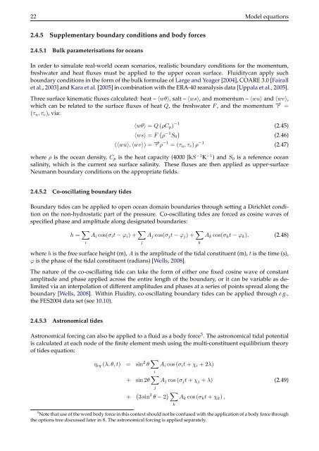
22 Model equations
2.4.5 Supplementary boundary conditions and body forces
2.4.5.1 Bulk parameterisations for oceans
In order to simulate real-world ocean scenarios, realistic boundary conditions for the momentum,
freshwater and heat fluxes must be applied to the upper ocean surface. Fluiditycan apply such
boundary conditions in the form of the bulk formulae of Large and Yeager [2004], COARE 3.0 [Fairall
et al., 2003] and Kara et al. [2005] in combination with the ERA-40 reanalysis data [Uppala et al., 2005].
Three surface kinematic fluxes calculated: heat – 〈wθ〉, salt – 〈ws〉, and momentum – 〈wu〉 and 〈wv〉,
which can be related to the surface fluxes of heat Q, the freshwater F , and the momentum −→ τ =
(τu, τv), via:
〈wθ〉 = Q (ρCp) −1
〈ws〉 = F � ρ −1 �
S0
(〈wu〉, 〈wv〉) = −→ τ ρ −1 = (τu, τv) ρ −1
(2.45)
(2.46)
(2.47)
where ρ is the ocean density, Cp is the heat capacity (4000 JkS −1 K −1 ) and S0 is a reference ocean
salinity, which is the current sea surface salinity. These fluxes are then applied as upper-surface
Neumann boundary conditions on the appropriate fields.
2.4.5.2 Co-oscillating boundary tides
Boundary tides can be applied to open ocean domain boundaries through setting a Dirichlet condition
on the non-hydrostatic part of the pressure. Co-oscillating tides are forced as cosine waves of
specified phase and amplitude along designated boundaries:
h = �
Ai cos(σit − ϕi) + �
Aj cos(σjt − ϕj) + �
Ak cos(σkt − ϕk), (2.48)
i
j
where h is the free surface height (m), A is the amplitude of the tidal constituent (m), t is the time (s),
ϕ is the phase of the tidal constituent (radians) [Wells, 2008].
The nature of the co-oscillating tide can take the form of either one fixed cosine wave of constant
amplitude and phase applied across the entire length of the boundary, or it can be variable as delimited
via an interpolation of different amplitudes and phases at a series of points spread along the
boundary [Wells, 2008]. Within Fluidity, co-oscillating boundary tides can be applied through e.g.,
the FES2004 data set (see 10.10).
2.4.5.3 Astronomical tides
Astronomical forcing can also be applied to a fluid as a body force 5 . The astronomical tidal potential
is calculated at each node of the finite element mesh using the multi-constituent equilibrium theory
of tides equation:
ηeq (λ, θ, t) = sin 2 θ �
i
Ai cos (σit + χi + 2λ)
k
+ sin 2θ �
Aj cos (σjt + χj + λ) (2.49)
j
+ � 3 sin 2 θ − 2 � �
Ak cos (σkt + χk) ,
5 Note that use of the word body force in this context should not be confused with the application of a body force through
the options tree discussed later in 8. The astronomical forcing is applied separately.
k