Chapter 8 Configuring Fluidity - The Applied Modelling and ...

28 Numerical discretisation
where we have substituted c = �
j ϕjcj. From this it is readily seen that we have in fact obtained a
matrix equation of the following form
where M, A and K are the following matrices
�
Mij =
3.2.1.3 Advective stabilisation for CG
Ω
M dc
+ A(u)c + Kc = 0, (3.8)
dt
�
�
ϕiϕj, Aij = − ∇ϕi · uϕj, Kij = ∇ϕi · µ · ∇ϕj. (3.9)
Ω
Ω
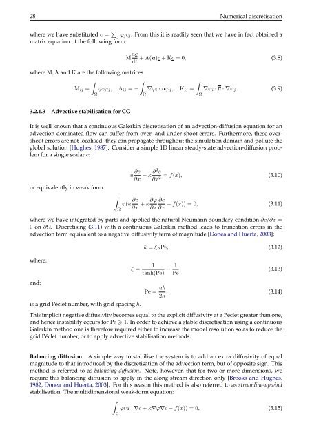
It is well known that a continuous Galerkin discretisation of an advection-diffusion equation for an
advection dominated flow can suffer from over- and under-shoot errors. Furthermore, these overshoot
errors are not localised: they can propagate throughout the simulation domain and pollute the
global solution [Hughes, 1987]. Consider a simple 1D linear steady-state advection-diffusion problem
for a single scalar c:
or equivalently in weak form:
�
Ω
u ∂c
∂x − κ ∂2c = f(x), (3.10)
∂x2 ϕ(u ∂c
∂x
∂c
+ κ∂ϕ − f(x)) = 0, (3.11)
∂x ∂x
where we have integrated by parts and applied the natural Neumann boundary condition ∂c/∂x =
0 on ∂Ω. Discretising (3.11) with a continuous Galerkin method leads to truncation errors in the
advection term equivalent to a negative diffusivity term of magnitude [Donea and Huerta, 2003]:
where:
and:
ξ =
is a grid Péclet number, with grid spacing h.
¯κ = ξκPe, (3.12)
1 1
− , (3.13)
tanh(Pe) Pe
Pe = uh
, (3.14)
2κ
This implicit negative diffusivity becomes equal to the explicit diffusivity at a Péclet greater than one,
and hence instability occurs for Pe � 1. In order to achieve a stable discretisation using a continuous
Galerkin method one is therefore required either to increase the model resolution so as to reduce the
grid Péclet number, or to apply advective stabilisation methods.
Balancing diffusion A simple way to stabilise the system is to add an extra diffusivity of equal
magnitude to that introduced by the discretisation of the advection term, but of opposite sign. This
method is referred to as balancing diffusion. Note, however, that for two or more dimensions, we
require this balancing diffusion to apply in the along-stream direction only [Brooks and Hughes,
1982, Donea and Huerta, 2003]. For this reason this method is also referred to as streamline-upwind
stabilisation. The multidimensional weak-form equation:
�
ϕ(u · ∇c + κ∇ϕ∇c − f(x)) = 0, (3.15)
Ω