Chapter 8 Configuring Fluidity - The Applied Modelling and ...

36 Numerical discretisation
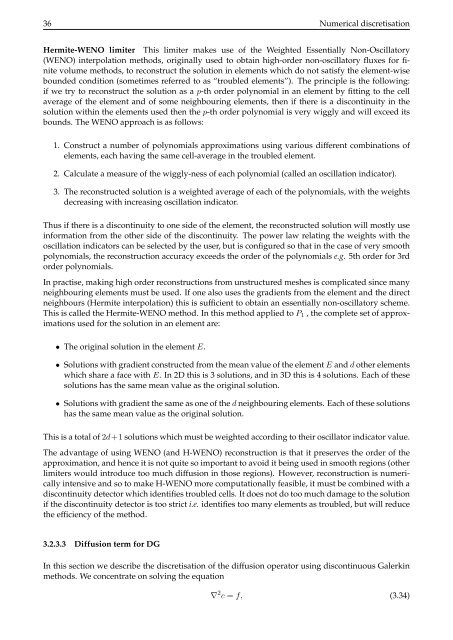
Hermite-WENO limiter This limiter makes use of the Weighted Essentially Non-Oscillatory
(WENO) interpolation methods, originally used to obtain high-order non-oscillatory fluxes for finite
volume methods, to reconstruct the solution in elements which do not satisfy the element-wise
bounded condition (sometimes referred to as “troubled elements”). The principle is the following:
if we try to reconstruct the solution as a p-th order polynomial in an element by fitting to the cell
average of the element and of some neighbouring elements, then if there is a discontinuity in the
solution within the elements used then the p-th order polynomial is very wiggly and will exceed its
bounds. The WENO approach is as follows:
1. Construct a number of polynomials approximations using various different combinations of
elements, each having the same cell-average in the troubled element.
2. Calculate a measure of the wiggly-ness of each polynomial (called an oscillation indicator).
3. The reconstructed solution is a weighted average of each of the polynomials, with the weights
decreasing with increasing oscillation indicator.
Thus if there is a discontinuity to one side of the element, the reconstructed solution will mostly use
information from the other side of the discontinuity. The power law relating the weights with the
oscillation indicators can be selected by the user, but is configured so that in the case of very smooth
polynomials, the reconstruction accuracy exceeds the order of the polynomials e.g. 5th order for 3rd
order polynomials.
In practise, making high order reconstructions from unstructured meshes is complicated since many
neighbouring elements must be used. If one also uses the gradients from the element and the direct
neighbours (Hermite interpolation) this is sufficient to obtain an essentially non-oscillatory scheme.
This is called the Hermite-WENO method. In this method applied to P1 , the complete set of approximations
used for the solution in an element are:
• The original solution in the element E.
• Solutions with gradient constructed from the mean value of the element E and d other elements
which share a face with E. In 2D this is 3 solutions, and in 3D this is 4 solutions. Each of these
solutions has the same mean value as the original solution.
• Solutions with gradient the same as one of the d neighbouring elements. Each of these solutions
has the same mean value as the original solution.
This is a total of 2d+1 solutions which must be weighted according to their oscillator indicator value.
The advantage of using WENO (and H-WENO) reconstruction is that it preserves the order of the
approximation, and hence it is not quite so important to avoid it being used in smooth regions (other
limiters would introduce too much diffusion in those regions). However, reconstruction is numerically
intensive and so to make H-WENO more computationally feasible, it must be combined with a
discontinuity detector which identifies troubled cells. It does not do too much damage to the solution
if the discontinuity detector is too strict i.e. identifies too many elements as troubled, but will reduce
the efficiency of the method.
3.2.3.3 Diffusion term for DG
In this section we describe the discretisation of the diffusion operator using discontinuous Galerkin
methods. We concentrate on solving the equation
∇ 2 c = f, (3.34)