- Page 1: Fluidity�Manual Applied Modelling
- Page 5 and 6: Contents 1 Getting started 1 1.1 In
- Page 7 and 8: CONTENTS vii 7.3 The Gmsh format .
- Page 9 and 10: CONTENTS ix 9.4.3 Stat file diagnos
- Page 11 and 12: List of Figures 2.1 Schematic of co
- Page 13 and 14: LIST OF FIGURES xiii 10.8 Schematic
- Page 15 and 16: Chapter 1 Getting started 1.1 Intro
- Page 17 and 18: 1.2 Obtaining Fluidity 3 The third,
- Page 19 and 20: 1.3 Building Fluidity 5 1.2.3.4 Oth
- Page 21 and 22: 1.3 Building Fluidity 7 1.3.2.2 Spe
- Page 23 and 24: 1.5 Running diamond 9 Signal handli
- Page 25 and 26: Chapter 2 Model equations 2.1 How t
- Page 27 and 28: 2.3 Fluid equations 13 2.2.2.2 Neum
- Page 29 and 30: 2.3 Fluid equations 15 2.3.2.2 Comp
- Page 31 and 32: 2.3 Fluid equations 17 2.3.4 Moment
- Page 33 and 34: 2.4 Extensions, assumptions and der
- Page 35 and 36: 2.4 Extensions, assumptions and der
- Page 37 and 38: 2.4 Extensions, assumptions and der
- Page 39 and 40: Chapter 3 Numerical discretisation
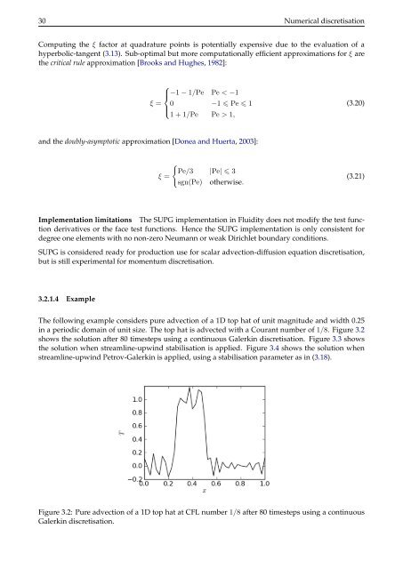
- Page 41 and 42: 3.2 Spatial discretisation of the a
- Page 43: 3.2 Spatial discretisation of the a
- Page 47 and 48: 3.2 Spatial discretisation of the a
- Page 49 and 50: 3.2 Spatial discretisation of the a
- Page 51 and 52: 3.2 Spatial discretisation of the a
- Page 53 and 54: 3.2 Spatial discretisation of the a
- Page 55 and 56: 3.2 Spatial discretisation of the a
- Page 57 and 58: 3.2 Spatial discretisation of the a
- Page 59 and 60: 3.2 Spatial discretisation of the a
- Page 61 and 62: 3.2 Spatial discretisation of the a
- Page 63 and 64: 3.3 The time loop 49 The coupled li
- Page 65 and 66: 3.4 Time discretisation of the adve
- Page 67 and 68: 3.6 Pressure equation for incompres
- Page 69 and 70: 3.7 Velocity and pressure element p
- Page 71 and 72: 3.8 Balance pressure 57 3.8 Balance
- Page 73 and 74: 3.10 Linear solvers 59 When reachin
- Page 75 and 76: 3.11 Algorithm for detectors (Lagra
- Page 77 and 78: Chapter 4 Parameterisations Althoug
- Page 79 and 80: 4.1 Generic length scale turbulence
- Page 81 and 82: 4.3 Large-Eddy Simulation (LES) 67
- Page 83 and 84: 4.3 Large-Eddy Simulation (LES) 69
- Page 85 and 86: Chapter 5 Embedded models The param
- Page 87 and 88: 5.1 Biology 73 where kN is the half
- Page 89 and 90: Chapter 6 Adaptive remeshing 6.1 Mo
- Page 91 and 92: 6.4 Metric formation 77 By contrast
- Page 93 and 94: 6.6 Related topics 79 There are two
- Page 95 and 96:
Chapter 7 Mesh generation This chap
- Page 97 and 98:
7.2 The triangle format 83 1 Rema
- Page 99 and 100:
7.3 The Gmsh format 85 three parts:
- Page 101 and 102:
7.6 Decomposing meshes for parallel
- Page 103 and 104:
7.9 Non-Fluidity tools 89 7.7 Pseud
- Page 105 and 106:
7.9 Non-Fluidity tools 91 7.9.3 Imp
- Page 107 and 108:
Chapter 8 Configuring Fluidity 8.1
- Page 109 and 110:
8.3 The options tree 95 Figure 8.2:
- Page 111 and 112:
8.3 The options tree 97 8.3.4 IO Th
- Page 113 and 114:
8.3 The options tree 99 Checkpoint
- Page 115 and 116:
8.3 The options tree 101 8.3.5.3 Fi
- Page 117 and 118:
8.4 Meshes 103 if t < 4000.0: omega
- Page 119 and 120:
8.5 Material/Phase 105 8.4.2.4 Extr
- Page 121 and 122:
8.6 Fields 107 dent field). This is
- Page 123 and 124:
8.7 Advected quantities: momentum a
- Page 125 and 126:
8.7 Advected quantities: momentum a
- Page 127 and 128:
8.9 Solution of linear systems 113
- Page 129 and 130:
8.10 Equation of State (EoS) 115 8.
- Page 131 and 132:
8.11 Subgridscale Parameterisations
- Page 133 and 134:
8.12 Boundary conditions 119 8.12.3
- Page 135 and 136:
8.12 Boundary conditions 121 • ..
- Page 137 and 138:
8.16 Large scale low aspect ratio o
- Page 139 and 140:
8.16 Large scale low aspect ratio o
- Page 141 and 142:
8.17 Geophysical fluid dynamics pro
- Page 143 and 144:
8.18 Mesh adaptivity 129 An Element
- Page 145 and 146:
8.19 Multiple material/phase models
- Page 147 and 148:
8.19 Multiple material/phase models
- Page 149 and 150:
8.20 Compressible fluid model 135 t
- Page 151 and 152:
Chapter 9 Visualisation and Diagnos
- Page 153 and 154:
9.2 Online diagnostics 139 Gravitat
- Page 155 and 156:
9.2 Online diagnostics 141 Absolute
- Page 157 and 158:
9.2 Online diagnostics 143 Figure 9
- Page 159 and 160:
9.3 Offline diagnostics 145 Program
- Page 161 and 162:
9.3 Offline diagnostics 147 Additio
- Page 163 and 164:
9.3 Offline diagnostics 149 9.3.3.1
- Page 165 and 166:
9.3 Offline diagnostics 151 Script
- Page 167 and 168:
9.3 Offline diagnostics 153 TARGET
- Page 169 and 170:
9.3 Offline diagnostics 155 Figure
- Page 171 and 172:
9.4 The stat file 157 It is also po
- Page 173 and 174:
9.4 The stat file 159 9.4.3 Stat fi
- Page 175 and 176:
Temperature min fluid .../stat/incl
- Page 177 and 178:
9.4 The stat file 163 9.4.3.1 Surfa
- Page 179 and 180:
9.4 The stat file 165 ...
- Page 181 and 182:
Chapter 10 Examples 10.1 Introducti
- Page 183 and 184:
10.2 One dimensional advection 169
- Page 185 and 186:
10.3 The lock-exchange 171 10.2.4 E
- Page 187 and 188:
10.3 The lock-exchange 173 basic se
- Page 189 and 190:
10.4 Lid-driven cavity 175 domain f
- Page 191 and 192:
10.5 Backward facing step 177 Figur
- Page 193 and 194:
10.5 Backward facing step 179 No-no
- Page 195 and 196:
10.5 Backward facing step 181 Evolu
- Page 197 and 198:
10.6 Flow past a sphere: drag calcu
- Page 199 and 200:
10.7 Rotating periodic channel 185
- Page 201 and 202:
10.8 Water column collapse 187 Exam
- Page 203 and 204:
10.8 Water column collapse 189 (a)
- Page 205 and 206:
10.8 Water column collapse 191 (a)
- Page 207 and 208:
10.9 The restratification following
- Page 209 and 210:
10.10 Tides in the Mediterranean Se
- Page 211 and 212:
10.10 Tides in the Mediterranean Se
- Page 213 and 214:
10.10 Tides in the Mediterranean Se
- Page 215 and 216:
Bibliography M. T. Ainsworth and J.
- Page 217 and 218:
C. J. Cotter, D. A. Ham, and C. C.
- Page 219 and 220:
A. Birol Kara, Harley E. Hurlburt,
- Page 221 and 222:
J. R. Shewchuk. An introduction to
- Page 223 and 224:
Appendix A About this manual A.1 In
- Page 225 and 226:
A.3 Style guide 211 The options pro
- Page 227 and 228:
A.3 Style guide 213 A.3.8.3 Derivat
- Page 229 and 230:
Appendix B Mathematical notation Th
- Page 231 and 232:
Appendix C Useful numbers The table
- Page 233 and 234:
Appendix D Dimensional analysis D.1
- Page 235 and 236:
D.2 Dimensionless parameters 221 Na
- Page 237 and 238:
Appendix E The Fluidity Python stat
- Page 239 and 240:
E.6 Debugging with an interactive P
- Page 241 and 242:
Appendix F External libraries F.1 I
- Page 243 and 244:
F.4 Manual install of external libr
- Page 245 and 246:
F.4 Manual install of external libr
- Page 247 and 248:
F.4 Manual install of external libr
- Page 249 and 250:
F.4 Manual install of external libr
- Page 251 and 252:
Appendix G Troubleshooting G.1 Back
- Page 253 and 254:
Index absorption term . . . . . . .
- Page 255:
geostrophic balance . . . . . . . .