Problemas resueltos de Cálculo Numérico

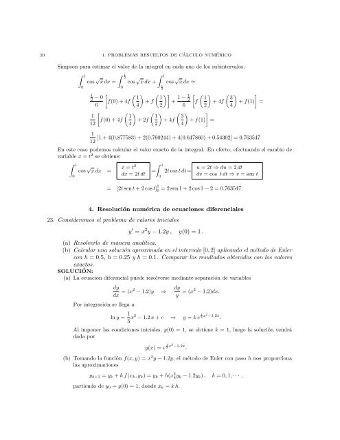
20 1. PROBLEMAS RESUELTOS DE CÁLCULO NUMÉRICO
Simpson para estimar el valor de la integral en cada uno de los subintervalos.
1
0
cos √ x dx =
1
2 − 0
6
1
12
1
2
0
f(0) + 4f
f(0) + 4f
cos √ x dx +
1
4
1
4
+ f
+ 2f
1
1
2
1
2
1
2
cos √ x dx
+ 1 − 1
2
+ 4f
6
3
4
1 3
f + 4f + f(1) =
2 4
+ f(1) =
1
[1 + 4(0.877583) + 2(0.760244) + 4(0.647860) + 0.54302] = 0.763547
12
En este caso podemos calcular el valor exacto de la integral. En efecto, efectuando el cambio de
variable x = t2 se obtiene:
1
0
cos √ x dx =
x = t 2
dx = 2t dt =
1
0
2t cos t dt=
u = 2t ⇒ du = 2 dt
dv = cos t dt ⇒ v = sen t
= [2t sen t + 2 cos t] 1
0 = 2 sen 1 + 2 cos 1 − 2 = 0.763547.
4. Resolución numérica de ecuaciones diferenciales
23. Consideremos el problema de valores iniciales
y ′ = x 2 y − 1.2y , y(0) = 1 .
(a) Resolverlo de manera analítica.
(b) Calcular una solución aproximada en el intervalo [0, 2] aplicando el método de Euler
con h = 0.5, h = 0.25 y h = 0.1. Comparar los resultados obtenidos con los valores
exactos.
SOLUCIÓN:
(a) La ecuación diferencial puede resolverse mediante separación de variables
Por integración se llega a
dy
dx = (x2 − 1.2)y ⇒ dy
y = (x2 − 1.2)dx.
ln y = 1
3 x2 − 1.2 x + c ⇒ y = k e 1
3 x2 −1.2x .
Al imponer las condiciones iniciales, y(0) = 1, se obtiene k = 1, luego la solución vendrá
dada por
y(x) = e 1
3 x2 −1.2x .
(b) Tomando la función f(x, y) = x 2 y − 1.2y, el método de Euler con paso h nos proporciona
las aproximaciones
yk+1 = yk + h f(xk, yk) = yk + h(x 2 kyk − 1.2yk) , k = 0, 1, · · · ,
partiendo de y0 = y(0) = 1, donde xk = k h.