Problemas resueltos de Cálculo Numérico

TEMA 1
Problemas resueltos de Cálculo Numérico
1. Interpolación y aproximación
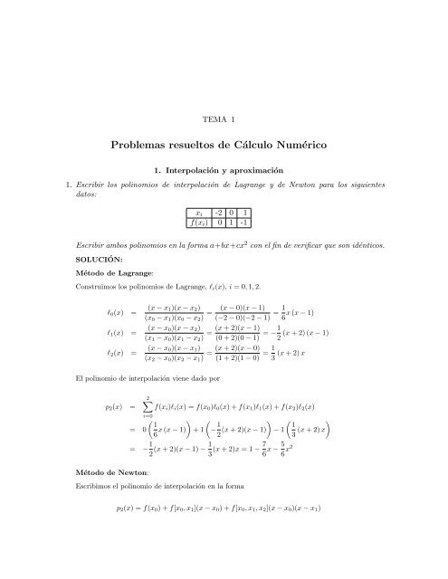
1. Escribir los polinomios de interpolación de Lagrange y de Newton para los siguientes
datos:
xi -2 0 1
f(xi) 0 1 -1
Escribir ambos polinomios en la forma a+bx+cx 2 con el fin de verificar que son idénticos.
SOLUCIÓN:
Método de Lagrange:
Construimos los polinomios de Lagrange, ℓi(x), i = 0, 1, 2.
ℓ0(x) =
ℓ1(x) =
ℓ2(x) =
(x − x1)(x − x2) (x − 0)(x − 1)
=
(x0 − x1)(x0 − x2) (−2 − 0)(−2 − 1)
1
= x (x − 1)
6
(x − x0)(x − x2) (x + 2)(x − 1)
= = −1 (x + 2) (x − 1)
(x1 − x0)(x1 − x2) (0 + 2)(0 − 1) 2
(x − x0)(x − x1) (x + 2)(x − 0) 1
= = (x + 2) x
(x2 − x0)(x2 − x1) (1 + 2)(1 − 0) 3
El polinomio de interpolación viene dado por
p2(x) =
= 0
2
f(xi)ℓi(x) = f(x0)ℓ0(x) + f(x1)ℓ1(x) + f(x2)ℓ2(x)
i=0
= − 1
2
Método de Newton:
1
x (x − 1)
6
(x + 2)(x − 1) − 1
3
+ 1 − 1
(x + 2)(x − 1)
2
Escribimos el polinomio de interpolación en la forma
7 5
(x + 2)x = 1 − x −
6 6 x2
1
− 1 (x + 2) x
3
p2(x) = f(x0) + f[x0, x1](x − x0) + f[x0, x1, x2](x − x0)(x − x1)

2 1. PROBLEMAS RESUELTOS DE CÁLCULO NUMÉRICO
Calculamos la tabla de diferencias divididas
Luego,
p2(x) = 0 + 1
2
xi f(xi
-2 0
1/2
0 1 -5/6
-2
1 -1
(x + 2) − 5
6
7 5
(x + 2)(x − 0) = 1 − x −
6 6 x2
2. Determinar un polinomio p(x) = ax 6 + bx 4 + cx 2 + d que satisfaga los siguientes datos
SOLUCIÓN:
p(0) = 2 , p(−1) = 8 , p ′′ (0) = −2 , p ′′ (−1) = 8 .
p(x) = a x 6 + b x 4 + c x 2 + d
p ′ (x) = 6a x 5 + 4b x 3 + 2c x
p ′′ (x) = 30a x 4 + 12b x 2 + 2c
Al imponer las condiciones de interpolación se tiene
p(0) = 2 ⇒ d = 2
p(−1) = 8 ⇒ a + b + c + d = 8
p ′′ (0) = 2 ⇒ 2c = 2
Resolviendo el sistema anterior obtenemos
El polinomio pedido será
p ′′ (−1) = 8 ⇒ 30a + 12b + 2c = 8
a = − 37
9
100
, b = , c = −1, d = 2.
9
p(x) = − 37
6 x6 + 100
9 x4 − x 2 + 2.
3. En estudios de polimerización inducida por radiación, se emplea una fuente de rayos
gamma para obtener dosis medidas en radiación. Sin embargo, la dosis varía con la
posición del aparato, según los datos que se dan a continuación.
Posición Dosis
(en pulgadas) (10 5 rads/h)
1.0 2.71
1.5 2.98
2.0 3.20
3.0 3.20
(a) ¿Cuál es la estimación para el nivel de dosis en 2.5 pulgadas?

1. INTERPOLACIÓN Y APROXIMACIÓN 3
(b) Si se efectúa una nueva medición que indica que a 3.5 pulgadas el nivel de dosis
correspondiente es de 2 ′ 98, ¿cuál será ahora la estimación para el nivel de dosis en
2.5 pulgadas?
SOLUCIÓN:
(a) Calculamos el polinomio de interpolación para los datos de la tabla anterior. Utilizamos el
método de Newton.
xi f(xi)
1.0 2.71
0.54
1.5 2.98 -0.1
0.44 -0.29/3
2.0 3.20 -0.44/1.5
0
3.0 3.20
El polinomio de interpolación vendrá dado por
p3(x) = 2.71 + 0.54(x − 1) − 0.1(x − 1)(x − 1.5) − 0.29
(x − 1)(x − 1.5)(x − 2).
3
Ahora podemos estimar la dosis de radiación para x = 2.5 evaluando el polinomio de
interpolación en ese punto.
p3(2.5) = 2.71 + 0.54(1.5) − 0.1(1.5)(1) − 0.29
(1.5)(0.5) = 3.2975.
3
(b) Observemos que ahora disponemos de un dato más de interpolación. Una forma de obtener
el nuevo polinomio de interpolación es añadir este dato a nuestra tabla de diferencias divididas
y completarla.
xi f(xi)
1.0 2.71
0.54
1.5 2.98 -0.1
0.44 -0.29/3
2.0 3.20 -0.44/1.5 0.29/7.5
0 0
3.0 3.20 -0.44/1.5
-0.44
3.5 2.98
El nuevo polinomio de interpolación será
p4(x) = 2.71 + 0.54(x − 1) − 0.1(x − 1)(x − 1.5) −
0.29
(x − 1)(x − 1.5)(x − 2) +
3
0.29
(x − 1)(x − 1.5)(x − 2)(x − 3).
7.5
La estimación del nivel de radiación para x = 2.5 será ahora
p4(2.5) = 3.2975 + 0.29
(1.5)(0.5)(−0.5) = 3.283
7.5

4 1. PROBLEMAS RESUELTOS DE CÁLCULO NUMÉRICO
4. Para los valores siguientes
E 40 60 80 100 120
P 0.63 1.36 2.18 3.00 3.93
donde E son los voltios y P los kilovatios en una curva de pérdida en el núcleo para un
motor eléctrico.
(a) Elaborar una tabla de diferencias divididas
(b) Calcular el polinomio de interpolación de Newton de segundo grado para E =
80, 100, 120. Utilizarlo para estimar el valor de P correspondiente a E = 90 voltios.
SOLUCIÓN:
(a) Calculamos la tabla de diferencias divididas
xi f(xi)
40 0.63
0.0365
60 1.36 0.0001125
0.041 -0.000001875
80 2.18 0 0.0000000521
0.041 0.00002292
100 3.00 0.0001375
0.0465
120 3.93
(b) En la tabla anterior hemos marcado los coeficientes del polinomio de interpolación para
E = 80, 100, 120. El polinomio será
p2(x) = 2.18 + 0.041(x − 80) + 0.0001375(x − 80)(x − 100).
La estimación de P para E = 90 se obtendrá evaluando el polinomio de interpolación en
x = 90. En nuestro caso
p(90) = 2.18 + 0.041(10) + 0.0001375(10)(−10) = 2.57625
5. Una función f(x) de la que solamente se conocen los datos de la tabla que figura a continuación,
alcanza un máximo en el intervalo [1, 1.3]. Hallar la abscisa de dicho máximo.
Interpreta los resultados.
SOLUCIÓN:
xi 1.0 1.1 1.2 1.3
f(xi) 0.841 0.891 0.993 1.000
La solución de este problema pasa necesariamente por determinar una función que interpole o
aproxime los datos anteriores. A continuación calculamos el punto donde esta función alcance
su máximo o su mínimo. Por tanto, una primera estrategia puede ser calcular el polinomio de
interpolación.

El polinomio de interpolación será
1. INTERPOLACIÓN Y APROXIMACIÓN 5
xi f(xi)
1.0 0.841
0.5
1.1 0.891 2.6
1.02 -24.5
1.2 0.993 -4.75
0.07
1.3 1.00
p(x) = 0.841 + 0.5(x − 1) + 2.6(x − 1)(x − 1.1) − 24.5(x − 1)(x − 1.1)(x − 1.2)
= 35.541 − 93.65x + 83.45x 2 − 24.5x 3
Calculamos los puntos críticos
p ′ (x) = 0 ⇒ −73.5x 2 + 166.9x − 93.65 = 0 ⇒
x = 1.25754
x = 1.01321
Para precisar si hay máximo o mínimo recurrimos a la segunda derivada.
p ′′ (x) = −147x + 166.9 ⇒
Puesto que
p ′′ (1.25754) = −17.95838 < 0 ⇒ máx. relativo
p ′′ (1.01321) = 17.95813 > 0 ⇒ mín. relativo
p(1.25754) = 1.018062648073915
deducimos que la función p(x) alcanza su máximo absoluto en el intervalo [1, 1.3] en el punto de
abscisa x = 1.25754.
Otra forma de abordar este problema sería utilizando interpolación lineal a trozos. De acuerdo
con este nuevo modelo y observando los datos de la tabla anterior concluiríamos que la función
f(x) alcanzaría su máximo absoluto en x = 1.30.
6. En la siguiente tabla, R es la resistencia de una bobina en ohms y T la temperatura de
la bobina en grados centígrados. Por mínimos cuadrados determinar el mejor polinomio
lineal que represente la función dada.
SOLUCIÓN:
T 10.50 29.49 42.70 60.01 75.51 91.05
R 10.421 10.939 11.321 11.794 12.242 12.668
Se trata de ajustar una función del tipo
R = a + b T
al conjunto de datos (Ti, Ri). Matricialmente el sistema que tenemos que resolver vendrá dado
por
⎛ 6 6
⎞ ⎛ 6
⎞
⎜ 1 Ti ⎟ ⎜ Ri ⎟
⎜
⎟
⎜ i=1 i=1 a ⎜ ⎟
⎟
⎜ 6 6
⎟ = ⎜ i=1 ⎟
⎝
⎠ b ⎜ 6
⎟
⎝ ⎠
i=1
Ti
i=1
T 2 i
i=1
TiRi

6 1. PROBLEMAS RESUELTOS DE CÁLCULO NUMÉRICO
Construimos la siguiente tabla
Ti Ri T 2 i TiRi
10.50 10.421 110.25 109.4205
29.49 10.939 869.6501 322.59111
42.70 11.321 1823.29 483.4067
60.01 11.794 3601.2001 707.75794
75.51 12.242 5701.7601 924.39242
91.05 12.668 8290.1025 1153.4214
309.26 69.385 20396.2628 3700.99107
Por tanto, el sistema que tenemos que resolver será,
6a + 309.26b = 69.385
309.26a + 20396.2628b = 3700.99107 ⇒
Luego, la solución vendrá dada por
R = 10.1222293891 + 0.0279752430495 T
a = 10.1222293891
b = 0.0279752430495
7. Aproximar mediante los mínimos cuadrados un polinomio de grado dos a los siguientes
datos
xi 1 2 4 10 16
yi 6 1 2 4 5
SOLUCIÓN:
Se trata de ajustar una función del tipo
i=1
x 2 i
i=1
x 3 i
y = a + b x + c x 2
al conjunto de datos (xi, yi).
Matricialmente el sistema que tenemos que resolver vendrá dado por
⎛
5 5 5
⎜ 1 xi x
⎜ i=1 i=1 i=1
⎜
⎝
2 i
5 5
xi x
i=1 i=1
2 5
i x
i=1
3 ⎞ ⎛ 5
⎞
⎟ ⎜ yi ⎟
⎟ ⎛ ⎞ ⎜ ⎟
⎜ i=1 ⎟
⎟ a ⎜
⎟ ⎜ ⎟ ⎜ 5
⎟
i ⎟ ⎝ b ⎠ = ⎜ xiyi
⎟
⎟ ⎜
5 5 5
⎟ c
i=1 ⎟
⎜ ⎟
⎟ ⎜ 5 ⎟
⎠ ⎝ ⎠
Construimos la siguiente tabla
i=1
x 4 i
i=1
xi yi x 2 i x 3 i x 4 i xiyi x 2 i yi
1 6 1 1 1 6 6
2 1 4 8 16 2 4
4 2 16 64 256 8 32
10 4 100 1000 10000 40 400
16 5 256 4096 65536 80 1280
33 18 377 5169 75809 136 1722
x 2 i yi

1. INTERPOLACIÓN Y APROXIMACIÓN 7
Por tanto, el sistema que tenemos que resolver será,
⎧
⎨
⎩
5a + 33b + 377c = 18
33a + 377b + 5169c = 136
377a + 5169b + 75809c = 1722
Luego, la solución vendrá dada por
8. Hallar la función del tipo
⇒
⎧
⎨
⎩
y = 4.08582 − 0.45685x + 0.03355x 2
a = 4.08582
b = −0.45685
c = 0.03355
g(x) = a √ x + b
x
que mejor se ajuste, mediante el criterio de los mínimos cuadrados, a los datos
SOLUCIÓN:
(1, 2) , (2, 4) , (3, 0).
Matricialmente el sistema que tenemos que resolver vendrá dado por
⎛
⎜
⎝
3
xi
i=1
3
3 1
√
xi
i=1
3 1
⎞ ⎛
⎟ ⎜
⎟ a ⎜
⎟ = ⎜
⎠ b ⎜
⎝
3 √
xi yi
i=1
3 1
⎞
⎟
⎠
i=1
√ xi
x
i=1
2 i
yi
xi
i=1
Construimos la siguiente tabla
xi 1/ √ xi 1/x2 1 1
i
1
√
xi yi
2
yi/xi
2
2 0.7071 0.25 5.65685 2
4 0.5 0.0625 0 0
7 2.20711 1.3125 7.65685 4
Por tanto, el sistema que tenemos que resolver será,
7a + 2.20711b = 7.65685
2.20711a + 1.3125b = 4
Luego, la solución vendrá dada por
⇒
y = 0.43556 √ x + 2.20774
x
.
a = 0.43556
b = 2.20774
9. En la siguiente tabla aparecen recogidos los datos de población de un pequeño barrio de
una ciudad en un periodo de 20 años. Como ingeniero que trabaja en una compañía de
servicio debes pronosticar la población que habrá dentro de 5 años, para poder anticipar
la demanda de energía. Emplea un modelo exponencial y regresión lineal para hacer esta
predicción.
t 0 5 10 15 20
p 100 212 448 949 2009

8 1. PROBLEMAS RESUELTOS DE CÁLCULO NUMÉRICO
SOLUCIÓN:
Pretendemos ajustar una función del tipo
p = a e bt .
Se trata de un modelo de aproximación no lineal. Tomando logaritmos y denotando P = ln p y
A = ln a se llega al modelo lineal
ln p = ln a e bt = ln a + b t ⇒ P = A + b t.
Ahora nuestro objetivo será ajustar una función del tipo P = A + b t al conjunto de datos (ti, Pi).
Matricialmente el sistema que tenemos que resolver será
⎛ 5 5
⎞ ⎛ 5
⎞
⎜ 1 ti ⎟ ⎜ Pi ⎟
⎜
⎟
⎜ i=1 i=1 A ⎜ ⎟
⎟
⎜ 5 5
⎟ = ⎜ i=1 ⎟
⎝
⎠ b ⎜ 6
⎟
⎝ ⎠
i=1
Construimos la siguiente tabla
ti
i=1
t 2 i
i=1
tiPi
ti pi Pi = ln pi t 2 i tiPi
0 100 4.6052 0 0
5 212 5.3566 25 26.783
10 448 6.1048 100 61.048
15 949 6.8554 225 102.831
20 2009 7.6054 400 152.108
50 30.5274 750 342.77
Por tanto, el sistema que tenemos que resolver será,
5A + 50b = 30.5274
50A + 750b = 342.77 ⇒
A 4.60564 A = 4.60564 ⇒ a = e = e = 100.0470
b = 0.149984
Luego, la solución vendrá dada por
p(t) = 100.0470 e 0.149984 t .
La población estimada en los próximos 5 años se obtendrá calculando p(25). En nuestro caso,
p(25) = 100.0470e 3.7496 4252.
2. Resolución numérica de ecuaciones
10. Probar que la ecuación
e x − 2e −x = 0
tiene una única solución real. Obtenerla mediante el método de Newton-Raphson (3 iteraciones).
Utiliza 5 cifras decimales en los cálculos.
SOLUCIÓN:
Consideramos la función
f(x) = e x − 2e −x .
Buscamos un intervalo donde haya alternancia de signo
f(0) = −1 , f(1) = 1.9825

2. RESOLUCIÓN NUMÉRICA DE ECUACIONES 9
Puesto que f es una función continua, el teorema de Bolzano nos garantiza la existencia de al
menos una solución en el intervalo (0, 1). Además se tiene que
por lo que la solución es única.
f ′ (x) = e x + 2e −x = 0 , ∀x ∈ IR,
Apliquemos el método de Newton para obtener de forma aproximada la solución.
xn+1 = xn − f(xn)
f ′ , n ≥ 0.
(xn)
Elegimos como punto de arranque un x0 ∈ [0, 1] tal que f(x0)f ′′ (x0) > 0. En este caso, puesto
que
f ′′ (x) = e x − 2e −x ,
podemos tomar como punto de arranque cualquier x0 ∈ [0, 1].
Partiendo de x0 = 0 generamos las siguientes aproximaciones
x0 = 0
x1 = x0 − f(x0)
f ′ f(0)
= 0 −
(x0) f ′ = −−1 = 0.33333
(0) 3
x2 = x1 − f(x1)
f ′ f(0.33333)
= 0.33333 −
(x1) f ′ = 0.34654
(0.33333)
x3 = x2 − f(x2)
f ′ f(0.34654)
= 0.34654 −
(x2) f ′ = 0.34657
(0.34654)
En este caso, podemos resolver algebraicamente la ecuación para obtener la solución exacta.
e x − 2e −x = 0 ⇒ e 2x − 2 = 0 ⇒ x = 1
ln 2 = 0.346573590279972
2
11. Aproximar mediante el método de la regula falsi la raíz de la ecuación
x 3 − 2x 2 − 5 = 0
en el intervalo [1, 4], realizando 5 iteraciones y utilizando cinco cifras decimales.
SOLUCIÓN:
Definimos la función f(x) = x 3 − 2x 2 − 5. Puesto que f(1) = −6 y f(4) = 27, el teorema de
Bolzano nos garantiza la existencia de al menos una solución en el intervalo (1, 4). Además, puesto
que
f ′′ (x) = 6x − 4 > 0 , ∀x ∈ [1, 4],
la función f es convexa en [1, 4]. Esto nos asegura que hay solución única en [1, 4] y que el método
de regula falsi es convergente. Generamos las aproximaciones
xn = an − f(an)(bn − an)
f(bn) − f(an)
, n = 0, 1, · · ·

10 1. PROBLEMAS RESUELTOS DE CÁLCULO NUMÉRICO
partiendo de a0 = 1, b0 = 4. Los valores an y bn se eligen en cada paso de forma que f(an)f(bn) <
0. Los cálculos realizados se recogen en la siguiente tabla.
La solución vendrá dada por
n an bn xn f(an) f(bn) f(xn)
0 1.0000 4.0 1.5454 -6.0000 27.0 -6.0856
1 1.5454 4.0 1.9969 -6.0856 27.0 -5.0122
2 1.9969 4.0 2.3105 -5.0122 27.0 -3.3420
3 2.3105 4.0 2.4966 -3.3420 27.0 -1.9043
4 2.4966 4.0 2.5957 -1.9043 27.0 -0.98648
5 2.5957 4.0 2.6452 -0.98648 27.0 -0.48559
x 2.6452
Observación: Si nos fijamos en la tabla anterior se observa que en cualquier iteración, bn = b0
y an+1 = xn. Esta situación se podía haber previsto inicialmente por la convexidad de la función
f. De esta forma las aproximaciones se podrían calcular directamente a partir de la fórmula
xn = xn−1 − f(xn−1)(b − xn−1)
f(b) − f(xn−1)
, n = 0, 1, · · ·
tomando x−1 = a0 = 1.
12. Encontrar un valor aproximado de 3√ 2 mediante el método de bisección y el método de la
secante.
SOLUCIÓN:
Consideramos la función f(x) = x 3 − 2 y buscamos un intervalo donde haya alternancia de signo
f(1) = −1 , f(1.5) = 1.375
El teorema de Bolzano nos garantiza la existencia de al menos una solución en el intervalo [1, 1.5].
Además, puesto que
f ′ (x) = 3x 2 = 0 , ∀x ∈ [1, 1.5]
la solución será única.
Método de bisección: Partiendo de a0 = 1, b0 = 1.5 generamos las aproximaciones
xn = an + bn
2
donde an y bn se eligen de forma que en cualquier iteración se cumpla que f(an)f(bn) < 0. Los
cálculos efectuados se recogen en la siguiente tabla
n an bn xn f(an) f(bn) f(xn)
0 1.0 1.5 1.25 -1.000 1.375 -0.046
1 1.25 1.5 1.375 -0.046 1.375 0.599
2 1.25 1.375 1.3125 -0.046 0.599 0.260
3 1.25 1.3125 1.28125 -0.046 0.260 0.103
4 1.25 1.28125 1.265625 -0.046 0.103 0.0272
5 1.25 1.265625 1.2578125 -0.046 0.027 -0.01
6 1.2578125 1.265625 1.26171875 -0.010 0.027 0.008
7 1.2578125 1.26171875 1.259765625 -0.010 0.008 -0.0007
8 1.259765625 1.26171875 1.2607421875 -0.0007 0.008 0.003
9 1.259765625 1.2607421875 1.26025390625 -0.0007 0.003 0.001
10 1.259765625 1.26025390625 1.260009765625 -0.0007 0.001 0.0004

2. RESOLUCIÓN NUMÉRICA DE ECUACIONES 11
El valor aproximado obtenido después de 10 iteraciones del método de bisección es
x 1.260009765625
Método de la secante: Partiendo de x0 = 1 y x1 = 1.5 generamos las aproximaciones
xn+1 = xn − f(xn)(xn − xn−1)
f(xn) − f(xn−1)
x0 = 1
x1 = 1.5
x2 = x1 − f(x1)(x1 − x0)
f(x1) − f(x0)
x3 = x2 − f(x2)(x2 − x1)
f(x2) − f(x1)
x4 = x3 − f(x3)(x3 − x2)
f(x3) − f(x2)
x5 = x4 − f(x4)(x4 − x3)
f(x4) − f(x3)
x6 = x5 − f(x5)(x5 − x4)
f(x5) − f(x4)
, n = 1, 2, · · ·
= 1.2105263157894736842
= 1.2514085388756729685
= 1.2602652758390120360
= 1.2599187140887994992
= 1.2599210492568176179
La solución aproximada obtenida al realizar 5 iteraciones con el método de la secante viene dada
por
x 1.2599210492568176179
13. Determinar una solución aproximada de la ecuación
ln x − x + 2 = 0
en el intervalo [3, 4], utilizando 3 iteraciones con el método de Newton-Raphson.
SOLUCIÓN:
Puesto que f es continua en el intervalo [3, 4] y f(3)f(4) < 0, el teorema de Bolzano nos garantiza
la existencia de al menos una solución en dicho intervalo. Además,
f ′ (x) = 1
− 1 = 0 , ∀x ∈ [3, 4],
x
lo que nos asegura que hay solución única en el intervalo [3, 4].
Generamos las aproximaciones de la solución mediante el algoritmo
xn+1 = xn − f(xn)
f ′ , n = 0, 1, · · ·
(xn)

12 1. PROBLEMAS RESUELTOS DE CÁLCULO NUMÉRICO
partiendo de un punto inicial x0 ∈ [3, 4] tal que f(x0)f ′′ (x0) > 0. Puesto que f ′′ (x) = −1/x 2
podemos tomar como punto de arranque x0 = 4.
x0 = 4
x1 = x0 − f(x0)
f ′ f(4)
= 4 −
(x0) f ′ = 3.181725815
(4)
x2 = x1 − f(x1)
f ′ f(3.181725815)
= 3.181725815 −
(x1) f ′ = 3.146284844
(3.181725815)
x3 = x2 − f(x2)
f ′ f(3.146284844)
= 3.146284844 −
(x2) f ′ = 3.146193221
(3.146284844)
14. Resolver la ecuación diferencial
SOLUCIÓN:
y ′′′ + y ′′ − 3y ′ − y = 0.
El conjunto fundamental de soluciones de la ecuación diferencial anterior se obtiene resolviendo
la ecuación característica
r 3 + r 2 − 3r − 1 = 0.
Dado que la ecuación es polinómica de grado impar sabemos que tiene al menos una solución
real. Las posibles soluciones racionales de esta ecuación son ±1. La comprobación mediante la
regla de Ruffini nos revela que ninguna de ellas es solución. Hemos de buscar, por tanto, raíces
irracionales. En este caso, la regla de Ruffini no es operativa. Afortunadamente podemos obtener
una solución aproximada utilizando el método de Newton-Raphson.
Comenzamos definiendo la función f(r) = r 3 + r 2 − 3r − 1 y buscamos un intervalo donde haya
alternancia de signo.
f(1) = −2 , f(2) = 5
Tenemos, por tanto, asegurada la existencia de solución en el intervalo [1, 2]. Además,
f ′ (r) = 3r 2 + 2r − 3
cuyas raíces son −1.38742588672 y 0.72075922005, por lo que f ′ (x) = 0, ∀x ∈ [1, 2]. Esto nos
garantiza que la solución en [1, 2] es única. Generamos las aproximaciones
rn+1 = rn − f(rn)
f ′ , n = 0, 1, · · ·
(rn)
partiendo de un punto r0 ∈ [1, 2] tal que f(r0)f ′′ (r0) > 0.

2. RESOLUCIÓN NUMÉRICA DE ECUACIONES 13
Puesto que f ′′ (r) = 6r − 2, entonces f(2)f ′′ (2) > 0. Podemos tomar r0 = 2.
r0 = 2
r1 = r0 − f(r0)
f ′ f(2)
= 2 −
(r0) f ′ = 1.6153846154
(2)
r2 = r1 − f(r1)
f ′ f(1.6153846154)
= 1.6153846154 −
(r1) f ′ = 1.4939568508
(1.6153846154)
r3 = r2 − f(r2)
f ′ f(1.4939568508)
= 1.4939568508 −
(r2) f ′ = 1.4813275882
(1.4939568508)
r4 = r3 − f(r3)
f ′ f(1.4813275882)
= 1.4813275882 −
(r3) f ′ = 1.4811943189
(1.4813275882)
r5 = r4 − f(r4)
f ′ f(1.4811943189)
= 1.4811943189 −
(r4) f ′ = 1.4811943041
(1.4811943189)
r6 = r5 − f(r5)
f ′ f(1.4811943041)
= 1.4811943041 −
(r5) f ′ = 1.48119430409
(1.4811943041)
Podemos tomar como solución r 1.48119430409. Ahora para determinar las otras soluciones
aplicamos la regla de Ruffini
1 1 -3 -1
1.48119430409 1.48119430409 3.67513087056 0.999999999989
1 2.48119430409 0.67513087056 -0.000000000011
y resolvemos la ecuación
r 2 + 2.48119430409r + 0.67513087056 = 0 ⇒
La solución general de la ecuación diferencial será
r = −0.31110781746
r = −2.17008648663
y = c1e 1.48119430409x + c2e −0.31110781746x + c3e −2.17008648663x , c1, c2, c3 ∈ IR .
15. La velocidad hacia arriba de un cohete se puede calcular usando la siguiente fórmula
v = u ln m0
− g t,
m0 − q t
donde v = velocidad hacia arriba, u = la velocidad con la que el combustible sale relativa
al cohete, m0 = masa inicial del cohete en el tiempo t = 0, q = razón de consumo de
combustible y g = aceleración hacia abajo debido a la gravedad (considérese la gravedad
constante = 9.8 m/s 2 ). Si u = 2200 m/s, m0 = 160000 Kg y q = 2680 Kg/s, calcule el
tiempo para el cual v = 1000 m/s.
SOLUCIÓN:
Se trata de resolver la ecuación
160000
1000 = 2200 ln
− 9.8 t
160000 − 2680 t
Simplificando se llega a la ecuación equivalente
Definimos la función
0.00445454545454 t + ln(4000 − 67 t) − 7.83950418556 = 0 .
f(t) = 0.00445454545454 t + ln(4000 − 67 t) − 7.83950418556

14 1. PROBLEMAS RESUELTOS DE CÁLCULO NUMÉRICO
y buscamos un intervalo donde haya alternancia de signo
f(25) = 0.0233348 , f(26) = −0.00145126.
Luego existe una solución en el intervalo [25, 26]. Además,
f ′ [t] = 0.00445454545454 −
lo que nos asegura que la solución buscada es única.
Generamos las aproximaciones mediante el algoritmo
67
= 0 , ∀t > 0,
4000 − 67t
tn+1 = tn − f(tn)
f ′ , n = 0, 1, · · ·
(tn)
partiendo de un punto inicial t0 ∈ [25, 26] tal que f(t0)f ′′ (t0) > 0. En nuestro caso f ′′ (t) =
−4489/(4000 − 67t) 2 , por lo que f(26)f ′′ (26) > 0 y podemos tomar, t0 = 26.
t0 = 26
t1 = t0 − f(t0)
f ′ f(26)
= 26 −
(t0) f ′ = 25.9424508478
(26)
t2 = t1 − f(t1)
f ′ f(25.9424508478)
= 25.9424508478 −
(t1) f ′ = 25.9423929821
(25.9424508478)
t3 = t2 − f(t2)
f ′ f(25.9423929821)
= 25.9423929821 −
(t2) f ′ = 25.9423929820
(25.9423929821)
La solución aproximada será t 25.9423929820.
3. Derivación e Integración Numérica
16. Obtener la derivada segunda en x = 3.7 para la función f(x) de la que se conocen los
siguientes datos
xi 1 1.8 3 4.2 5
f(xi) 3.00 4.34 6.57 8.88 10.44
SOLUCIÓN:
Calculamos el polinomio de interpolación de la función f para el conjunto de datos.
xi f(xi)
1.0
1.8
3.0
4.2
5.0
3.00
4.34
6.57
8.88
10.44
1.675
1.85833
1.925
1.95
0.0916667
0.027778
0.0125
-0.0199653
-0.00477431
0.00379774
El polinomio de interpolación vendrá dado por
p(x) = 3 + 1.675(x − 1) + 0.0916667(x − 1)(x − 1.8) −
0.0199653(x − 1)(x − 1.8)(x − 3) +
0.00379774(x − 1)(x − 1.8)(x − 3)(x − 4.2)
= 1.68395 + 1.03148 x + 0.338715 x 2 − 0.0579427 x 3 + 0.00379774 x 4

3. DERIVACIÓN E INTEGRACIÓN NUMÉRICA 15
Ahora podemos estimar el valor de f ′′ (3.7) evaluando p ′′ (3.7). En nuestro caso,
Luego,
p ′ (x) = 1.03148 + 0.677431 x − 0.173838 x 2 + 0.05191 x 3
p ′′ (x) = 0.677431 − 0.347656 x + 0.0455729 x 2
f ′′ (3.7) 0.677431 − 0.347656 (3.7) + 0.0455729 (3.7) 2 = 0.0149917
17. Dado un circuito con un voltaje V (t), una inductancia L y una resistencia R, la primera
ley de Kirchoff que lo modela es
V = L dI
+ RI.
dt
La siguiente tabla recoge los valores experimentales de I correspondientes a varios tiempos
t dados en segundos.
Si la inductancia L es constante e igual a 0.97 henrios y la resistencia R es de 0.14
ohmios, aproximar el voltaje V cuando t = 0.97.
SOLUCIÓN:
t 0.95 0.96 0.97 0.98 0.99 1.0
I 0.90 1.92 2.54 2.88 3.04 3.10
Dado que conocemos I(0.97) = 2.54, el problema se reduce a calcular I ′ (0.97). Para ello calculamos
el polinomio de interpolación p(t) para el conjunto de datos de la tabla anterior. La derivada de
este polinomio para t = 0.97 nos dará una estimación de I ′ (0.97).
ti
Ii
0.95 0.90
102
0.96 1.92 -2000
62 2000
0.97 2.54 -1400 -250000/3
34 50000/3 0
0.98 2.88 -900 -250000/3
16 40000/3
0.99 30.4 -500
6
1.00 3.10
El polinomio de interpolación vendrá dado por
Luego,
p(t) = 0.90 + 102(t − 0.95) − 2000(t − 0.95)(t − 0.96) +
20000(t − 0.95)(t − 0.96)(t − 0.97) −
250000
(t − 0.95)(t − 0.96)(t − 0.97)(t − 0.98)
3
= −91858.4 + 358719.83 t − 525191.67 t 2 + 341666.67 t 3 − 250000
t
3
4 .
p ′ (t) = 358719.83 − 1050383.33 t + 1025000 t 2 − 333333.33 t 3
Evaluando en t = 0.97 se tiene
I ′ (0.97) p ′ (0.97) = 358719.83 − 1050383.33 (0.97) + 1025000 (0.97) 2 −
333333.33 (0.97) 3 = 46.1667

16 1. PROBLEMAS RESUELTOS DE CÁLCULO NUMÉRICO
Por tanto,
V (0.97) = 0.97 I ′ (0.97) + 0.14 I(0.97) = 0.97(46.1667) + 0.14(2.54) = 45.1373
18. Utilizar la fórmulas usuales de derivación numérica para calcular un valor aproximado de
la derivada de la función f(x) = (1 + x)e x en el punto x = 0.6 para h = 0.1, 0.01, 0.001.
Comparar los resultados obtenidos con el valor exacto.
SOLUCIÓN:
En nuestro caso se tiene que
Por tanto,
f ′ (x) = e x + (1 + x)e x = (2 + x)e x .
f ′ (0.6) = (2 + 0.6)e 0.6 = 4.737508881015323
Al aplicar la fórmulas de derivación numérica se obtiene
f ′ (0.6)
f(0.6 + h) − f(0.6)
h
h Valor aproximado Error
0.1 5.0798952207499504 −0.3423863397346274
0.01 4.7704471413621885 −0.032938260346865533
0.001 4.7407900922387114 −0.003281211223388425
f ′ (0.6)
f(0.6 + h) − f(0.6 − h)
2h
h Valor aproximado Error
0.1 4.7514884832480853 −0.013979602232762289
0.01 4.7376485777921973 −0.00013969677687430959
0.001 4.7375102779729783 −0.13969576553307661 × 10 −5
f ′ (0.6)
4f(0.6 + h) − 3f(0.6) − f(0.6 + 2h)
2h
h Valor aproximado Error
0.1 4.7068724881917579 0.030636392823565117
0.01 4.7372269244113419 0.00028195660398111499
0.001 4.7375060845467054 0.27964686175607767 × 10 −5

3. DERIVACIÓN E INTEGRACIÓN NUMÉRICA 17
19. De una función f conocemos los siguientes datos
Calcular un valor aproximado de
x 0 1 2 3
f(x) 2 -2 -1 0
3
0
f(x)dx a partir de:
(a) Un polinomio de interpolación, a lo sumo de grado tres, p(x) obtenido de dichos
datos.
(b) La recta y(x) que mejor se ajusta a estos datos en el sentido de los mínimos cuadrados.
(c) La regla del trapecio compuesta.
SOLUCIÓN:
(a) Construimos la tabla de diferencias divididas
El polinomio de interpolación será
xi f(xi)
0
1
2
−2
−4
1
5
2 − 5
2
3
−1
0
1
0 6
p(x) = 2 − 4x + 5
5
49
x(x − 1) − x(x − 1)(x − 2) = 2 −
2 6 6 x + 5 x2 − 5
6 x3
Luego,
3
0
f(x)dx
3
0
p(x)dx =
3
0
2 − 49
6 x + 5 x2 − 5
6 x3
dx = − 21
8
(b) Se trata de ajustar una función del tipo y(x) = a + b x al conjunto de datos (xi, yi) donde
yi = f(xi). Los coeficientes a y b se obtienen resolviendo el sistema
⎛ 4 4
⎞ ⎛ 4
⎞
⎜ 1 xi ⎟ ⎜ yi ⎟
⎜
⎟
⎜ i=1 i=1 a ⎜ ⎟
⎟
⎜ 4 4
⎟ = ⎜ i=1 ⎟
⎝
⎠ b ⎜ 4
⎟
⎝ ⎠
i=1
xi
i=1
Para ello construimos la siguiente tabla
Luego,
x 2 i
4a + 6b = −1
6a + 14b = −4
xi yi x 2 i xiyi
0 2 0 0
1 -2 1 -2
2 -1 4 -2
3 0 9 0
6 -1 14 -4
i=1
xiyi
1
⇒ a = , b = −1
2 2

18 1. PROBLEMAS RESUELTOS DE CÁLCULO NUMÉRICO
La recta buscada vendrá dada por y(x) = 1 1
− x. Por lo tanto,
2 2
3 3 3
1 1
f(x)dx y(x)dx = −
2 2 x
dx = − 3
4
0
0
0
(c) Podemos dividir el intervalo [0, 3] en 3 subintervalos utilizando los puntos 0, 1, 2, 3. Aplicamos
sobre cada uno de ellos la regla del trapecio.
3
0
f(x)dx =
1
0
1
2
f(x)dx +
2
1
(f(0) + f(1)) + 1
2
f(x)dx +
3
2
f(x)dx
1
(f(1) + f(2)) + (f(2) + f(3))
2
= 1
1
(f(0) + 2f(1) + 2f(2) + f(3)) = (2 − 4 − 2 + 0)= −2
2 2
Aplicar la fórmula del trapecio compuesta equivale a calcular la integral de la poligonal que
pasa por los puntos (xi, f(xi)).
Observemos que los resultados obtenidos son bastante dispares dependiendo del método que hemos
elegido. ¿Cuál es el valor más exacto?. Para dar respuesta a esta pregunta necesitaríamos conocer
información adicional sobre la función f o sobre la naturaleza de los datos que estamos manejando.
20. Encontrar las constantes A, B y C para que la fórmula de integración numérica
2
1
f(x)dx Af(0) + Bf(1) + Cf(2)
sea exacta para toda función polinómica de grado menor o igual que 2.
SOLUCIÓN:
En particular, la fórmula pedida deberá ser exacta para las funciones {1, x, x 2 }. Por lo tanto,
f(x) = 1 ⇒
f(x) = x ⇒
f(x) = x 2 ⇒
2
1
2
1
2
Resolviendo el sistema se obtiene
A = −1 2
, B =
12 3
La fórmula de integración vendrá dada por
2
1
1
dx = A · 1 + B · 1 + C · 1 ⇒ A + B + C = 1
1
x dx = A · 0 + B · 1 + C · 2 ⇒ B + 2C =
2 x2
x 2 dx = A · 0 + B · 1 + C · 4 ⇒ B + 4C =
, C = 5
12 .
f(x) dx = − 1 2 5
f(0) + f(1) + f(2) .
12 3 12
2
1
3 x3
= 3
2
1
2 1
= 7
3

21. Obtener un valor aproximado de
3. DERIVACIÓN E INTEGRACIÓN NUMÉRICA 19
π
0
sen x dx utilizando:
(a) El método de Simpson.
(b) El polinomio de interpolación en los puntos 0, π/2, π.
Explicar razonadamente lo que sucede en los apartados anteriores.
SOLUCIÓN:
(a)
π
0
sen x dx
π − 0
6
f(0) + 4f
π
+ f(π) =
2
π
2π
[0 + 4 · 1 + 0] =
6 3
(b) Calculamos el polinomio de interpolación de la función f(x) = sen x en los puntos x =
0, π/2, π. Para ello construimos la tabla de diferencias divididas
xi f(xi)
0
π/2
0
1
2/π
−4/π2 π 0
−2/π
El polinomio de interpolación vendrá dado por
Luego,
π
0
p(x) = 2
π
sen x dx
π
0
4
x − x
π2 x − π
2
= − 4
x(x − π).
π2 − 4
4
x(x − π) dx = −
π2 π2 π
3 x x2
− π =
3 2 0
2π
3
No es casualidad la coincidencia de resultados en los apartados (a) y (b), puesto que la fórmula
de Simpson,
b
a
f(x)dx =
b − a
6
f(a) + 4f
a + b
2
+ f(b) ,
se obtiene precisamente integrando el polinomio de interpolación de la función f en los puntos
a, (a + b)/2 , b. En nuestro caso, estos puntos se corresponden con 0, π/2, π.
22. Estimar mediante la regla de Simpson el valor de la integral
1
0
cos √ xdx
dividiendo el intervalo de integración en dos subintervalos iguales y utilizando en los
cálculos seis cifras decimales redondeadas.
SOLUCIÓN:
Dividimos el intervalo [0, 1] en los subintervalos 0, 1
1
2 y 2 , 1 . Ahora aplicamos la fórmula de

20 1. PROBLEMAS RESUELTOS DE CÁLCULO NUMÉRICO
Simpson para estimar el valor de la integral en cada uno de los subintervalos.
1
0
cos √ x dx =
1
2 − 0
6
1
12
1
2
0
f(0) + 4f
f(0) + 4f
cos √ x dx +
1
4
1
4
+ f
+ 2f
1
1
2
1
2
1
2
cos √ x dx
+ 1 − 1
2
+ 4f
6
3
4
1 3
f + 4f + f(1) =
2 4
+ f(1) =
1
[1 + 4(0.877583) + 2(0.760244) + 4(0.647860) + 0.54302] = 0.763547
12
En este caso podemos calcular el valor exacto de la integral. En efecto, efectuando el cambio de
variable x = t2 se obtiene:
1
0
cos √ x dx =
x = t 2
dx = 2t dt =
1
0
2t cos t dt=
u = 2t ⇒ du = 2 dt
dv = cos t dt ⇒ v = sen t
= [2t sen t + 2 cos t] 1
0 = 2 sen 1 + 2 cos 1 − 2 = 0.763547.
4. Resolución numérica de ecuaciones diferenciales
23. Consideremos el problema de valores iniciales
y ′ = x 2 y − 1.2y , y(0) = 1 .
(a) Resolverlo de manera analítica.
(b) Calcular una solución aproximada en el intervalo [0, 2] aplicando el método de Euler
con h = 0.5, h = 0.25 y h = 0.1. Comparar los resultados obtenidos con los valores
exactos.
SOLUCIÓN:
(a) La ecuación diferencial puede resolverse mediante separación de variables
Por integración se llega a
dy
dx = (x2 − 1.2)y ⇒ dy
y = (x2 − 1.2)dx.
ln y = 1
3 x2 − 1.2 x + c ⇒ y = k e 1
3 x2 −1.2x .
Al imponer las condiciones iniciales, y(0) = 1, se obtiene k = 1, luego la solución vendrá
dada por
y(x) = e 1
3 x2 −1.2x .
(b) Tomando la función f(x, y) = x 2 y − 1.2y, el método de Euler con paso h nos proporciona
las aproximaciones
yk+1 = yk + h f(xk, yk) = yk + h(x 2 kyk − 1.2yk) , k = 0, 1, · · · ,
partiendo de y0 = y(0) = 1, donde xk = k h.

4. RESOLUCIÓN NUMÉRICA DE ECUACIONES DIFERENCIALES 21
Para h = 0.5 se generan las siguientes aproximaciones
k xk yk y(xk) ek = |yk − y(xk)|
0 0 1. 1. 0
1 0.5 0.4 0.5721618727 0.1721618727
2 1.0 0.21 0.4203503845 0.2103503845
3 1.5 0.189 0.5091564206 0.3201564206
4 2.0 0.288225 1.305605172 1.017380172
Para h = 0.25 se generan las siguientes aproximaciones
k xk yk y(xk) ek = |yk − y(xk)|
0 0.00 1. 1. 0
1 0.25 0.7 0.7446867144 0.04468671437
2 0.50 0.5009375 0.5721618727 0.07122437274
3 0.75 0.3819648437 0.4679588099 0.08599396614
4 1.00 0.3210891968 0.4203503845 0.09926118773
5 1.25 0.3050347369 0.4278603878 0.1228256509
6 1.50 0.33267851 0.5091564206 0.1764779106
7 1.75 0.4200066188 0.7308539261 0.3108473073
8 2.00 0.6155722007 1.305605172 0.6900329713
Para h = 0.1 se generan las siguientes aproximaciones
k xk yk y(xk) ek = |yk − y(xk)|
0 0.0 1. 1. 0
1 0.1 0.88 0.8872161261 0.007216126142
2 0.2 0.77528 0.7887283347 0.01344833475
3 0.3 0.68534752 0.7039837539 0.01863623386
4 0.4 0.6092739453 0.6321259184 0.02285197314
5 0.5 0.545909455 0.5721618727 0.02625241777
6 0.6 0.4940480567 0.5230909131 0.02904285635
7 0.7 0.45254802 0.4840017935 0.03145377353
8 0.8 0.4204171106 0.4541474594 0.03373034879
9 0.9 0.3968737524 0.4330075996 0.03613384727
10 1. 0.381395676 0.4203503845 0.03895470848
11 1.1 0.3737677625 0.416306574 0.04253881152
12 1.2 0.3741415303 0.4214728148 0.0473312845
13 1.3 0.383120927 0.4370679226 0.05394699561
14 1.4 0.4018938524 0.4651788455 0.06328499309
15 1.5 0.4324377852 0.5091564206 0.0767186354
16 1.6 0.4778437527 0.5742636505 0.09641989786
17 1.7 0.542830503 0.6687577893 0.1259272863
18 1.8 0.634568858 0.8057353019 0.1711664439
19 1.9 0.7640209051 1.006353431 0.2423325262
20 2.0 0.9481499432 1.305605172 0.3574552289
24. Usar el método de Euler con h = 0.2 para estimar la solución del siguiente problema de
valor inicial en x = 2
y ′ = e y , y(1) = 0
SOLUCIÓN: Tomamos la función f(x, y) = e y y generamos las aproximaciones
yk+1 = yk + h f(xk, yk) = yk + h e yk , k = 0, 1, · · ·

22 1. PROBLEMAS RESUELTOS DE CÁLCULO NUMÉRICO
partiendo de y0 = y(1) = 2. En este caso, xk = 1 + k h. Las aproximaciones obtenidas se recogen
en la siguiente tabla
k xk yk
0 1 0
1 1.2 0.2
2 1.4 0.4442805516
3 1.6 0.7561541331
4 1.8 1.182167831
5 2. 1.834455188
El valor aproximado de y(2) obtenido viene dado por
y(2) 1.834455188
25. Utilizar el método de Euler mejorado con h = 0.2 para obtener un valor aproximado de
y(1) en el problema de valores iniciales
Comparar con el resultado exacto.
SOLUCIÓN:
y ′ = 3x 2 , y(0) = 0.
La solución de la ecuación diferencial y ′ = 3x 2 viene dada por y = x 3 + c. Al imponer la condición
inicial, y(0) = 0, se obtiene y = x 3 .
Consideramos ahora la función f(x, y) = 3x 2 . Las aproximaciones generadas por el método de
Euler mejorado o método del trapecio vienen dadas por
yk+1 = yk + h
2 [f(xk, yk) + f(xk + h, yk + h f(xk, yk))] , k = 0, 1, · · ·
partiendo de y0 = y(0) = 0, donde xk = k h. En la práctica se calcula yk+1 en la forma
donde
yk+1 = yk + h
2 (K1 + k2)
K1 = f(xk, yk) K2 = f(xk + h, yk + h K1).
Las aproximaciones obtenidas se recogen en la siguiente tabla
k xk K1 K2 yk y(xk) |yk − y(xk)|
0 0 0 0 0
1 0.2 0 0.12 0.012 0.008 0.004
2 0.4 0.12 0.48 0.072 0.064 0.008
3 0.6 0.48 1.08 0.228 0.216 0.012
4 0.8 1.08 1.92 0.528 0.512 0.016
5 1. 1.92 3. 1.02 1. 0.02
26. Utilizar el método de Runge-Kutta para obtener un valor aproximado de y(0.5) para el
siguiente problema de valor inicial y comparar con la solución exacta.
SOLUCIÓN:
y ′ = y 2 , y(0) = 1 , h = 0.1
Resolviendo la ecuación diferencial por separación de variables se obtiene
dy
y
1
−1
= dx ⇒ − = x + c ⇒ y =
y x − c

4. RESOLUCIÓN NUMÉRICA DE ECUACIONES DIFERENCIALES 23
Al imponer la condición inicial, y(0) = 1, se obtiene c = −1. La solución será, por tanto,
y(x) = 1
1 − x .
Tomando la función f(x, y) = y 2 , el método de Runge-Kutta genera las siguientes aproximaciones
donde
yk+1 = yk + h
6 (K1 + 2K2 + 2K3 + K4) , k = 0, 1, · · ·
K1
K2
=
=
f(xk, yk)
f xk + 1
2 h, yk + 1
K3 =
2
f xk + 1
2 h, yk + 1
2
K4 = f(xk + h, yk + h K3)
h K1
h K2
partiendo de y0 = y(0) = 1 y tomando xk = k h.
Los resultados se recogen en la siguiente tabla
k xk K1 K2 K3 K4 yk y(xk) |yk − y(xk)|
0 0 1. 1. 0
1 0.1 1.0 1.1025 1.1133 1.2350 1.11111049 1.11111111 0.621×10 −6
2 0.2 1.2345 1.3755 1.3921 1.5633 1.24999799 1.25 0.201×10 −5
3 0.3 1.5625 1.7639 1.7907 2.0422 1.42856618 1.42857142 0.523×10 −5
4 0.4 2.0408 2.3428 2.3892 2.7805 1.66665326 1.66666667 0.00001341
5 0.5 2.7777 3.26 3.3476 4.0057 1.99996326 2. 0.00003674