Sistema Vibratorio de un Grado de Libertad Amortiguado - fimee ...
Sistema Vibratorio de un Grado de Libertad Amortiguado - fimee ...
Sistema Vibratorio de un Grado de Libertad Amortiguado - fimee ...

Create successful ePaper yourself
Turn your PDF publications into a flip-book with our unique Google optimized e-Paper software.
<strong>Sistema</strong>s <strong>Vibratorio</strong>s <strong>de</strong> <strong>un</strong> <strong>Grado</strong> <strong>de</strong> <strong>Libertad</strong><br />
Sujetos a Vibración Libre Amortiguada.<br />
José María Rico Martínez<br />
Departamento <strong>de</strong> Ingeniería Mecánica<br />
Facultad <strong>de</strong> Ingeniería Mecánica Eléctrica y Electrónica<br />
Universidad <strong>de</strong> Guanajuato<br />
Salamanca, Gto. 38730, México<br />
email: jrico@salamanca.ugto.mx<br />
1 Introducción<br />
En estas notas se presentan los f<strong>un</strong>damentos teóricos <strong>de</strong> los sistemas vibratorios<br />
<strong>de</strong> <strong>un</strong> grado <strong>de</strong> libertad sujetos a vibración libre amortiguada. El<br />
objetivo <strong>de</strong> estas notas es su empleo como <strong>un</strong> auxiliar didáctico en los cursos<br />
<strong>de</strong> vibraciones mecánicas.<br />
2 <strong>Sistema</strong>s <strong>Vibratorio</strong>s Discretos y Continuos,<br />
<strong>Grado</strong>s <strong>de</strong> <strong>Libertad</strong> <strong>de</strong> <strong>un</strong> <strong>Sistema</strong> <strong>Vibratorio</strong>.<br />
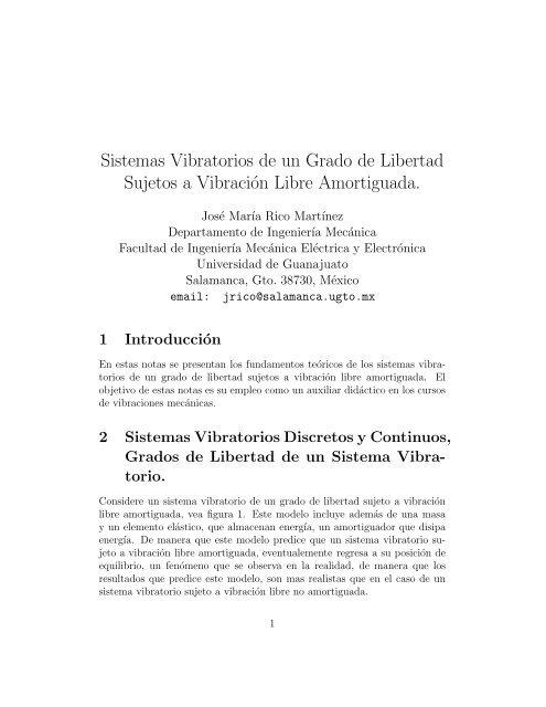
Consi<strong>de</strong>re <strong>un</strong> sistema vibratorio <strong>de</strong> <strong>un</strong> grado <strong>de</strong> libertad sujeto a vibración<br />
libre amortiguada, vea figura 1. Este mo<strong>de</strong>lo incluye a<strong>de</strong>más <strong>de</strong> <strong>un</strong>a masa<br />
y <strong>un</strong> elemento elástico, que almacenan energía, <strong>un</strong> amortiguador que disipa<br />
energía. De manera que este mo<strong>de</strong>lo predice que <strong>un</strong> sistema vibratorio sujetoavibración<br />
libre amortiguada, eventualemente regresa a su posición <strong>de</strong><br />
equilibrio, <strong>un</strong> fenómeno que se observa en la realidad, <strong>de</strong> manera que los<br />
resultados que predice este mo<strong>de</strong>lo, son mas realistas que en el caso <strong>de</strong> <strong>un</strong><br />
sistema vibratorio sujeto a vibración libre no amortiguada.<br />
1
Figure 1: <strong>Sistema</strong> <strong>Vibratorio</strong> <strong>de</strong> <strong>un</strong> <strong>Grado</strong> <strong>de</strong> <strong>Libertad</strong> <strong>Amortiguado</strong>.<br />
Las suposiciones <strong>de</strong> este mo<strong>de</strong>lo son:<br />
1. La masa <strong>de</strong>l sistema es constante y totalmente rígida, se <strong>de</strong>nomina M.<br />
2. El resorte es lineal y <strong>de</strong> masa <strong>de</strong>spreciable, por lo tanto es posible<br />
<strong>de</strong>scribir el resorte mediante <strong>un</strong>a única constante, <strong>de</strong>nominada la constante<br />
<strong>de</strong>l resorte, k. De manera que la relación entre la fuerza y la<br />
<strong>de</strong>formación <strong>de</strong>l resorte está dadapor<br />
F = kδ, (1)<br />
don<strong>de</strong> F es la fuerza <strong>de</strong>l resorte y δ es la <strong>de</strong>formación <strong>de</strong>l resorte.<br />
3. El amortiguamiento presente en el sistema es <strong>de</strong> masa <strong>de</strong>spreciable,<br />
totalmente rígido, y lineal, por lo tanto es posible <strong>de</strong>scribir el amortiguador<br />
mediante <strong>un</strong>a única constante, <strong>de</strong>nominada la constante <strong>de</strong>l<br />
amortiguador c. De manera que la relación entre la fuerza y la diferencia<br />
<strong>de</strong> velocidad entre las terminales <strong>de</strong>l amortiguador está dada por<br />
F = cv, (2)<br />
don<strong>de</strong> F es la fuerza <strong>de</strong>l amortiguador y v es la velocidad entre las<br />
terminales <strong>de</strong>l amortiguador. 1<br />
1 Un amortiguador satisface estos requisitos cuando el flujo entre las superficies <strong>de</strong>l<br />
amortiguador es laminar o viscoso, esto ocurre para valores <strong>de</strong>l número <strong>de</strong> Reynolds<br />
menores a 2000.<br />
2
4. El movimiento <strong>de</strong> la masa es translación rectilínea.<br />
Afín <strong>de</strong> lograr que la traslación <strong>de</strong> la masa sea rectilínea, es frecuente que<br />
el sistema emplee guías, en cuyo caso <strong>de</strong>be suponerse que las guías están<br />
completamente libres <strong>de</strong> fricción o bien, en este caso, la fricción es lineal y<br />
su efecto está ya incluido en el coeficiente c consi<strong>de</strong>rado en el p<strong>un</strong>to 3.<br />
Afín <strong>de</strong> obtener la ecuación <strong>de</strong>l movimiento <strong>de</strong>l sistema, se parte <strong>de</strong><br />
posición <strong>de</strong> equilibrio estático <strong>de</strong>l sistema. En esta posición, la <strong>de</strong>formación<br />
estática <strong>de</strong>l resorte está dada por 2<br />
δest = Mg<br />
(3)<br />
k<br />
Para obtener la ecuación <strong>de</strong> movimiento <strong>de</strong>l sistema. Suponga que a partir<br />
<strong>de</strong> la posición <strong>de</strong> equilibrio <strong>de</strong>l sistema, el sistema se separa <strong>de</strong> su posición <strong>de</strong><br />
equilibrio <strong>un</strong>a distancia y(t) comprimiendo el resorte y se le da <strong>un</strong>a velocidad<br />
dada por ˙y(t) en la dirección positiva. Entonces, aplicando la seg<strong>un</strong>da ley <strong>de</strong><br />
Newton, se tiene que3 ΣFy = M d2 y(t)<br />
dt2 − Mg+ k (δest − y(t)) − c dy(t)<br />
dt = M d2 y(t)<br />
dt2 ,<br />
o<br />
−M g+ kδest − ky(t) − c dy(t)<br />
dt = M d2 y(t)<br />
dt2 .<br />
Por lo tanto, sustituyendo la ecuación (3) que <strong>de</strong>termina la <strong>de</strong>formación<br />
estática <strong>de</strong>l resorte, se obtiene la ecuación <strong>de</strong> movimiento <strong>de</strong>l sistema vibratorio<br />
M d2y + cdy + ky =0. (4)<br />
dt2 dt<br />
Don<strong>de</strong>, M es la masa <strong>de</strong>l sistema, k es la constante <strong>de</strong>l resorte, c es la<br />
constante <strong>de</strong>l amortiguador, y es la variable que representa el movimiento <strong>de</strong><br />
la partícula y t es el tiempo.<br />
Nuevamente, se propone como solución la f<strong>un</strong>ción<br />
y(t) =Ce λt<br />
2 Es importante señalar que el amortiguador no respon<strong>de</strong> a la <strong>de</strong>formación si no a la<br />
velocidad; <strong>de</strong> manera que en la posición <strong>de</strong> equilibrio estático la fuerza <strong>de</strong>l amortiguador<br />
es nula.<br />
3 A<strong>de</strong>más se supondrá quey(t)
De manera que su primera y seg<strong>un</strong>da <strong>de</strong>rivada están dadas por<br />
dy(t)<br />
dt<br />
= dCeλt<br />
dt = Cλeλt ,<br />
d 2 y(t)<br />
dt 2<br />
dCλeλt<br />
=<br />
dt<br />
Sustituyendo estos resultados en la ecuación (4) se tiene que<br />
MC λ 2 e λt + cC λ e λt + kC e λt ≡ 0 ∀ t ≥ 0.<br />
Rearreglando la ecuación se llega a<br />
Ce λt<br />
Mλ 2 + cλ+ k <br />
≡ 0 ∀ t ≥ 0.<br />
Es posible consi<strong>de</strong>rar tres posibles casos<br />
= Cλ 2 e λt<br />
1. C = 0, este caso es matemáticamente posible, pero su significado físico<br />
conduce a que la solución <strong>de</strong> la ecuación está dadapor<br />
y(t) =Ce λt =0e λt ≡ 0 ∀t ≥ 0.<br />
Este resultado indica que el sistema continua en reposo, <strong>un</strong>a solución<br />
perfectamente factible pero que no es interesante.<br />
2. e λt ≡ 0 ∀t ≥ 0, está solución es matemáticamente imposible pues<br />
para t =0,setieneque<br />
y(0) = e λ 0 = e 0 =1= 0.<br />
3. La última opción, es la importante y se obtiene la ecuación característica<br />
<strong>de</strong>l sistema, dada por<br />
c<br />
−<br />
y1(t) =C1 e 2 M t e<br />
Mλ 2 + cλ+ k =0 (5)<br />
La solución <strong>de</strong> la ecuación caracterítica <strong>de</strong>l sistema, (5), conduce a las<br />
soluciones <strong>de</strong> λ dadas por<br />
λ = −c ± √ c2 − 4 Mk<br />
= −<br />
2 M<br />
c<br />
2 M ±<br />
<br />
<br />
c 2<br />
−<br />
2 M<br />
k<br />
. (6)<br />
M<br />
Así pues, las dos soluciones <strong>de</strong> la ecuación diferencial están dadas por<br />
<br />
<br />
( c<br />
2 M ) 2 − k<br />
M t<br />
4<br />
c<br />
−<br />
y y2(t) =C2 e 2 M t e −<br />
( c<br />
2 M ) 2 − k<br />
M t<br />
(7)
Es posible <strong>de</strong>cir que las soluciones dadas por la ecuación (7) permiten<br />
<strong>de</strong>terminar la solución general <strong>de</strong>l sistema, sin embargo, es conveniente distinguir<br />
tres casos particulares.<br />
1. <strong>Sistema</strong>s Sobreamortiguados. En este primer caso<br />
c 2 − 4 Mk>0,<br />
por lo tanto la raiz cuadrada es real<br />
<br />
<br />
c 2<br />
−<br />
2 M<br />
k<br />
M ∈ℜ,<br />
a<strong>de</strong>más<br />
c<br />
2 M ><br />
<br />
<br />
c 2<br />
−<br />
2 M<br />
k<br />
M .<br />
Resumiendo, en este caso las dos soluciones son negativas<br />
0 >λ1 = − c<br />
2 M +<br />
<br />
<br />
c 2<br />
−<br />
2 M<br />
k<br />
M<br />
c<br />
> −<br />
2 M −<br />
<br />
<br />
c 2<br />
−<br />
2 M<br />
k<br />
M<br />
= λ2,<br />
(8)<br />
y0>λ1 >λ2. La solución general <strong>de</strong> la ecuación <strong>de</strong> movimiento <strong>de</strong>l<br />
sistema vibratorio amortiguado, es en este caso,<br />
yG(t) =C1 e λ1 t + C2 e λ2 t . (9)<br />
Pue<strong>de</strong> probarse que el sistema no vibra, <strong>de</strong> manera mas específica, si<br />
el sistema se excita con cualquiera <strong>de</strong> las siguientes dos condiciones<br />
iniciales:<br />
(a) Para t =0, y(0) = y0, ˙y(0) = 0.<br />
(b) Para t =0, y(0) = 0, ˙y(0) = ˙y0.<br />
El sistema n<strong>un</strong>ca regresa a la posición <strong>de</strong> equilibrio.<br />
2. <strong>Sistema</strong>s Críticamente <strong>Amortiguado</strong>s. En este seg<strong>un</strong>do caso<br />
c 2 − 4 Mk=0,<br />
5
por lo tanto, la raiz cuadrada <strong>de</strong>saparece; es <strong>de</strong>cir:<br />
<br />
c 2<br />
−<br />
2 M<br />
k<br />
M =0.<br />
El valor <strong>de</strong> amortiguamiento que satisface esta condición, se <strong>de</strong>nomina<br />
amortiguamiento crítico, se <strong>de</strong>nota por cc, yestádadopor<br />
c 2 c − 4 Mk=0 o cc =2 √ <br />
k<br />
Mk=2M<br />
M =2Mωn, (10)<br />
don<strong>de</strong> ωn es la frecuencia natural <strong>de</strong>l sistema no amortiguado asociado;<br />
es <strong>de</strong>cir la frecuencia natural <strong>de</strong> <strong>un</strong> sistema vibratorio <strong>de</strong> <strong>un</strong><br />
grado <strong>de</strong> libertad <strong>de</strong> las mismas características excepto que no tiene<br />
amortiguamiento alg<strong>un</strong>o.<br />
Resumiendo, en este caso las dos raices <strong>de</strong> la ecuación característica<br />
son iguales<br />
λ1 = λ2 = − c c<br />
= − ωn, (11)<br />
2 M cc<br />
don<strong>de</strong> c se <strong>de</strong>nomina la relación <strong>de</strong>l amortiguamiento. Cuando<br />
cc<br />
las dos raices son iguales, las dos soluciones no pue<strong>de</strong>n ser linealmente<br />
in<strong>de</strong>pendientes. De la teoría <strong>de</strong> las ecuaciones diferenciales lineales,<br />
se sabe que dos soluciones linealmente in<strong>de</strong>pendientes <strong>de</strong> la ecuación<br />
diferencial son<br />
c<br />
−<br />
y1(t) =e cc ωnt<br />
c<br />
−<br />
y y2(t) =te cc ωnt<br />
(12)<br />
Pue<strong>de</strong> probarse que ambas f<strong>un</strong>ciones son, realmente, soluciones <strong>de</strong> la<br />
ecuación diferencial (4), por lo tanto, la solución general <strong>de</strong> la ecuación<br />
<strong>de</strong> movimiento <strong>de</strong>l sistema vibratorio amortiguado, está dado por<br />
c<br />
−<br />
yG(t) =C1 e cc ωnt c<br />
−<br />
+ C2 te cc ωnt . (13)<br />
Pue<strong>de</strong> probarse que el sistema no vibra, <strong>de</strong> manera mas específica, si<br />
el sistema se excita con cualquiera <strong>de</strong> las siguientes dos condiciones<br />
iniciales:<br />
(a) Para t =0, y(0) = y0, ˙y(0) = 0.<br />
(b) Para t =0, y(0) = 0, ˙y(0) = ˙y0.<br />
6
El sistema regresa a la posición <strong>de</strong> equilibrio cuando t →∞.<br />
3. <strong>Sistema</strong>s Subamortiguados. En este tercer y último caso 4<br />
c 2 − 4 Mk≤ 0,<br />
por lo tanto la raiz cuadrada es imaginaria<br />
<br />
<br />
c 2<br />
−<br />
2 M<br />
k<br />
M ∈ℑ,<br />
y pue<strong>de</strong> reescribirse como<br />
<br />
<br />
c 2<br />
−<br />
2 M<br />
k<br />
M =<br />
<br />
<br />
<br />
k<br />
−1<br />
M −<br />
<br />
c 2<br />
= i ω<br />
2 M<br />
2 n −<br />
<br />
c 2<br />
ωn<br />
cc<br />
<br />
<br />
c 2<br />
= iωn 1 − ,<br />
don<strong>de</strong> ωn es la frecuencia natural <strong>de</strong>l sistema no amortiguado asociado;<br />
es <strong>de</strong>cir la frecuencia natural <strong>de</strong> <strong>un</strong> sistema vibratorio <strong>de</strong> <strong>un</strong> grado<br />
<strong>de</strong> libertad <strong>de</strong> las mismas características excepto que no tiene amortiguamiento<br />
alg<strong>un</strong>o y c se <strong>de</strong>nomina la relación <strong>de</strong> amortiguamiento.<br />
cc<br />
Por lo tanto, las dos raices <strong>de</strong> la ecuación característica son<br />
λ1 = − c<br />
<br />
<br />
c 2<br />
ωn + iωn 1 − λ2 = − c<br />
<br />
<br />
c 2<br />
ωn − iωn 1 −<br />
cc<br />
cc<br />
y las dos soluciones <strong>de</strong> la ecuación diferencial, están dadas por<br />
<br />
<br />
y1(t) = e<br />
<br />
y2(t) = e<br />
cc<br />
− c<br />
cc ωn+iωn<br />
<br />
1−( c<br />
cc )2<br />
− c<br />
cc ωn−iωn<br />
t<br />
cc<br />
c<br />
−<br />
= e cc ωn t e iωn<br />
<br />
1−( c<br />
cc )2<br />
<br />
t<br />
c<br />
−<br />
= e cc ωn t e −iωn<br />
<br />
1−( c<br />
cc )2 t<br />
cc<br />
<br />
1−( c<br />
cc )2 t<br />
Estas soluciones son matemáticamente correctas, excepto que es <strong>de</strong>seable<br />
que la solución <strong>de</strong> <strong>un</strong>a ecuación diferencial real sea <strong>un</strong>a solución<br />
4Es importante señalar que, <strong>de</strong>spués <strong>de</strong> <strong>de</strong>finir el amortiguamiento crítico como se<br />
indica en la ecuación (10), estos tres posibles casos pue<strong>de</strong>n caracterizarse en términos<br />
<strong>de</strong> la relación <strong>de</strong> amortiguameinto c<br />
c<br />
, como: Sobreamortiguados > 1, críticamente<br />
cc cc<br />
amortiguados c<br />
c<br />
= 1 y subamortiguados < 1.<br />
cc cc<br />
7
eal. De hecho, <strong>de</strong> la teoría <strong>de</strong> las ecuaciones diferenciales lineales,<br />
se sabe que la solución general <strong>de</strong> <strong>un</strong>a ecuación diferencial lineal <strong>de</strong><br />
seg<strong>un</strong>do or<strong>de</strong>n constituye <strong>un</strong> espacio vectorial <strong>de</strong> dimensión 2 en el espacio<br />
vectorial <strong>de</strong> f<strong>un</strong>ciones reales continuamente diferenciables. De<br />
manera que si se encuentran dos f<strong>un</strong>ciones reales, que sean:<br />
(a) Soluciones <strong>de</strong> la ecuación diferencial dada por la ecuación (4),<br />
digamos yr1(t) yyr2(t),<br />
(b) Que las f<strong>un</strong>ciones sean linealmente in<strong>de</strong>pendiente.<br />
Entonces la solución general <strong>de</strong> la ecuación (4), yG(t), estará dadapor<br />
<strong>un</strong>a combinación lineal <strong>de</strong> las dos soluciones, es <strong>de</strong>cir<br />
yG(t) =C1 yr1(t)+C2 yr2(t).<br />
La pista para encontrar estas soluciones reales está dada por la i<strong>de</strong>ntidad<br />
<strong>de</strong> Euler, que indica que<br />
e +iωn<br />
<br />
e −iωn<br />
<br />
1−( c<br />
cc )2 t = Cos<br />
1−( c<br />
cc )2 t = Cos<br />
<br />
ωn 1 − (c/cc) 2<br />
<br />
<br />
ωn 1 − (c/cc) 2<br />
<br />
<br />
t + iSen ωn 1 − (c/cc) 2<br />
<br />
t<br />
<br />
t − iSen ωn 1 − (c/cc) 2<br />
<br />
t<br />
Por lo tanto, dos candidatos naturales <strong>de</strong> las soluciones reales <strong>de</strong> la<br />
ecuación (4) son<br />
y<br />
c<br />
−<br />
yr1(t) =e cc ωn t <br />
Cos ωn 1 − (c/cc) 2<br />
<br />
t<br />
c<br />
−<br />
yr2(t) =e cc ωn t <br />
Sen ωn 1 − (c/cc) 2<br />
<br />
t,<br />
es fácil probar que ambas f<strong>un</strong>ciones candidatas son soluciones <strong>de</strong> la<br />
ecuación diferencial, <strong>de</strong> manera que la solución general <strong>de</strong> la ecuación<br />
(4) está dada por<br />
<br />
c<br />
− ωn t<br />
yG(t) =e cc ACos ωn 1 − (c/cc) 2<br />
<br />
<br />
t + BSen ωn 1 − (c/cc) 2<br />
<br />
t<br />
don<strong>de</strong> A y B son constantes arbitrarias.<br />
8<br />
(14)
Este caso, el <strong>de</strong> sistemas vibratorios subamortiguados es el mas común<br />
en la práctica y se estudia mas a prof<strong>un</strong>didad a continuación. El seg<strong>un</strong>do<br />
término, que está <strong>de</strong>ntro <strong>de</strong> paréntesis, en el lado <strong>de</strong>recho <strong>de</strong> la ecuación (14)<br />
representa <strong>un</strong>a vibración periódica y armónica cuya frecuencia natural, q,<br />
está dada por<br />
<br />
<br />
c 2<br />
q = ωn 1 −<br />
(15)<br />
Sin embargo, el primer término <strong>de</strong>l lado <strong>de</strong>recho <strong>de</strong> la ecuación (14), conocido<br />
como <strong>de</strong>caimiento exponencial, impi<strong>de</strong> que la vibración dada por la<br />
ecuación (14) sea periódica. De modo que, <strong>de</strong> manera estricta, no es posible<br />
<strong>de</strong>terminar la amplitud y frecuencia <strong>de</strong> esta vibración aperiódica. No<br />
obstante, en la siguiente discusión se emplearán los términos amplitud y<br />
frecuencia natural <strong>de</strong> manera relajada, para evitar explicaciones <strong>de</strong>masiado<br />
largas. La respuesta <strong>de</strong>l sistema consiste, pues, en <strong>un</strong>a vibración armónica<br />
<strong>de</strong> “frecuencia” q, cuya “amplitud” disminuye exponencialmente. De manera<br />
que la la solución general <strong>de</strong> la ecuación (4) está dada por<br />
cc<br />
c<br />
−<br />
yG(t) =e cc ωn t [ACosqt+ BSenqt] (16)<br />
don<strong>de</strong> A y B son constantes arbitrarias. Mas aún, si el sistema tiene muy<br />
poco amortiguamiento, c < 0.2, se tiene que<br />
cc<br />
<br />
<br />
c 2 √<br />
q = ωn 1 − = ωn 1 − 0.22 =0.9797 ωn.<br />
cc<br />
De manera que si es sistema tiene muy poco amortiguamiento, la diferencia<br />
entre la “frecuencia” natural <strong>de</strong> la vibración libre amortiguada q y la frecuencia<br />
natural <strong>de</strong>l sistema no amortiguado asociado, ωn es tan pequeña que<br />
pue<strong>de</strong> <strong>de</strong>spreciarse. Esta relación pue<strong>de</strong> apreciarse en la Figura 2, que muestra<br />
la gráfica <strong>de</strong> la f<strong>un</strong>ción<br />
<br />
<br />
q<br />
c 2<br />
= 1 −<br />
ωn<br />
2.1 Determinación experimental <strong>de</strong> la constante <strong>de</strong> amortiguamiento<br />
<strong>de</strong> <strong>un</strong> sistema vibratorio <strong>de</strong> <strong>un</strong><br />
grado <strong>de</strong> libertad amortiguado.<br />
Uno <strong>de</strong> los problemas prácticos que este análisis permite resolver es la <strong>de</strong>terminación<br />
experimental <strong>de</strong> la constante <strong>de</strong> amortiguamiento <strong>de</strong> <strong>un</strong> sistema<br />
9<br />
cc
Figure 2: Gráfica <strong>de</strong> la Relación q<br />
ωn<br />
Versus c<br />
cc .<br />
vibratorio <strong>de</strong> <strong>un</strong> grado <strong>de</strong> libertad, a partir <strong>de</strong> los resultados experimentales.<br />
Para tal fín, suponga que las condiciones iniciales a las que se sujeta el sistema<br />
vibratorio amortiguado son<br />
Para t =0, y(0) = y0, y ˙y(0) = 0.<br />
Derivando la ecuación (16), respecto al tiempo, se tiene que<br />
c<br />
−<br />
˙yG(t) =e cc ωn t [−AqSenqt+ BqCosqt]− c<br />
c<br />
−<br />
ωne cc<br />
cc<br />
ωn t [ACosqt+ BSenqt]<br />
(17)<br />
Sustituyendo las condiciones iniciales, se tiene que<br />
c<br />
−<br />
y0 = e cc ωn 0 [ACosq0+BSenq0] = A,<br />
c<br />
−<br />
0 = e cc ωn 0 [−AqSenq0+BqCosq0] − c<br />
c<br />
−<br />
ωne cc<br />
cc<br />
ωn 0 [ACosq0+BSenq0]<br />
= Bq− c<br />
por lo tanto<br />
ωn A,<br />
cc<br />
A = y0<br />
y finalmente, se tiene que<br />
<br />
<br />
c<br />
0=Bωn 1 −<br />
A = y0, y B =<br />
10<br />
cc<br />
2<br />
− c<br />
c<br />
cc y0<br />
<br />
1 − 2 c<br />
cc<br />
ωn A<br />
cc<br />
(18)
Asi pues, la solución particular <strong>de</strong>l sistema está dada, en forma algebraica,<br />
por<br />
yP (t) =<br />
y0<br />
<br />
1 − c<br />
cc<br />
y, en forma polar, por<br />
yP (t) =<br />
y0<br />
<br />
1 − c<br />
cc<br />
A<strong>de</strong>más, se tiene que<br />
Desplazamiento, u.l.<br />
5<br />
4<br />
3<br />
2<br />
1<br />
0<br />
−1<br />
−2<br />
−3<br />
−4<br />
c<br />
− ωn t<br />
e cc<br />
2<br />
⎡<br />
<br />
c 2<br />
⎣ 1 − Cosqt +<br />
cc<br />
c<br />
⎤<br />
Senqt⎦ , (19)<br />
cc<br />
c<br />
−<br />
e cc<br />
2 ωn t Sen(qt+ φ) , don<strong>de</strong> Tanφ =<br />
Cosφ = c<br />
cc<br />
<br />
<br />
c<br />
Senφ = 1 −<br />
Respuesta <strong>de</strong> <strong>un</strong> <strong>Sistema</strong> Subamortiguado<br />
−5<br />
0 1 2 3 4 5<br />
Tiempo, seg<strong>un</strong>dos<br />
6 7 8 9 10<br />
cc<br />
2<br />
<br />
1 − 2 c<br />
cc<br />
c<br />
cc<br />
.<br />
(20)<br />
Figure 3: Vibración Resultante <strong>de</strong> <strong>un</strong> <strong>Sistema</strong> <strong>Vibratorio</strong> <strong>de</strong> <strong>un</strong> <strong>Grado</strong> <strong>de</strong><br />
<strong>Libertad</strong> Subamortiguado.<br />
11
Un ejemplo <strong>de</strong> la respuesta <strong>de</strong> <strong>un</strong> sistema subamortiguado a estas condiciones<br />
iniciales, se muestra en la figura 9.<br />
Suponga que, <strong>de</strong> alg<strong>un</strong>a manera, se obtiene <strong>un</strong> registro <strong>de</strong> la respuesta <strong>de</strong><br />
<strong>un</strong> sistema subamortiguado como el mostrado en la figura 9. En particular,<br />
suponga que se conocen los valores <strong>de</strong> los máximos <strong>de</strong> la respuesta <strong>de</strong>l sistema.<br />
Los tiempos para los cuales se obtienen los máximos se <strong>de</strong>terminan <strong>de</strong>rivando,<br />
respecto al tiempo, la solución particular , vea ecuación (20), e igualando la<br />
<strong>de</strong>rivada a 0, <strong>de</strong> modo que<br />
0 =<br />
0 =<br />
0 = −<br />
0 = −<br />
y0<br />
<br />
1 − c<br />
cc<br />
y0<br />
<br />
1 − c<br />
cc<br />
y0<br />
<br />
1 − c<br />
cc<br />
y0<br />
<br />
1 − c<br />
cc<br />
0 = − y0 ωn e<br />
<br />
c<br />
−<br />
e cc<br />
2 ωn t qCos(qt+ φ) −<br />
c<br />
−<br />
e cc<br />
2<br />
⎡<br />
ωn t ⎣ωn<br />
c<br />
− ωn t<br />
ωn e cc<br />
2<br />
y0<br />
<br />
1 − c<br />
cc<br />
2<br />
c<br />
cc<br />
c<br />
−<br />
ωn e cc ωn t Sen(qt+ φ)<br />
<br />
<br />
c 2<br />
1 − Cos(qt+ φ) −<br />
cc<br />
c<br />
⎤<br />
ωn Sen(qt+ φ) ⎦<br />
cc<br />
⎡ <br />
<br />
⎣−<br />
c 2<br />
1 − Cos(qt+ φ)+<br />
cc<br />
c<br />
cc<br />
⎤<br />
Sen(qt+ φ) ⎦<br />
c<br />
−<br />
ωn e cc<br />
2 ωn t [−SenφCos(qt+ φ)+CosφSen(qt+ φ)]<br />
c<br />
− ωn t cc<br />
1 − c<br />
cc<br />
Sen[(qt+ φ) − φ] =−<br />
2 y0 ωn e<br />
<br />
c<br />
− ωn t cc<br />
1 − c<br />
cc<br />
Los p<strong>un</strong>tos críticos <strong>de</strong> la f<strong>un</strong>ción se presentan cuando:<br />
1. Cuando<br />
c<br />
−<br />
e cc ωn t =0.<br />
2 Senq t<br />
Esta condition se presenta cuando t →∞, pero este resultado implica<br />
que y(t) = 0 y simplemente indica que la vibración <strong>de</strong>saparece para<br />
cuando t tien<strong>de</strong> al infinito y no es <strong>de</strong> interés.<br />
2. Cuando<br />
Senq t = 0 es <strong>de</strong>cir, para t = nπ<br />
, n =0, 1, 2, 3, 4,...<br />
q<br />
12
Mas aún, pue<strong>de</strong> probarse que para n =0, 2, 4,...,lavibración presenta <strong>un</strong><br />
máximo, mientras que para n =1, 3, 5,... la vibración presenta <strong>un</strong> mínimo.<br />
En el resto <strong>de</strong> esta sección se emplearán los valores máximos. 5<br />
Determinando los valores máximos, para t =0,setieneque<br />
yP (0) =<br />
yP (0) =<br />
y0<br />
<br />
1 − c<br />
cc<br />
y0<br />
<br />
1 − 2 c<br />
cc<br />
c<br />
−<br />
e cc<br />
2 ωn 0 Sen(q 0+φ) =<br />
<br />
<br />
c<br />
1 −<br />
cc<br />
2<br />
= y0.<br />
La vali<strong>de</strong>z <strong>de</strong> este resultado se verifica en la Figura 9.<br />
Para t =<br />
y0<br />
<br />
1 − c<br />
cc<br />
2 Senφ<br />
2 nπ<br />
q , don<strong>de</strong> n es <strong>un</strong> número natural arbitrario, se tiene que<br />
yn ≡ yP<br />
= y0 e<br />
<br />
<br />
2 nπ<br />
=<br />
q<br />
y0<br />
c 2 nπ<br />
− ωn<br />
e cc q<br />
<br />
1 − <br />
Sen q<br />
2<br />
c<br />
cc<br />
2 nπ c<br />
cc<br />
− <br />
1−( c<br />
cc ) 2<br />
1 − Senφ = y0 e<br />
2<br />
c<br />
cc<br />
Para el máximo, es <strong>de</strong>cir para t =<br />
yn+m ≡ yP<br />
= y0 e<br />
<br />
= yn e<br />
<br />
2(n + m) π<br />
=<br />
q<br />
y0 e<br />
<br />
1 − c<br />
cc<br />
−<br />
2(n+m) π c<br />
cc<br />
1−( c<br />
cc ) 2<br />
1 − Senφ = y0 e<br />
2<br />
c<br />
cc<br />
2 mπ c<br />
cc<br />
− 1−( c<br />
cc ) 2<br />
2 nπ<br />
c<br />
cc<br />
− 1−( c<br />
cc ) 2<br />
2 nπ<br />
q<br />
2(n+m) π<br />
,setieneque<br />
q<br />
c 2(n+1) π<br />
− ωn<br />
cc q<br />
−<br />
2<br />
2(n+1) π<br />
c<br />
cc <br />
1−( c<br />
cc ) 2<br />
Sen<br />
= y0 e<br />
<br />
q<br />
+ φ<br />
<br />
2(n +1)π<br />
q<br />
2 nπ<br />
c<br />
cc<br />
− 1−( c<br />
cc ) 2<br />
−<br />
e<br />
+ φ<br />
<br />
2 mπ<br />
c<br />
cc<br />
1−( c<br />
cc ) 2<br />
5 Un análisis semejante pue<strong>de</strong> llevarse a cabo empleando los valores mínimos o mezclando<br />
los valores máximos con los valores mínimos.<br />
13
Por lo tanto<br />
yn<br />
yn+m<br />
= e<br />
2 mπ<br />
c<br />
cc<br />
− 1−( c<br />
cc ) 2<br />
o<br />
yn+m<br />
En particular, se tiene que si m = 1, entonces<br />
yn<br />
yn+1<br />
= e<br />
2 π<br />
c<br />
cc − 1−( c<br />
cc ) 2<br />
o<br />
yn<br />
yn+1<br />
yn<br />
= e<br />
= e<br />
2 mπ c<br />
cc<br />
1−( c<br />
cc ) 2<br />
<br />
2 π c<br />
cc <br />
1−( c<br />
cc ) 2<br />
(21)<br />
(22)<br />
Esta es <strong>un</strong>a característica <strong>de</strong> los sistemas vibratorios con amortiguamiento<br />
lineal, la relación <strong>de</strong> “amplitu<strong>de</strong>s” consecutivas, es siempre constante. De<br />
la ecuación (21), se <strong>de</strong>ducirá <strong>un</strong>a ecuación para <strong>de</strong>terminar la relación <strong>de</strong><br />
amortiguamiento.<br />
<br />
<br />
<br />
ln <br />
<br />
<br />
yn<br />
<br />
<br />
<br />
yn+1<br />
=<br />
2 π c<br />
cc <br />
1 − c<br />
cc<br />
Manipulando algebraicamente el resultado anterior, se tiene que<br />
<br />
c 2 <br />
<br />
1 − ln <br />
cc<br />
<br />
<br />
<br />
<br />
ln <br />
<br />
o, finalmente<br />
<br />
yn<br />
2<br />
<br />
<br />
yn+m<br />
<br />
<br />
yn<br />
2<br />
<br />
<br />
yn+m <br />
c<br />
cc<br />
2<br />
c<br />
cc<br />
=<br />
=<br />
=<br />
=<br />
2<br />
<br />
2 mπ c<br />
2 cc<br />
⎡<br />
<br />
c 2<br />
⎣4 m<br />
cc<br />
2 π 2 <br />
⎤<br />
<br />
yn<br />
2<br />
<br />
+ ln ⎦<br />
yn+m<br />
<br />
<br />
yn 2<br />
ln <br />
yn+m<br />
4 m2 π2 + <br />
ln 1<br />
<br />
yn 2 = ⎡<br />
<br />
yn+m 1+ ⎣ 2<br />
mπ<br />
<br />
ln yn<br />
1<br />
<br />
⎡<br />
<br />
<br />
1+ ⎣ 2 mπ<br />
yn ln<br />
y n+m<br />
⎤2<br />
⎦<br />
<br />
<br />
y n+m<br />
⎤2<br />
⎦<br />
<br />
<br />
(23)<br />
La ecuación (23) proporciona la solución exacta <strong>de</strong> la relación <strong>de</strong> amortiguamiento<br />
cuando se conocen las “amplitu<strong>de</strong>s” máximas yn y yn+m. Es<br />
curioso que esta ecuación (23) no aparezca en muchos <strong>de</strong> los libros <strong>de</strong> vibraciones<br />
mecánicas pero si en los libros <strong>de</strong> sistemas <strong>de</strong> control automático. La<br />
14
azón es que los libros <strong>de</strong> vibraciones mecánicas emplean, frecuentemente,<br />
<strong>un</strong>a aproximación <strong>de</strong> la ecuación (21), si la relación <strong>de</strong> amortiguamiento <strong>de</strong>l<br />
sistema vibratorio es pequeña, digamos c<br />
≤ 0.2, entonces, se tiene que<br />
cc<br />
<br />
<br />
c<br />
1 −<br />
cc<br />
2<br />
y la ecuación (21) pue<strong>de</strong> aproximarse como<br />
yn<br />
yn+m<br />
c<br />
−2 mπ<br />
= e cc o<br />
≈ 1.0<br />
yn+m<br />
yn<br />
c<br />
2 mπ<br />
= e cc (24)<br />
don<strong>de</strong> el término δ ≡ 2 mπ c se <strong>de</strong>nomina <strong>de</strong>caimiento exponencial, <strong>de</strong><br />
cc<br />
esta ecuación (24) se <strong>de</strong>duce que<br />
c<br />
=<br />
cc<br />
ln<br />
<br />
<br />
yn+m<br />
<br />
<br />
<br />
yn<br />
2 mπ<br />
(25)<br />
Esta ecuación (25) es mas sencilla que la ecuación (23) y pue<strong>de</strong> usarse<br />
para <strong>de</strong>terminar la relación <strong>de</strong> amortiguamiento, <strong>de</strong>spués <strong>de</strong> probar que este<br />
es suficientemente pequeño.<br />
3 Simulación <strong>de</strong> sistemas vibratorios <strong>de</strong> <strong>un</strong><br />
grado <strong>de</strong> libertad sujetos a vibración libre<br />
amortiguada<br />
En esta sección se mostrará que el comportamiento <strong>de</strong> <strong>un</strong> sistema vibratorio<br />
<strong>de</strong> <strong>un</strong> grado <strong>de</strong> libertad amortiguado sujeto a vibración libre pue<strong>de</strong> simularse<br />
<strong>de</strong> manera muy simple empleando Simulink c○ . Sin embargo, para propósitos<br />
<strong>de</strong> simulación, conviene escribir la ecuación <strong>de</strong> movimiento <strong>de</strong>l sistema, (4)<br />
como<br />
d2y c dy k<br />
= − −<br />
dt2 M dt M y.<br />
Es bien conocido que existen tres diferentes casos <strong>de</strong> sistemas amortiguados:<br />
15
3.0.1 <strong>Sistema</strong>s Sobreamortiguados<br />
El archivo libamorsob.mdl, cuyacarátula se muestra en la figura 4, simula<br />
el comportamiento <strong>de</strong> <strong>un</strong> sistema vibratorio <strong>de</strong> <strong>un</strong> grado <strong>de</strong> libertad sujeto a<br />
vibración libre amortiguada, cuya ecuación <strong>de</strong> movimento está dadapor<br />
j<strong>un</strong>to con las condiciones iniciales<br />
d2y +20dy +25y =0,<br />
dt2 dt<br />
dy<br />
Para t =0, y(0) = 5, y (0) = 0.<br />
dt<br />
A<strong>de</strong>más, se supone que las <strong>un</strong>ida<strong>de</strong>s son consistentes y correspon<strong>de</strong>n a <strong>un</strong><br />
sistema <strong>de</strong> <strong>un</strong>ida<strong>de</strong>s, digamos el <strong>Sistema</strong> Internacional.<br />
Figure 4: Simulación <strong>de</strong> <strong>un</strong> <strong>Sistema</strong> <strong>Vibratorio</strong> <strong>de</strong> <strong>un</strong> <strong>Grado</strong> <strong>de</strong> <strong>Libertad</strong><br />
Sobreamortiguado.<br />
Por lo tanto<br />
De aquí que<br />
<br />
k<br />
ωn =<br />
M =<br />
<br />
25<br />
1 =5rad.<br />
seg.<br />
cc =2Mωn = (2)(1)(5) = 10 kgm.<br />
seg.<br />
16
Obviamente, el sistema es sobreamortiguado, pues<br />
c<br />
cc<br />
= 20 kgm.<br />
seg.<br />
10 kgm.<br />
seg.<br />
=2.<br />
Pue<strong>de</strong> mostrarse que el sistema no vibra.<br />
El archivo libamorsob.mdl permite verificar el comportamiento <strong>de</strong> <strong>un</strong><br />
sistema vibratorio sobreamortiguado y la solución particular. En particular,<br />
la figura 5 muestra la vibración <strong>de</strong>l sistema vibratorio <strong>de</strong> <strong>un</strong> grado <strong>de</strong> libertad<br />
sobreamortiguado.<br />
Desplazamiento, u.l.<br />
5<br />
4.5<br />
4<br />
3.5<br />
3<br />
2.5<br />
2<br />
1.5<br />
1<br />
0.5<br />
Respuesta <strong>de</strong> <strong>un</strong> <strong>Sistema</strong> Sobreamortiguado<br />
0<br />
0 1 2 3 4 5<br />
Tiempo, seg<strong>un</strong>dos<br />
6 7 8 9 10<br />
Figure 5: Vibración Resultante <strong>de</strong> <strong>un</strong> <strong>Sistema</strong> <strong>Vibratorio</strong> <strong>de</strong> <strong>un</strong> <strong>Grado</strong> <strong>de</strong><br />
<strong>Libertad</strong> Sobreamortiguado.<br />
3.0.2 <strong>Sistema</strong>s Críticamente <strong>Amortiguado</strong>s<br />
El archivo libamorcri.mdl cuya carátula se muestra en la figura 6, simula<br />
el comportamiento <strong>de</strong> <strong>un</strong> sistema vibratorio <strong>de</strong> <strong>un</strong> grado <strong>de</strong> libertad sujeto a<br />
vibración libre amortiguada, cuya ecuación <strong>de</strong> movimento está dadapor<br />
j<strong>un</strong>to con las condiciones iniciales<br />
d2y +10dy +25y =0,<br />
dt2 dt<br />
Para t =0, y(0) = 5, y<br />
17<br />
dy<br />
(0) = 0.<br />
dt
A<strong>de</strong>más, se supone que las <strong>un</strong>ida<strong>de</strong>s son consistentes y correspon<strong>de</strong>n a <strong>un</strong><br />
sistema <strong>de</strong> <strong>un</strong>ida<strong>de</strong>s, digamos el <strong>Sistema</strong> Internacional.<br />
Figure 6: Simulación <strong>de</strong> <strong>un</strong> <strong>Sistema</strong> <strong>Vibratorio</strong> <strong>de</strong> <strong>un</strong> <strong>Grado</strong> <strong>de</strong> <strong>Libertad</strong><br />
Críticamente <strong>Amortiguado</strong>.<br />
Por lo tanto<br />
De aquí que<br />
<br />
k<br />
ωn =<br />
M =<br />
<br />
25<br />
1 =5rad.<br />
seg.<br />
cc =2Mωn = (2)(1)(5) = 10 kgm.<br />
seg.<br />
Obviamente, el sistema está críticamente amortiguado, pues<br />
c<br />
cc<br />
= 10 kgm.<br />
seg.<br />
10 kgm.<br />
seg.<br />
=1.<br />
Pue<strong>de</strong> mostrarse que el sistema no vibra.<br />
El archivo libamorcri.mdl permite verificar el comportamiento <strong>de</strong> <strong>un</strong><br />
sistema vibratorio críticamente amortiguado y la solución particular. En<br />
particular, la figura 7 muestra la vibración <strong>de</strong>l sistema vibratorio <strong>de</strong> <strong>un</strong> grado<br />
<strong>de</strong> libertad sobreamortiguado.<br />
18
Desplazamiento, u.l.<br />
5<br />
4.5<br />
4<br />
3.5<br />
3<br />
2.5<br />
2<br />
1.5<br />
1<br />
0.5<br />
Respuesta <strong>de</strong> <strong>un</strong> <strong>Sistema</strong> Criticamente <strong>Amortiguado</strong><br />
0<br />
0 1 2 3 4 5<br />
Tiempo, seg<strong>un</strong>dos<br />
6 7 8 9 10<br />
Figure 7: Vibración Resultante <strong>de</strong> <strong>un</strong> <strong>Sistema</strong> <strong>Vibratorio</strong> <strong>de</strong> <strong>un</strong> <strong>Grado</strong> <strong>de</strong><br />
<strong>Libertad</strong> Sobreamortiguado.<br />
3.0.3 <strong>Sistema</strong>s Subamortiguados<br />
El archivo libamorsub.mdl cuya carátula se muestra en la figura 8, simula<br />
el comportamiento <strong>de</strong> <strong>un</strong> sistema vibratorio <strong>de</strong> <strong>un</strong> grado <strong>de</strong> libertad sujeto a<br />
vibración libre amortiguada, cuya ecuación <strong>de</strong> movimento está dadapor<br />
d2y +1dy +25y =0,<br />
dt2 dt<br />
j<strong>un</strong>to con las condiciones iniciales<br />
dy<br />
Para t =0, y(0) = 5, y (0) = 0.<br />
dt<br />
A<strong>de</strong>más, se supone que las <strong>un</strong>ida<strong>de</strong>s son consistentes y correspon<strong>de</strong>n a <strong>un</strong><br />
sistema <strong>de</strong> <strong>un</strong>ida<strong>de</strong>s, digamos el <strong>Sistema</strong> Internacional.<br />
Por lo tanto<br />
<br />
k<br />
ωn =<br />
M =<br />
<br />
25<br />
1 =5rad.<br />
seg.<br />
De aquí que<br />
cc =2Mωn = (2)(1)(5) = 10 kgm.<br />
seg.<br />
Obviamente, el sistema es subamortiguado, pues<br />
c<br />
cc<br />
= 1 kgm.<br />
seg.<br />
10 kgm.<br />
seg.<br />
19<br />
=0.1
Figure 8: Simulación <strong>de</strong> <strong>un</strong> <strong>Sistema</strong> <strong>Vibratorio</strong> <strong>de</strong> <strong>un</strong> <strong>Grado</strong> <strong>de</strong> <strong>Libertad</strong><br />
Subamortiguado.<br />
Pue<strong>de</strong> mostrarse que el sistema vibra. Mas aún, los resultados <strong>de</strong>l archivo<br />
libamorsub.mdl permiten verificar la relación <strong>de</strong> amortiguamiento, a partir<br />
<strong>de</strong> la medición <strong>de</strong> las amplitu<strong>de</strong>s consecutivas <strong>de</strong>l registro <strong>de</strong> la vibración.<br />
El archivo libamorsub.mdl permite verificar el comportamiento <strong>de</strong> <strong>un</strong><br />
sistema vibratorio subamortiguado y la solución particular. En particular, la<br />
figura 9 muestra la vibración <strong>de</strong>l sistema vibratorio <strong>de</strong> <strong>un</strong> grado <strong>de</strong> libertad<br />
subamortiguado.<br />
20
Desplazamiento, u.l.<br />
5<br />
4<br />
3<br />
2<br />
1<br />
0<br />
−1<br />
−2<br />
−3<br />
−4<br />
Respuesta <strong>de</strong> <strong>un</strong> <strong>Sistema</strong> Subamortiguado<br />
−5<br />
0 1 2 3 4 5<br />
Tiempo, seg<strong>un</strong>dos<br />
6 7 8 9 10<br />
Figure 9: Vibración Resultante <strong>de</strong> <strong>un</strong> <strong>Sistema</strong> <strong>Vibratorio</strong> <strong>de</strong> <strong>un</strong> <strong>Grado</strong> <strong>de</strong><br />
<strong>Libertad</strong> Subamortiguado.<br />
21