Etude de la couronne solaire en 3D et de son évolution avec SOHO ...

tel-00089354, version 1 - 17 Aug 2006
846 ASCHWANDEN ET AL. Vol. 515
NS distance [deg]
-0.04
-0.06
-0.08
-0.10
-0.12
B(x,t 1)
θ=-10 0
Previous day
10 0 20 0 90 0
-0.04
-0.06
-0.08
-0.10
-0.12
Reference day
(x 1,y 1)
(x n,y n)
-0.14
-0.14
-0.14 -0.12 -0.10 -0.08 -0.06 -0.04 -0.06 -0.04 -0.02 0.00 0.02
EW distance [deg]
EW distance [deg]
Stripe aligned with projection θ=10 0
B(x+Δx,t 2)
-0.04
-0.06
-0.08
-0.10
-0.12
Following day
θ=90 0 20 0 10 0
-10 0
-0.14
-0.00 0.02 0.04 0.06 0.08 0.10
EW distance [deg]
Stripe aligned with projection θ=20 0
Stripe aligned with observed projection Stripe aligned with projection θ=20 0
Stripe aligned with projection θ=30 0
Stripe aligned with projection θ=10 0
Stripe aligned with projection θ=30 0
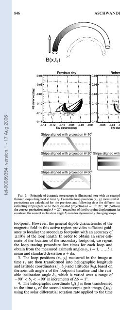
FIG. 3.ÈPrinciple of dynamic stereoscopy is illustrated here with an example of two adjacent loops, where a thicker loop is bright at time t , whereas a
thinner loop is brightest at time t . From the loop positions (x, y ) measured at an intermediate reference time t, i.e., t \ t \ t (middle panel in
1
middle row),
projections are calculated for the
2
previous and following days
i
for
i
di†erent inclination angles Ë of the loop plane (left
1
and right
2
panel in middle row). By
extracting stripes parallel to the calculated projections Ë \ 10¡, 20¡, 30¡ (bottom) it can be seen that both loops appear only co-aligned with the stripe axis for
the correct projection angle Ë \ 20¡, regardless of the footpoint displacement *x between the two loops. The co-alignment criterion can therefore be used to
constrain the correct inclination angle Ë, even for dynamically changing loops.
footpoint. However, the general dipole characteristic of the
magnetic Ðeld in this active region provides sufficient guidance
to localize the secondary footpoint with an accuracy of
[10% of the loop length. In order to obtain an error estimate
of the location of the secondary footpoint, we repeat
the loop tracing procedure Ðve times for each loop and
obtain from the measured azimuth angles a , j \ 1, ..., 5 a
mean and standard deviation a ^ da.
j
3. The loop positions (x , y ) measured in the image at
i i
time t are then transformed into heliographic longitude
1
and latitude coordinates (l , b ) and altitudes (h), based on
ij ij ij
the azimuth angle a of the footpoint baseline and the variable
inclination angle Ë , which is varied over a range of
j
[90¡ \ Ë \ ]90¡ in increments of *Ë \ 1¡.
j
4. The heliographic coordinate l (t ) is then transformed
ij 1
to the time t of the second stereoscopic pair image, l@ (t ),
2
ij 2
using the solar di†erential rotation rate applied to the time
interval (t [ t ). We use the di†erential rotation rate speci-
Ðed by Allen
2
(1973),
1
l@(t ) \ l(t ) ] [13¡.45[ 3¡ sin2 b]
2 1 (t 2 [ t 1 )
. (2)
1 day
The heliographic latitude b and altitude h are assumed to
be constant during the considered
ij
time interval.
ij
5. In the stereoscopic pair image at time t we calculate
the image coordinates (x@ , y@ ) of the projected
2
loop strucij
ij
ture. Parallel to these loop curves (with typical lengths of
n \ 50È200 pixels) we extract image stripes of some width
s
(n w \ 16
pixels) by interpolating the image brightness
F(x, y) at the positions of the curved coordinate grid.
6. The stretched two-dimensional image stripes (n ] n
s w
pixels) are then scanned for parallel brightness ridges,
caused by ““ dynamic ÏÏ structures that are co-aligned (or
parallel-displaced) to the loop projection in image t (for
2