

Etude de la couronne solaire en 3D et de son évolution avec SOHO ...
Etude de la couronne solaire en 3D et de son évolution avec SOHO ...
Etude de la couronne solaire en 3D et de son évolution avec SOHO ...

Create successful ePaper yourself
Turn your PDF publications into a flip-book with our unique Google optimized e-Paper software.
tel-00089354, version 1 - 17 Aug 2006<br />
No. 2, 1999 THREE-DIMENSIONAL ANALYSIS OF SOLAR ACTIVE REGIONS 865<br />
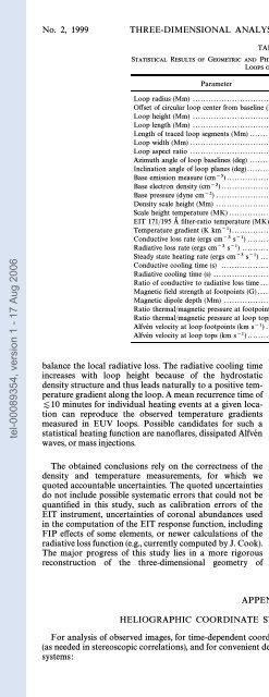
TABLE 4<br />
STATISTICAL RESULTS OF GEOMETRIC AND PHYSICAL PARAMETERS OF THE ANALYZED 30 EUV<br />
LOOPS OF AR 7986<br />
Param<strong>et</strong>er Value<br />
Loop radius (Mm) ......................................... R 0 \ 93 ^ 23<br />
O†s<strong>et</strong> of circu<strong>la</strong>r loop c<strong>en</strong>ter from baseline (Mm) ...... Z 0 \ 62 ^ 27<br />
Loop height (Mm) ......................................... h \ 128 ^ 56<br />
Loop l<strong>en</strong>gth (Mm) ......................................... L \ 433 ^ 136<br />
L<strong>en</strong>gth of traced loop segm<strong>en</strong>ts (Mm) ................... L 1 \ 89 ^ 29<br />
Loop width (Mm) .......................................... w \ 7.1 ^ 0.8<br />
Loop aspect ratio .......................................... L /w \ 61 ^ 20<br />
Azimuth angle of loop baselines (<strong>de</strong>g) ................... a \ 3 ^ 10<br />
Inclination angle of loop p<strong>la</strong>nes (<strong>de</strong>g) .................... Ë \ 7 ^ 37<br />
Base emission measure (cm~5)............................ EM 0 \ 1027.61B0.61<br />
Base electron <strong>de</strong>nsity (cm~3).............................. n e0 \ (1.92 ^ 0.56) ] 109<br />
Base pressure (dyne cm~2) ................................ p 0 \ 0.61 ^ 0.17<br />
D<strong>en</strong>sity scale height (Mm) ................................ j \ 55 ^ 10<br />
Scale height temperature (MK) ........................... T e j \ 1.22 ^ 0.23<br />
EIT 171/195 A Ðlter-ratio temperature (MK) ........... T e EIT \ 1.21 ^ 0.06<br />
Temperature gradi<strong>en</strong>t (K km~1).......................... dT /ds \ 0.96 ^ 4.26<br />
Conductive loss rate (ergs cm~3 s~1) .................... +F C \ ([0.003 ^ 0.005) ] 10~3<br />
Radiative loss rate (ergs cm~3 s~1) ...................... E R \ ([0.458 ^ 0.285) ] 10~3<br />
Steady state heating rate (ergs cm~3 s~1) ............... E H \ (]0.455 ^ 0.283) ] 10~3<br />
Conductive cooling time (s) .............................. q cond \ 9 ] 105 (10 days)<br />
Radiative cooling time (s) ................................. q rad \ 2 ] 103 (40 minutes)<br />
Ratio of conductive to radiative loss time ............... q cond /q rad \ 450<br />
Magn<strong>et</strong>ic Ðeld str<strong>en</strong>gth at footpoints (G) ................ o B foot o \ 20, . . ., 230<br />
Magn<strong>et</strong>ic dipole <strong>de</strong>pth (Mm) ............................. h D B 75<br />
Ratio thermal/magn<strong>et</strong>ic pressure at footpoints ......... b(h \ 0) \ 0.001, ..., 0.01<br />
Ratio thermal/magn<strong>et</strong>ic pressure at loop tops .......... b(h \ 100 Mm) \ 0.04, ..., 0.15<br />
Alfve n velocity at loop footpoints (km s~1) ............. v A (h \ 0) \ 2000, ..., 6000<br />
Alfve n velocity at loop tops (km s~1).................... v A (h \ 100 Mm) \ 500, ..., 1000<br />
ba<strong>la</strong>nce the local radiative loss. The radiative cooling time<br />
increases with loop height because of the hydrostatic<br />
<strong>de</strong>nsity structure and thus leads naturally to a positive temperature<br />
gradi<strong>en</strong>t along the loop. A mean recurr<strong>en</strong>ce time of<br />
[10 minutes for individual heating ev<strong>en</strong>ts at a giv<strong>en</strong> location<br />
can reproduce the observed temperature gradi<strong>en</strong>ts<br />
measured in EUV loops. Possible candidates for such a<br />
statistical heating function are nanoÑares, dissipated Alfve n<br />
waves, or mass injections.<br />
The obtained conclusions rely on the correctness of the<br />
<strong>de</strong>nsity and temperature measurem<strong>en</strong>ts, for which we<br />
quoted accountable uncertainties. The quoted uncertainties<br />
do not inclu<strong>de</strong> possible systematic errors that could not be<br />
quantiÐed in this study, such as calibration errors of the<br />
EIT instrum<strong>en</strong>t, uncertainties of coronal abundances used<br />
in the computation of the EIT response function, including<br />
FIP e†ects of some elem<strong>en</strong>ts, or newer calcu<strong>la</strong>tions of the<br />
radiative loss function (e.g., curr<strong>en</strong>tly computed by J. Cook).<br />
The major progress of this study lies in a more rigorous<br />
reconstruction of the three-dim<strong>en</strong>sional geom<strong>et</strong>ry of<br />
APPENDIX A<br />
coronal loops (which has virtually not be<strong>en</strong> attempted in<br />
earlier studies) and thus should provi<strong>de</strong> more reliable values<br />
of electron <strong>de</strong>nsities free from projection and line-of-sight<br />
convolution e†ects. In future work we will analyze the<br />
hotter loops T Z 1.5 MK of this active region with stereoe<br />
scopic m<strong>et</strong>hods. A further goal is to investigate the time<br />
variability of cool and hot active region loops, their steady<br />
state phases, and transitions to nonequilibrium states.<br />
We thank the anonymous referee and a number of people<br />
for suggestions and helpful discussions, including John<br />
Cook, Dan Moses, Charles Kankelborg, Steph<strong>en</strong> White,<br />
Tim Bastian, Arnold B<strong>en</strong>z, and Pascal Demoulin. <strong>SOHO</strong> is<br />
a project of international cooperation b<strong>et</strong>we<strong>en</strong> ESA and<br />
NASA. The work of M. J. A. was supported by NASA<br />
grants NAG-54551 and NAG-57233 through the <strong>SOHO</strong><br />
Guest Investigator Program. W. M. N. was supported by<br />
NASA Contract NAS5-32350 with the Hughes STX Corporation.<br />
A. Z. was supported by a summer internship at<br />
GSFC through grant NCC5-83 with the Catholic University<br />
of America (CUA).<br />
HELIOGRAPHIC COORDINATE SYSTEMS AND TRANSFORMATIONS<br />
For analysis of observed images, for time-<strong>de</strong>p<strong>en</strong><strong>de</strong>nt coordinate transformations that take the so<strong>la</strong>r rotation into account<br />
(as nee<strong>de</strong>d in stereoscopic corre<strong>la</strong>tions), and for conv<strong>en</strong>i<strong>en</strong>t <strong>de</strong>Ðnitions of loop geom<strong>et</strong>ries we <strong>de</strong>Ðne three di†er<strong>en</strong>t coordinate<br />
systems:


