Elementi di meccanica dei materiali e metallurgia - Matematicamente.it

“Elementi di meccanica dei materiali e metallurgia” di Matteo Puzzle – matematicare@hotmail.com
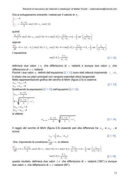
Ora si svilupperanno entrambi i metodi per il calcolo di θ p .
⎧τ
' '=
0
x y
⎪
⎨ σx+ σ y
⎪τ
' '=−
⋅sin 2⋅ + τ xy ⋅cos 2⋅
xy ⎩ 2
( θ ) ( θ )
quindi:
σx + σ y 2⋅τ 1 ⎛ xy τ ⎞
−1 xy
− ⋅sin( 2⋅ θ) + τxy ⋅cos( 2⋅ θ) = 0 ⇒ tan ( 2⋅ θp) = ⇒ θp=
⋅tan ⎜ ⎟
2 σ x −σ y 2 ⎜σ ⎟
⎝ x −σ
y ⎠
oppure:
d '
2 τ x 1 ⎛ xy τ ⎞
−1 xy
0 ( σx σ y) sin ( 2 θ) 2 τxy cos ( 2 θ) 0 tan ( 2 θp)
θ p tan
dθ
σx σ y 2 σx σ y
⋅
σ
= ⇒− − ⋅ ⋅ + ⋅ ⋅ ⋅ = ⇒ ⋅ = ⇒ = ⋅ ⎜
⎟
− − ⎟
⎝ ⎠
L’equazione:
2⋅τ
xy
tan ( 2⋅
θ p ) =
[2.1.12]
σ −σ
x y
definisce due valori 2 ⋅ θ p che differiscono di π radianti e dunque due valori θ p che
differiscono di π /2 radianti.
Poiché i due valori θ p definiti dall’equazione [2.1.12] sono stati ottenuti imponendo τ ' '=
0 ,
è chiaro che sui piani principali non vengono esercitati sforzi tangenziali.
Nella rappresentazione grafica del cerchio di Mohr (figura 2.5) si osserva:
σ = σ + R
max
min
med
σ = σ −R
med
Sostituendo le espressioni [2.1.10] nell’equazioni [2.1.13]:
⎧ σx + σ y
⎪σ
med =
⎪
2
⎪
2
⎪ ⎛σx + σ y ⎞ 2
⎨R = ⎜ ⎟ + τ xy
⎪ ⎝ 2 ⎠
⎪
⎪
σmax = σmed
+ R
⎪ ⎩σmin
= σmed
−R
si ottiene:
σx + σ y ⎛σx + σ y ⎞
σ max,min = ± ⎜ ⎟ + τ
2 ⎝ 2 ⎠
2
2
xy
xy
[2.1.13]
[2.1.14]
Il raggio del cerchio di Mohr (figura 2.5) essendo pari alla differenza tra σ max e σ min , si
scrive:
1
τmax = ⋅( σmax − σmin
)
2
[2.1.15]
dτ
' '
xy
Ora, imponendo la condizione
dθ
0 , si ottiene:
=
dτ
' '
xy
dθ
σx + σ y 2⋅τ 1 ⎛ xy τ ⎞
−1 xy
= 0 ⇒ ⋅cos( 2⋅ θ) + τxy ⋅sin ( 2⋅ θ) = 0 ⇒ tan ( 2⋅ θs) = ⇒ θs=
⋅tan ⎜ ⎟
2 σx −σ y 2 ⎜σx −σ
⎟
⎝ y ⎠
2⋅τ
xy
tan ( 2⋅
θs
) =
σ −σ
[2.1.16]
x y
questo risultato, definisce due valori 2⋅ θs
che differiscono di π radianti (180°) e dunque
due valori θ s che differiscono di π /2 radianti (90°).
13