Our automation system for a continuous tandem mill coupled with ...
Our automation system for a continuous tandem mill coupled with ...
Our automation system for a continuous tandem mill coupled with ...

You also want an ePaper? Increase the reach of your titles
YUMPU automatically turns print PDFs into web optimized ePapers that Google loves.
16<br />
Roberta Gatti & Sergio Murgia<br />
<strong>Our</strong> <strong>automation</strong> <strong>system</strong><br />
<strong>for</strong> a <strong>continuous</strong><br />
<strong>tandem</strong> <strong>mill</strong> <strong>coupled</strong><br />
<strong>with</strong> pickling line<br />
INTRODUCTION<br />
The cold rolling is one of the main sectors <strong>for</strong> rolling flat<br />
products. In the last 3 years Ansaldo Sistemi Industriali (ASI)<br />
acquired 20 cold rolling plants, of which 17 from a major<br />
Chinese customer, who demonstrated to be very satisfied of<br />
our <strong>automation</strong> <strong>system</strong>s developed in our Genoa factory<br />
(<strong>with</strong> the support of our office in Beijing). The paper presents<br />
the state of art of what is normally considered the most comprehensive<br />
and significant type of cold rolling plant: the <strong>continuous</strong><br />
<strong>tandem</strong> <strong>mill</strong> <strong>coupled</strong> <strong>with</strong> pickling line. In Italy we<br />
call it decatreno (fig. 1).<br />
THE PLANT AND ITS REQUIREMENTS<br />
The purpose of a cold rolling <strong>mill</strong> is to reduce the thickness<br />
of the entering coils of steel (coming from a hot strip <strong>mill</strong>) to<br />
a defined target <strong>with</strong> great accuracy, guaranteeing the best surface<br />
quality of the final strip and high plant productivity: note<br />
that a rolling <strong>mill</strong> usually works 24h/7d.<br />
There are more than one different type of <strong>mill</strong>s able to reach<br />
these targets, smaller or larger depending on productivity and<br />
final product characteristics. The largest one is composed by<br />
a set of rolling stands (usually 5) able to reduce the steel thickness<br />
by means of pressure (fig. 2, rolling <strong>for</strong>ce), created by hy-<br />
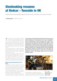
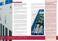
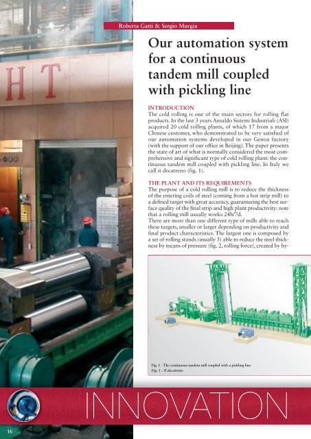
Fig. 1 - The <strong>continuous</strong> <strong>tandem</strong> <strong>mill</strong> <strong>coupled</strong> <strong>with</strong> a pickling line.<br />
Fig. 1 - Il decatreno<br />
INNOVATION
draulic capsules and exercised by 2 work rolls on the strip<br />
itself; and by means of the tensions between one stand and<br />
the others (interstand tensions); 4 or, as in the picture, 6 rolls<br />
in total are present in each stand <strong>for</strong> giving the suitable stiffness<br />
to the whole assembly.<br />
The plant inserted in fig. 2 is a coil-to-coil <strong>tandem</strong> <strong>mill</strong>:<br />
each coil is inserted into the <strong>mill</strong>, is rolled and is extracted<br />
when it has finished. Its productivity, in addition to stability<br />
of operations, can definitively increase if the coil-to-coil<br />
process is trans<strong>for</strong>med into a <strong>continuous</strong> process by welding<br />
the head of a coil to the tail of the previous one: in this<br />
way, the <strong>tandem</strong> can roll <strong>continuous</strong>ly, <strong>with</strong>out stopping<br />
and restarting when a coil finishes. Because welding machines<br />
require the strip to stop <strong>for</strong> a while, an accumulator<br />
(looper) is necessary in order to not stop rolling at the <strong>tandem</strong><br />
<strong>mill</strong> (see fig. 1, where vertical loopers are showed, but<br />
horizontal structures are often used).<br />
A flying shear located at <strong>tandem</strong> exit cuts the strip when a<br />
new coil has been <strong>for</strong>med on the coiler so that the process<br />
turns back to be dis<strong>continuous</strong>. Much time can pass after<br />
hot rolling and be<strong>for</strong>e cold process, rust is <strong>for</strong>med on the<br />
metal and it must be eliminated from the surface of the<br />
strip be<strong>for</strong>e it is rolled by having the strip passed inside<br />
tanks filled <strong>with</strong> a solution of water and hydrochloric acid;<br />
this can be done in pickling line be<strong>for</strong>e the coils reaches<br />
the <strong>tandem</strong> <strong>mill</strong>, or, more efficiently, the pickling line can<br />
be directly inserted between the welding machine and the<br />
1 st stand; additional loopers are required upstream of the<br />
stands to decouple the different phases giving maximum<br />
flexibility to such a plant, which can now reach 300 m<br />
length and accumulate 2000 m of strip in the loopers (see<br />
again fig. 1).<br />
Il nostro sistema<br />
di automazione<br />
per un decatreno<br />
INTRODUZIONE<br />
La laminazione a freddo è uno dei principali settori<br />
della laminazione dei prodotti piani ed ASI ha acquisito,<br />
negli ultimi 3 anni, 20 impianti di questo tipo,<br />
di cui ben 17 da un grosso cliente cinese, particolarmente<br />
soddisfatto dei nostri sistemi di automazione;<br />
questi vengono sviluppati dai colleghi della sede di<br />
Genova (col supporto della sede di Pechino) e l’articolo<br />
si pone lo scopo di illustrare lo stato dell’arte di<br />
quello che è normalmente ritenuto il più completo e<br />
significativo dei numerosi impianti dell’area a freddo,<br />
il <strong>tandem</strong> continuo con decapaggio; noi italiani lo abbreviamo<br />
con decatreno (fig. 1).<br />
L’IMPIANTO E I SUOI REQUISITI<br />
Lo scopo del laminatoio a freddo (chiamato anche<br />
<strong>tandem</strong> a freddo) è di ridurre ad un ben definito target<br />
e con grande accuratezza lo spessore dei rotoli di<br />
acciaio in ingresso (provenienti da un laminatoio a<br />
caldo), garantendo la migliore qualità superficiale del<br />
nastro finale ed una elevata produttività dell’impianto:<br />
si noti che un laminatoio normalmente lavora<br />
24 ore al giorno, 7 giorni su 7.<br />
Esistono vari tipi di laminatoi capaci di raggiungere<br />
questi target, più o meno grandi a seconda della produttività<br />
e delle caratteristiche del prodotto finale.<br />
Il più grande è composto da un certo numero di gabbie<br />
di laminazione (di solito sono 5) che riducono lo<br />
spessore dell’acciaio sia per mezzo della pressione<br />
(fig. 2, rolling <strong>for</strong>ce) generata da capsule idrauliche<br />
ed esercitata sul nastro da due cilindri di lavoro<br />
(work rolls) che per mezzo dei tiri tra una gabbia e<br />
l’altra (interstand tension); in ciascuna gabbia ci sono<br />
4 o, come in figura, 6 cilindri per conferire una adeguata<br />
rigidità all’intera struttura.<br />
L’impianto mostrato in fig. 2 è un laminatoio coil-tocoil:<br />
ogni rotolo viene introdotto nel laminatoio,<br />
viene laminato ed estratto una volta che è terminato.<br />
La produttività, oltre che la stabilità delle operazioni,<br />
può certamente aumentare se il processo discontinuo<br />
coil-to-coil viene tras<strong>for</strong>mato in continuo, e questo si<br />
fa saldando la testa di un rotolo alla coda del rotolo<br />
che lo precede: così facendo, il <strong>tandem</strong> può laminare<br />
continuativamente, senza doversi fermare e ripartire<br />
ogni volta che il rotolo finisce.<br />
Poiché le saldatrici richiedono che il nastro si fermi per<br />
un poco per la saldatura, è necessario un accumulatore<br />
(looper) per non far fermare la laminazione al <strong>tandem</strong><br />
quando il nastro è fermo alla saldatrice (in fig. 1 sono<br />
mostrati looper verticali, ma più spesso si utilizzano<br />
strutture orizzontali). Una cesoia volante (flying shear)<br />
all’uscita del <strong>tandem</strong> taglia il nastro quando un nuovo<br />
rotolo sull’aspo avvolgitore si è completato e il processo<br />
ritorna così ad essere discontinuo.<br />
17
18<br />
Rolling <strong>for</strong>ce<br />
Interstand tension<br />
Fig. 2 - Tandem <strong>mill</strong> applies <strong>for</strong>ces and tensions to reduce the strip thickness.<br />
Fig. 2 - Il laminatoio riduce lo spessore del nastro per mezzo di <strong>for</strong>ze e di tiri<br />
A few numbers taken from a typical plant can give an<br />
idea of the complexity of the cold rolling process and,<br />
as a consequence, of its <strong>automation</strong> <strong>system</strong> (tab. 1):<br />
this real-time control <strong>system</strong> must deal <strong>with</strong> a highlyinterconnected<br />
fast process and must guarantee accuracy,<br />
reliability and productivity by means of efficient<br />
generation of references <strong>for</strong> a large number of control<br />
loops able to run at cycle times of a few ms, connected<br />
to many actuators, sensors and supervision stations.<br />
Entry thickness 5.5 ÷ 2 mm<br />
Exit thickness 1.5 ÷ 0.14 mm<br />
Thickness measure accuracy ± 0.01 %<br />
Total thickness reduction up to 90 %<br />
Exit speed 20 m/s<br />
Main motor power (5 stands) 15 ÷ 30 MW<br />
Rolling <strong>for</strong>ces 10,000 kN<br />
Interstand tensions 100 ÷ 250 MPa<br />
Thickness per<strong>for</strong>mances ± 1 ÷ 3 % exit thickness in 98 %<br />
of the strip body<br />
Flatness per<strong>for</strong>mances (see details ± 8 ÷ 12 I.U. (fiber differential<br />
in the Flatness paragraph) elongation = ± 80 ÷ 120 μm<br />
per 1 rolled meter)<br />
Production 1.2 <strong>mill</strong>ions tons per year<br />
Tab. 1 - Some typical data summarize the high-demanding capabilities requested<br />
from a modern cold rolling <strong>mill</strong><br />
Tab. 1 - Alcuni valori tipici riassumono le stringenti richieste di prestazioni per<br />
un moderno laminatoio a freddo<br />
Roberta Gatti & Sergio Murgia<br />
Work rolls<br />
Rolling stand<br />
THE AUTOMATION SYSTEM<br />
Fig. 3 illustrates in a very simplified way the theoretical<br />
scheme of our <strong>automation</strong> <strong>system</strong>s, while fig. 4 presents<br />
the <strong>automation</strong> layout <strong>for</strong> the <strong>continuous</strong> <strong>mill</strong>:<br />
• Level 1: includes many regulators which control position<br />
or pressure of the hydraulic capsules, tension<br />
and thickness of the strip, speeds of the motors, and<br />
so on: inner and outer loops, concurrent loops, decoupling<br />
actions and on-line gain calibrations are<br />
often necessary; the level 1 also manages logic, sequences,<br />
hydraulics, communication <strong>with</strong> the field<br />
(sensors, actuators, electrical drives, operator desks,<br />
etc.). Data acquisition is used to investigate details<br />
in regulators.<br />
• Level 2: the references to be sent to the regulators<br />
change depending on the different products to be<br />
rolled (production programs comes from the production<br />
management department – level 3) and/or<br />
due to the intrinsic tempo-variance of the plant (e.g.,<br />
work rolls heat up and wear) so that they are recalculated<br />
by dedicated mathematical models <strong>for</strong> each<br />
new piece (consider many tens of pieces per day);<br />
measures are collected <strong>for</strong> autoadapting the models<br />
piece-by-piece and <strong>for</strong> certifying the quality of each<br />
coil produced.<br />
INNOVATION
Spesso passa parecchio tempo tra la laminazione a caldo e<br />
quella a freddo, per cui sul metallo si <strong>for</strong>ma della ruggine<br />
che deve essere eliminata facendo passare il nastro dentro<br />
alcune vasche con una soluzione di acqua e acido cloridrico;<br />
questo processo di decapaggio (pickling line) può essere<br />
fatto in un altro impianto prima di laminare il nastro al <strong>tandem</strong><br />
o, più efficientemente, il decapaggio può essere inserito<br />
direttamente tra la saldatrice e la prima gabbia; servono<br />
dunque altri looper prima delle gabbie per disaccoppiare le<br />
diverse fasi e conferire così il massimo di flessibilità all’impianto,<br />
che ora può raggiungere i 300 m in lunghezza ed accumulare<br />
2000 m di nastro nei looper (v. ancora fig. 1).<br />
Alcune cifre di un tipico impianto possono dare l’idea della<br />
complessità del processo di laminazione a freddo e, di conseguenza,<br />
del suo sistema di automazione (tab. 1): questi<br />
controlli in real-time devono gestire un processo veloce ed<br />
altamente interconnesso e devono garantire accuratezza,<br />
affidabilità e produttività per mezzo di una efficiente generazione<br />
dei riferimenti per un gran numero di anelli di<br />
regolazione che girano a tempi di ciclo dell’ordine di pochi<br />
ms, connessi ad altrettanto numerosi attuatori, sensori e<br />
stazioni di supervisione.<br />
IL SISTEMA DI AUTOMAZIONE<br />
La fig. 3 illustra in maniera molto semplificata lo schema<br />
teorico dei nostri sistemi di automazione , mentre la fig. 4<br />
presenta la configurazione di automazione per un decatreno:<br />
• Livello 1: comprende molti regolatori che controllano posizioni<br />
e pressioni delle capsule idrauliche, tiri e spessori<br />
del nastro, velocità dei motori e così via; spesso sono necessari<br />
anelli interni ed esterni, anelli concorrenti, azioni<br />
di disaccoppiamento e calibrazioni on-line; il livello 1 gestisce<br />
anche le logiche, le sequenze, le idrauliche, le comunicazioni<br />
col campo (sensori, attuatori, azionamenti<br />
elettrici, banchi operatore, ecc.). Un completo sistema di<br />
acquisizione dati consente di investigare accuratamente i<br />
dettagli di comportamento dei regolatori .<br />
• Livello 2: i riferimenti necessari ai regolatori possono<br />
cambiare a seconda dei diversi prodotti da laminare (i<br />
programmi di produzione arrivano dal dipartimento che<br />
gestisce la produzione – livello 3) e/o a causa della intrinseca<br />
tempo-varianza dell’impianto (p. es., i cilindri di lavoro<br />
si scaldano e si usurano); i riferimenti vengono<br />
dunque ricalcolati pezzo per pezzo (e si laminano molte<br />
decine di pezzi al giorno) da modelli matematici appositamente<br />
sviluppati; durante la laminazione vengono raccolte<br />
moltissime misure sia per auto-adattare i modelli<br />
matematici pezzo dopo pezzo, sia per certificare la qualità<br />
di ciascun nastro prodotto.<br />
Le caratteristiche peculiari che contraddistinguono il <strong>tandem</strong><br />
continuo possono essere ora brevemente descritte per aggiun-<br />
gere in<strong>for</strong>mazioni pratiche al precedente schema teorico.<br />
Calcolo del setup e funzioni di livello 2 di base<br />
La scheda di laminazione che contiene i riferimenti che il<br />
livello 1 deve attuare viene calcolata da accurati modelli<br />
matematici quando il rotolo viene saldato, quando si trova<br />
al decapaggio e prima di entrare nel <strong>tandem</strong>; i calcoli necessari<br />
al meccanismo di auto-adattamento dei modelli matematici<br />
sono effettuati quando il rotolo finito viene<br />
tagliato e lascia il <strong>tandem</strong>, usando le misure acquisite durante<br />
il suo processamento. Inoltre, i server di processo raccolgono,<br />
gestiscono e immagazzinano tutti i dati relativi a<br />
ciascun rotolo laminato (dati primari, scheda di laminazione,<br />
calcoli di adattamento, riferimenti applicati, misure<br />
di qualità) e alla produzione effettuata. Gestiscono anche<br />
la connessione col sistema di automazione di livello 3.<br />
Cambio di Set al Volo<br />
Il mondo dei modelli matematici e dell’attuazione dei riferimenti<br />
per i laminatoi è parecchio ampio e variegato, ma<br />
ciò che sicuramente fa la differenza in un laminatoio continuo<br />
è il cambio di set al volo, che coinvolge sia capacità<br />
modellistiche che regolazioni e logiche real-time. La scheda<br />
di laminazione, calcolata per ciascun nastro, assicura riferimenti<br />
ottimali per quel nastro; ma quando la saldatura<br />
tra due diversi nastri passa attraverso le gabbie, il punto<br />
operativo dell’impianto si deve spostare dallo stato del nastro<br />
corrente a quello del successivo e questo cambio deve<br />
essere continuamente gestito dal sistema di automazione.<br />
Diversi set intermedi (v. fig. 5), calcolati dai modelli matematici<br />
e applicati al momento giusto dai regolatori mentre<br />
la saldatura si muove attraverso il <strong>tandem</strong>, permettono di<br />
mantenere la stabilità di laminazione (limitando il rischio<br />
di rottura nastro) per minimizzare la lunghezza di nastro<br />
fuori tolleranza, limitando l’area di transizione e massimizzando<br />
la produzione.<br />
Controllo Automatico di Spessore & Controllo di Tiro<br />
(AGC & ATC)<br />
Lo spessore del prodotto finito che sta in tolleranza è ciò<br />
che appare immediatamente al cliente finale e ha fondamentale<br />
importanza sia per quel che riguarda la qualità del nastro<br />
che per la bontà complessiva dell’impianto (v. fig. 6). I<br />
modelli matematici calcolano riduzioni nominali e tiri intergabbia<br />
al fine di ottenere le condizioni operative desiderate<br />
in assenza di disturbi. I controlli tecnologici sono<br />
progettati per minimizzare le variazioni che sorgono durante<br />
la laminazione: per esempio, variazioni di spessore e<br />
di durezza del materiale d’ingresso, fenomeni termici sui<br />
cilindri di lavoro, usura ed eccentricità dei cilindri e variazioni<br />
di attrito, se non vengono adeguatamente controllati<br />
dal sistema di automazione, provocano deviazioni di spessore<br />
dal target garantito per il prodotto finale (fig. 7).<br />
Nella fig. 8 è mostrato il sistema di controllo: sono eviden-<br />
19
20<br />
REPORTS<br />
MATHEMATICAL<br />
MODELS<br />
Level 2<br />
Production Programs<br />
Production Reports<br />
The peculiar features that distinguish the <strong>continuous</strong><br />
<strong>tandem</strong> <strong>mill</strong> can be now briefly described <strong>for</strong> adding<br />
more practical in<strong>for</strong>mation to the previous theoretical<br />
scheme.<br />
+<br />
-<br />
Roberta Gatti & Sergio Murgia<br />
Level 1<br />
Level 3<br />
R<br />
R<br />
REGULATOR<br />
MODEL<br />
ADAPTION Adaption Measures<br />
Fig. 3 - Functional structure of the <strong>automation</strong> <strong>system</strong> Fig. 3 - Struttura funzionale del sistema di automazione<br />
OPERATOR STATIONS<br />
& LOCAL CONTROL DESKS<br />
LEVEL 2<br />
& COMPUTER ROOM<br />
LEVEL 1<br />
LEVEL 0/PLANT<br />
Entry pulpit<br />
LEVEL 3 NETWORK<br />
(to level 3 <strong>system</strong>)<br />
Entry and<br />
pickling areas<br />
Process<br />
Servers<br />
Setup Calculation and<br />
Level 2 Basic Functions<br />
The rolling schedule to<br />
be actuated by level 1 is<br />
calculated by accurate<br />
mathematical models<br />
when the coil is welded,<br />
when it is at the pickling<br />
line and be<strong>for</strong>e entering<br />
the <strong>tandem</strong> <strong>mill</strong>; calcula-<br />
PLANT<br />
tions dedicated to autoadapt<br />
the mathematical<br />
models using actual plant<br />
measures are carried out<br />
when the coil is cut and<br />
exits the plant. In addition,<br />
the process servers<br />
are dedicated to collect,<br />
manage and store all of<br />
the in<strong>for</strong>mation related<br />
to each coil (primary<br />
data, rolling schedules, adaption calculations, applied<br />
sets, quality measures) and to production and operations.<br />
They also manage the connection to the level 3<br />
<strong>system</strong>.<br />
HMI NETWORK<br />
DATA ACQUISITION NETWORK<br />
Maintenance<br />
stations<br />
Side trimmer<br />
pulpit Tandem pulpit<br />
HMI Servers<br />
MAIN NETWORK<br />
Engineering<br />
stations<br />
Drives Drives<br />
Data<br />
acquisition<br />
client<br />
Fig. 4 - ASI <strong>automation</strong> <strong>system</strong> <strong>for</strong> a cold <strong>tandem</strong> <strong>mill</strong> <strong>coupled</strong> <strong>with</strong> pickling line Fig. 4 - Il sistema di automazione ASI per un decatreno<br />
Fast I/O<br />
Tandem<br />
area<br />
COMMUNICATION NETWORK FIELD NETWORK<br />
Slow I/O<br />
INNOVATION
ziati i relativi sensori e le funzioni principali.<br />
L’ATC (Controllo Automatico di Tiro) ha lo scopo di mantenere<br />
il tiro ben vicino al riferimento calcolato dai modelli<br />
matematici e di prevenire rotture del nastro. Un rullo tensiometrico,<br />
posizionato in ciascuna intergabbia, <strong>for</strong>nisce la<br />
misura di tiro.<br />
Sia la velocità delle gabbie che la luce tra i cilindri agiscono<br />
sui tiri intergabbia: sono così usati due diversi regolatori:<br />
• Controllo di tiro tramite carico: agisce su posizione o<br />
<strong>for</strong>za dei cilindri della gabbia a valle (HGC – Controllo<br />
Idraulico di Posizione - in fig. 8).<br />
• Controllo di tiro tramite velocità: agisce sulla velocità<br />
delle gabbie a valle o a monte (non mostrato in fig. 8);<br />
Il primo regolatore è usato a bassa velocità, quando sono<br />
presenti diverse condizioni di laminazione: il coefficiente<br />
di attrito tra cilindri di lavoro e nastro è così grande che il<br />
controllo di tiro tramite carico richiederebbe correzioni di<br />
<strong>for</strong>za eccessive e danneggerebbe la planarità del nastro.<br />
L’ATC tramite carico lavora a velocità più alta. La commutazione<br />
da una modalità all’altra avviene in maniera automatica.<br />
Una differenziazione va fatta quando il <strong>tandem</strong> lamina con<br />
basse riduzioni sull’ultima gabbia: in questa situazione è preferibile<br />
controllare il tiro dell’ultima intergabbia agendo solo<br />
sulla velocità della gabbia 4 (indipendentemente dalla velocità<br />
di laminazione) così che il controllo di posizione sull’ultima<br />
gabbia sia disponibile per il controllo di planarità.<br />
L’AGC (Controllo Automatico di Spessore) riceve la misura<br />
di deviazione di spessore dai misuratori a raggi X. A<br />
differenza del tiro, lo spessore non viene misurato all’uscita<br />
di ogni gabbia a causa dei costi elevati e dei rischi di danneggiamento<br />
in casi di strappo del nastro. La configurazione<br />
tipica prevede tre misuratori (v. fig. 8 per il loro<br />
posizionamento).<br />
L’AGC comprende due sottosistemi principali:<br />
• AGC di ingresso: ha lo scopo di mantenere il corretto<br />
spessore del nastro all’uscita dalla prima gabbia, usando<br />
le misure che arrivano dai primi due misuratori.<br />
• AGC di uscita: controlla lo spessore del nastro all’uscita<br />
dal <strong>tandem</strong> usando la misura dell’ultimo sensore e<br />
agendo sulla velocità delle ultime due gabbie.<br />
Infine, il monitor AGC ha lo scopo di riportare nei limiti<br />
la correzione dell’AGC di uscita nel caso in cui entri in regione<br />
di pre-saturazione; il monitor, in pratica, ricalibra il<br />
target di spessore dell’AGC di ingresso così da risistemare<br />
il flusso di materiale che entra nel <strong>tandem</strong> in accordo con<br />
i requisiti dell’AGC di uscita.<br />
È fondamentale, per i <strong>tandem</strong> a freddo, che l’errore di spessore<br />
all’uscita della prima gabbia sia mantenuto costante,<br />
anche se non nullo, poiché l’AGC di uscita è perfettamente<br />
in grado di correggere deviazioni di spessore molto lente,<br />
ma è meno efficace per correggere errori occasionali dato<br />
che la sua dinamica è limitata dai ritardi di trasporto tra<br />
l’ultima gabbia (su cui il controllo opera) e il misuratore di<br />
spessore: l’errore di spessore, infatti, prima di essere rilevato<br />
deve arrivare dalla gabbia al misuratore, per cui<br />
l’azione di controllo deve necessariamente essere lenta per<br />
evitare l’insorgere di instabilità.<br />
La presenza di sofisticati misuratori di velocità (laser) a<br />
monte e a valle della prima gabbia consente all’AGC massflow<br />
di applicare azioni di controllo veloci sull’HGC della<br />
prima gabbia. L’AGC massflow si basa sul principio di conservazione<br />
della portata di metallo (massflow), il che significa<br />
che la quantità di materiale che entra nella gabbia è<br />
uguale a quella che esce. E poiché nella laminazione a freddo<br />
la larghezza del nastro non varia, è possibile scrivere:<br />
h IN · v IN = h OUT · v OUT<br />
dove hIN = spessore d’ingresso;<br />
hOUT = spessore d’uscita;<br />
vIN = velocità lineare del nastro in ingresso;<br />
hOUT = velocità lineare del nastro in uscita.<br />
L’AGC massflow corregge l’errore<br />
εmassflow = vIN _ h* OUT<br />
v OUT<br />
h IN<br />
dove<br />
h* OUT = spessore nominale in uscita dalla prima gabbia.<br />
Chiaramente, azzerare ε massflow significa far sì che lo spessore<br />
che esce dalla prima gabbia sia uguale al riferimento<br />
calcolato dai modelli matematici.<br />
Stiamo gestendo anche guasti a sensori delicate come i misuratori<br />
laser di velocità, usando al loro posto gli encoder<br />
che sono sempre presenti sulla briglia d’ingresso e sulla<br />
gabbia. L’AGC massflow può così ottenere ottime prestazioni<br />
anche in assenza dei misuratori laser di velocità: per<br />
esempio, i grafici di fig. 6 (tratti da un <strong>tandem</strong> senza misuratori<br />
laser di velocità) mostrano come lo spessore in<br />
uscita dalla prima gabbia sia mantenuto comunque costante<br />
malgrado i cambi nello spessore d’ingresso e nella<br />
velocità di laminazione.<br />
L’AGC massflow può agire accoppiato ad una funzione di<br />
monitor (monitor di massflow) che ha lo scopo di compensare<br />
errori di valutazione del massflow (errori di misura,<br />
slittamenti, …) basandosi sulla misura di deviazione di spessore<br />
proveniente dal misuratore a valle della prima gabbia.<br />
Controllo Automatico di Planarità (AFC)<br />
La planarità del nastro, con lo spessore, è la più importante<br />
caratteristica del prodotto a cui il mercato dell’acciaio è<br />
estremamente sensibile. Il requisito di base è che il nastro laminato<br />
a freddo sia piano e completamente privo di curvature;<br />
nel prodotto finale ci saranno, infatti, difetti di<br />
planarità se gli stress residui dopo la laminazione eccederanno<br />
certi valori critici. In questi casi, il nastro mostrerà difetti<br />
di planarità come onde laterali o sfondamenti centrali.<br />
21
22<br />
Flying Setup Change<br />
The world of the mathematical models and references<br />
actuation <strong>for</strong> rolling <strong>mill</strong>s is quite wide and variegated,<br />
but what surely makes the difference in a <strong>continuous</strong><br />
<strong>tandem</strong> <strong>mill</strong> is the flying setup change, that involves<br />
both modelling capabilities and real-time regulation<br />
and logic. The rolling schedule calculated <strong>for</strong> each coil<br />
to be rolled ensures the optimal references <strong>for</strong> that<br />
coil; but when the weld seam between two different<br />
coils passes through the stands, the <strong>mill</strong> operating<br />
point must move from the current state to the future<br />
state of the next product and the change has to be <strong>continuous</strong>ly<br />
managed by the <strong>automation</strong> <strong>system</strong>. Different<br />
intermediate sets (see fig. 5), calculated by<br />
mathematical models and applied in the correct moments<br />
by regulators while weld seam moves along the<br />
<strong>mill</strong>, allow to maintain rolling stability (limiting the<br />
risk of strip breakage), to minimize the length of offspecification<br />
rolled strip by limiting the transition area<br />
and to maximize the production.<br />
Automatic Gauge Control & Tension Control (AGC<br />
& ATC)<br />
The in-tolerance thickness of the final product is what<br />
immediately appears to the final customers and has a<br />
fundamental importance both on the strip quality and<br />
on the entire plant bounty (fig. 6). The mathematical<br />
models calculate the nominal stand reductions and interstand<br />
tensions in order to get the desired operating<br />
conditions in the absence of disturbances.<br />
The technological controls are designed to minimise<br />
the variations which occur during rolling: <strong>for</strong> example,<br />
thickness and hardness variations in the entry strip,<br />
thermal phenomena affecting the work rolls, roll wear,<br />
roll eccentricity and friction variations cause deviations<br />
from the guaranteed target thickness in the final<br />
product if not adequately controlled by the <strong>automation</strong><br />
<strong>system</strong> (fig. 7).<br />
The control <strong>system</strong> is shown in figure 8: the relevant<br />
sensors and the main functions are pointed out.<br />
ATC (Automatic Tension control) is aimed to maintain<br />
tension close to the reference calculated by mathematical<br />
models and to prevent strip breaks. A tensionmeter<br />
roll located in each interstand supplies the<br />
tension feedback.<br />
Both stand speeds and stand rollgap positions affect<br />
the interstand tensions: two different controllers are<br />
then used:<br />
• Tension control by load: operates by adjusting the<br />
rollgap position/<strong>for</strong>ce of the downstream stand<br />
(HGC - Hydraulic Gap Control - in fig. 8).<br />
Roberta Gatti & Sergio Murgia<br />
• Tension control by speed: operates by adjusting the<br />
speed of the upstream or downstream stand (not<br />
shown in fig. 8);<br />
The first regulator is used at low speed, when different<br />
rolling conditions are present: the friction coefficient<br />
between work rolls and strip is so high that the tension<br />
control by load would require excessive corrections of<br />
<strong>for</strong>ce, thus affecting strip flatness. ATC by load operates<br />
at higher speed. The switch from one mode to the<br />
other one is automatic.<br />
A distinction must be done <strong>for</strong> the last interstand<br />
when the <strong>mill</strong> rolls steel sheet <strong>with</strong> a small reduction<br />
at the last stand: in this situation, it is preferable to<br />
control tension by acting on stand 4 speed only (independently<br />
on the rolling speed), so that the rollgap on<br />
the last stand is available <strong>for</strong> shape control.<br />
AGC (Automatic Gauge Control) gets thickness deviation<br />
feedback from x-ray gauges. Unlike tension,<br />
thickness is not measured at the exit of all stands, due<br />
to the cost and the risk of damage during strip breakages.<br />
The typical plant configuration <strong>for</strong>esees three<br />
gauges (see fig. 8 <strong>for</strong> their location).<br />
AGC includes two main sub<strong>system</strong>s:<br />
• Entry AGC: is aimed to maintain a consistent strip<br />
thickness at stand 1 exit, by using the feedbacks coming<br />
from the first two x-rays.<br />
• Exit AGC: it controls the strip thickness at <strong>mill</strong> exit,<br />
by using the feedback coming from the last x-ray. and<br />
acting on the last stands speed.<br />
Moreover, AGC Monitor aims to bring the Exit AGC<br />
correction in range when it enters into a pre-saturation<br />
region; it recalibrates the Entry AGC thickness target,<br />
thus adjusting the material flow entering the <strong>mill</strong> according<br />
to the requirements of Exit AGC.<br />
For <strong>tandem</strong> <strong>mill</strong>s it is fundamental that the thickness<br />
error at the exit of stand 1 is kept constant, even if not<br />
null, as the Exit AGC is perfectly able to compensate<br />
very slow deviations, but it is less effective <strong>for</strong> occasional<br />
errors, being its dynamics limited by the transport<br />
delay between the last stand (on which the<br />
control operates) and the exit thickness gauge: the<br />
thickness error has to travel from the stand to the<br />
gauge be<strong>for</strong>e being detected; because of this, the control<br />
action must be slow to avoid instability.<br />
The presence of accurate strip speed sensors (such as<br />
laser speedometers) at stand 1 entry and exit allows<br />
Massflow AGC to apply fast control action on stand<br />
1 HGC. Massflow AGC is based on massflow constancy<br />
principle, i.e. the material entering the stand is<br />
equal to the one going out of the stand.<br />
INNOVATION
Fig. 5 - A weld is passing through the <strong>mill</strong>: the change of references is calculated<br />
and applied stand by stand.<br />
Fig. 5 - Una saldatura sta passando attraverso le gabbie: il cambio di riferimenti<br />
viene calcolato ed applicato gabbia per gabbia.<br />
Fig. 6 - A minimum thickness of 140μm has been reached during a test aimed at<br />
demonstrating the feasibility of so a thin thickness in a <strong>tandem</strong> <strong>mill</strong> (Continuous<br />
Tandem Mill - PRC).<br />
Fig. 6 - Lo spessore minimo di 140μm è stato ottenuto in un test volto a dimostrare<br />
la capacità dell’impianto di realizzare uno spessore così sottile<br />
in un <strong>tandem</strong> a freddo (Tandem Continuo - Cina).<br />
Fig. 7 - A coil <strong>with</strong> non-uni<strong>for</strong>m thickness (e.g., due to skid marks at hot rolling)<br />
enters the 1st stand: AGC works very effectively so to bring the exit thickness<br />
<strong>with</strong>in the tolerances (Tandem Mill - Italy)<br />
Fig. 7 - Un nastro con spessore non uni<strong>for</strong>me (p. es., a causa di skid-marks durante<br />
la laminazione a caldo) entra nella prima gabbia: l’AGC lavora<br />
molto efficientemente e mantiene lo spessore entro le tolleranze (Tandem<br />
- Italy)<br />
23
24<br />
Mass Flow<br />
HGC 1<br />
Mass Flow Monitor<br />
Roberta Gatti & Sergio Murgia<br />
HGC 2 HGC 3 HGC 4 HGC 5<br />
MASS FLOW AGC AGC MONITOR<br />
laser speedometer<br />
X-ray thickness gauge<br />
Monitor<br />
Speed 4 Speed 5<br />
tensiometer<br />
Feedback<br />
ATC<br />
by load<br />
EXIT AGC<br />
Fig. 8 - Thickness and Tension control at a glance Fig. 8 - Un colpo d’occhio sui controlli di spessore e di tiro<br />
Top view of the strip,<br />
fiber by fiber<br />
A fiber, side view<br />
S<br />
L<br />
Fig. 9 - Definition of strip flatness Fig. 9 - Definizione di planarità del nastro<br />
INNOVATION<br />
Le<br />
Le<br />
Lm
Fig. 10 - 3D representation of strip flatness error: note that every sample is in<br />
tolerance (±12 I.U.) (Continuous Tandem Mill - Italy)<br />
Fig. 10 - Rappresentazione tridimensionale dell’errore di planarità del nastro:<br />
si noti che tutti i campioni sono in tolleranza (±12 I.U.) (Tandem Continuo<br />
- Italia)<br />
As in cold rolling strip width remains constant, we can<br />
write:<br />
hIN · vIN = hOUT · vOUT where hIN: entry thickness,<br />
hOUT: exit thickness,<br />
vIN: strip entry linear speed,<br />
vOUT: strip exit linear speed.<br />
Then Massflow AGC considers as error the following:<br />
εmassflow = vIN _ h* OUT<br />
vOUT hIN where h* OUT: stand 1 exit nominal thickness.<br />
Clearly, nullifying εmassflow means obtaining strip exiting<br />
the 1st stand at the thickness calculated by the<br />
mathematical models.<br />
Failures in sensitive sensors such as laser speedometers<br />
are being handled through encoders that are present<br />
both on entry bridle and stand 1. Massflow AGC can<br />
reach very good per<strong>for</strong>mances also in absence of the<br />
laser speedometers: <strong>for</strong><br />
example, figure 6 (taken<br />
from a <strong>tandem</strong> <strong>mill</strong> <strong>with</strong>out<br />
lasers) shows that<br />
stand 1 exit thickness is<br />
maintained constant by<br />
the control in spite of the<br />
entry thickness changes<br />
and of the rolling speed<br />
changes.<br />
AGC Massflow can operate<br />
<strong>coupled</strong> <strong>with</strong> a<br />
monitor function (Massflow<br />
Monitor) aiming to<br />
compensate <strong>for</strong> the massflow<br />
estimation errors<br />
(measure errors, slipping…),<br />
basing on the<br />
thickness deviation feedback<br />
coming from the<br />
gauge at stand 1 exit.<br />
Automatic Flatness<br />
Control (AFC)<br />
The strip flatness is the<br />
most important product<br />
characteristic, along <strong>with</strong><br />
thickness, to which the<br />
steel market is extremely sensitive.<br />
A basic requirement is that the cold rolled strip must<br />
be flat and completely free of camber; flatness defects<br />
in the final product will occur if the residual stresses<br />
remaining after rolling exceed critical values.<br />
tension<br />
from the last<br />
stand<br />
<strong>for</strong>ces<br />
tension<br />
to Rewind Reel<br />
rolling direction<br />
Fig. 11 - Working scheme of the shapemeter: the rotors measure the vertical <strong>for</strong>ces<br />
Fig. 11 - Schema operativo dello shapemeter: i rotori misurano le <strong>for</strong>ze verticali<br />
25
26<br />
In this case, the strip will show flatness defects as wavy<br />
edges or centre buckles.<br />
Fig. 9 illustrates the flatness definition, while fig. 10<br />
shows a snapshot of the 3d representation of flatness<br />
measured during rolling.<br />
Consider that the guaranteed tolerances range around<br />
10 I.U. (International Units) and this means to detect<br />
and control a delta length between the wavy and the<br />
tight fibers of 1 mm only in a wave 10 meters long!<br />
Strip flatness is measured <strong>with</strong> a shapemeter: a segmented<br />
roll located at the 5th stand exit which measures,<br />
rotor by rotor, the vertical <strong>for</strong>ces to which the<br />
strip is subjected during rolling, across the width of<br />
the strip (see fig. 11); it is then mathematically possible<br />
to obtain the longitudinal tensions from the <strong>for</strong>ces<br />
and, from them, the flatness index of the strip.<br />
Roberta Gatti & Sergio Murgia<br />
Roll Selective Cooling Shapemeter<br />
Roll Bending<br />
Roll Shifting<br />
Tilting (differential gap)<br />
Asymmetric<br />
Symmetric<br />
Local<br />
ASI’s flatness control processes rough measurements<br />
coming from the shapemeter in order to extract the<br />
three components of the error that the available actuators<br />
can most efficiently correct (see fig. 12); bending<br />
and intermediate shifting quickly and accurately compensates<br />
<strong>for</strong> symmetrical defects, while tilting acts on<br />
the asymmetrical defects in the strip.<br />
Localized defects, usually a result of thermal phenomena,<br />
can be efficiently corrected by selective cooling<br />
sprays: they have a slow dynamic, but can act on a<br />
precise area of the strip.<br />
A Feed<strong>for</strong>ward Force Compensation function (FFC)<br />
calculates a further contribution of bending, taking<br />
into account that the <strong>for</strong>ce can change during rolling,<br />
e.g. due to corrections from AGC, or from ATC.<br />
Shape Signal<br />
Components<br />
Fig. 12 - The 3 components of shape error are corrected separately Fig. 12 - Le 3 componenti dell’errore di planarità sono corrette separatamente<br />
INNOVATION
La fig. 9 illustra la definizione di planarità, mentre la fig.<br />
10 mostra una rappresentazione tridimensionale della planarità<br />
misurata durante la laminazione. Si consideri che<br />
l’intervallo di tolleranza garantito è intorno alle 10 I.U., il<br />
che significa rilevare e controllare una differenza di lunghezza<br />
tra la fibra ondeggiante e quella tesa di 1 solo mm<br />
su un’onda lunga 10 m!<br />
La planarità del nastro è misurata con uno shapemeter: si<br />
tratta di un rullo segmentato posizionato all’uscita della<br />
quinta gabbia in grado di misurare, rotore per rotore, le<br />
<strong>for</strong>ze verticali a cui il nastro è soggetto durante la laminazione,<br />
sulla larghezza del nastro stesso (v. fig. 11); dopodiché,<br />
dalle <strong>for</strong>ze è possibile calcolare matematicamente i<br />
tiri longitudinali e, da essi, l’indice di planarità del nastro.<br />
Il controllo di planarità di ASI processa le misure grezze<br />
provenienti dallo shapemeter ed estrae le tre componenti<br />
dell’errore che possono essere efficacemente correcti dagli<br />
attuatori disponibili (v. fig. 12); il bending e lo shifting intermedio<br />
sono in grado di correggere velocemente ed accuratamente<br />
i difetti simmetrici, mentre il tilting (posizione<br />
differenziale dei cilindri) agisce sui difetti asimmetrici del<br />
nastro. I difetti locali, che di solito sono il risultato di fenomeni<br />
termici, possono essere efficacemente corretti mediante<br />
il raffreddamento selettivo dei cilindri di lavoro:<br />
hanno una dinamica lenta, ma possono agire su ben precise<br />
zone del nastro. Infine, la funzione di compensazione<br />
di <strong>for</strong>za in anello aperto calcola un ulteriore contributo di<br />
bending in base alle variazioni di <strong>for</strong>za che possono avvenire<br />
durante la laminazione, p. es., dovute a correzioni dell’AGC<br />
o dell’ATC.<br />
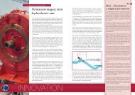
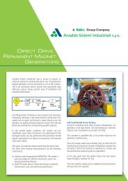
Fig. 13 - 5-Stand Tandem Mill (PRC) Fig. 13 - Tandem a 5 gabbie (China)<br />
27