Social Indicators of Equality for Minorities and Women - University of ...

Thurgood Marshall Law LibraryThe University of Maryland School of LawSocial indicatorsof Equality forMinorities and WomenReport of the United Stat

U.S. COMMISSION ON CIVIL RIGHTSThe U.S. Commission on Civil Rights is a temporary, independent, bipartisanagency established by Congress in 1957 and directed to:• Investigate complaints alleging that citizens are being deprived of their right tovote by reason of their race, color, religion, sex, or national origin, or by reason offraudulent practices;• Study and collect information concerning legal developments constituting adenial of equal protection of the laws under the Constitution because of race,color, religion, sex, or national origin, or in the administration of justice;• Appraise Federal laws and policies with respect to the denial of equalprotection of the laws because of race, color, religion, sex, or national origin, or inthe administration of justice;• Serve as a national clearinghouse for information in respect to denials of equalprotection of the laws because of race, color, religion, sex, or national origin;• Submit reports, findings, and recommendations to the President and theCongress.MEMBERS OF THE COMMISSIONArthur S. Flemming, ChairmanStephen Horn, Vice ChairmanFrankie M. FreemanManuel Ruiz, Jr.Murray SaltzmanLouis Nunez, Acting Staff Director

Letter of TransmittalU.S. COMMISSION ON CIVIL RIGHTSWashington, D.C.August 1978PRESIDENTPRESIDENT OF THE SENATESPEAKER OF THE HOUSE OF REPRESENTATIVES>SWie U.S. Commission on Civil Rights presents to you this report pursuant toPJMic Law 85-315, as amended.^ie information provided here stems from an awareness of the importance ofeHRiating efforts to improve the condition of our society in areas such as educationa^housing and an awareness that all too often the status of women and minoritymeji is obscured by statistics reflecting the society as a whole. The "social indicatorsoi^uality" presented in this report directly compare the level of well-being of thendfcprity and female population to that of the majority male population and, thus,as^ss the Nation's progress toward achieving equality.WFUT findings and recommendations regarding levels of equality are based onnAsures in the areas of education, occupation, employment, income, poverty, andhousing, developed from data from the State Public Use Samples Tapes of the 1960aWl970 censuses and from the 1976 Survey of Income and Education Public UseTapes. Our findings show that for every indicator reported here, women andmmp [ority men have a long way to go to reach equality with majority men, and, inmB[y instances, are relatively further from equality in 1976 than they were in 1960.recommendations are directed toward utilizing the detailed measurementspi^ented in the report and improving the Federal statistical system and socialinRator program. The President, as reported in his May 1L 1978, memorandum onof the Federal statistical system, already has taken a first step toward theseby directing his Reorganization Task Force to address the problems ofving the coordination and policy relevance of Federal statistical activities. Ourmendations seek to ensure that the Federal Government routinely calculatesanalyzes measures of equality in order to assess adequately the impact of socialeconomic reform programs and to ensure adequate and accurate representationo^^inorities in surveys seeking information on the state of the Nation. We alsommend that Federal officials in a variety of agencies consider our analyses asals of continuing severe social and economic inequality and review theirrams intended to remedy such conditions.e urge your attention to the information presented here and the use of youroffices in achieving the needed corrective action to facilitate our progressd achieving equality for all in the Nation.ectfully,S. Flemming, Chairmanlen Horn, Vice Chairman•• M. FreemanRuiz, Jr.ray SaltzmanNunez, Acting Staff Directorin

ACKNOWLEDGMENTSCommission is indebted to staff members Havens Tipps and Linda Zimbler,p prepared this report under the direction of Deborah P. Snow. The Commissionappreciates the contributions of Jose Hernandez, who supervised an early stageproject; the critical review provided by Professors Leo Estrada and Reynolds^ of a draft of the report; and the assistance of an advisory workshop,cWsisting of Professor Leo Estrada, Susan Gustavus Philliber, Bart Landry, SetsukoN^tsunaga Nishi, Clara Rodriguez, and Jay Stauss, in the initial formulation of thereject.TJ^ following staff members provided support in preparing the report: GloriaFarcer, Antoinette Foster, Patsy Washington, Gwen Morris, and LawrenceI^plman. The staff of the Publications Support Center was responsible for finalaration of the manuscript for publication.s report was prepared under the overall supervision of John Hope III, AssistantDirector, Office of Program and Policy Review, now Acting Deputy Staff

Contents1. Introduction 12. Education 5Enrollment IndicatorsRates of Delayed Education: Being Behind in SchoolHigh School Nonattendance RatesEducational AttainmentIndicators Based on the Consequences of EducationOccupational OverqualificationEarnings for Educational LevelsConclusion3. Unemployment and Occupations 28Unemployment RateOccupational PrestigeOccupational MobilityOccupational SegregationConclusion4. Income and Poverty 47Equality of IncomeMeasuring "Average" IncomeEarnings EquityEarnings MobilityPovertyThe "Poverty Index"The Poverty IndicatorConclusion5. Housing 67Non-Central City Metropolitan HouseholdsHomeownershipOvercrowdingHousing CompletenessRelative Housing CostsConclusion6. Conclusion, Findings, and Recommendations 86AppendicesA. Census Occupational Titles, Educational Requirements, and Prestige Scores 94B. Regression Technique for Income Equity Indicator 104C. Data File Composition and Sampling Information 108D. Operational Definitions of the Social Indicators and Examples of the ComputerPrograms Used in this Report 118Tables2.1 Delayed Education 62.2 High School Nonattendance 102.3 High School Completion 122.4 College Completion 142.5 High School Overqualification 182.6 College Overqualification 202.7 Earnings Differential for College-Educated Persons 243.1 Unemployment 303.2 Teenage Unemployment 32vi

Prestige Scores for Selected Occupations 35Occupational Prestige 36Occupational Mobility 40Occupational Segregation 42Median Income of Families: 1950-76 49Median Household Per Capita Income 50Adjusted Mean Earnings for Those with Earnings 54Earnings Mobility 58Poverty Cutoffs in 1975 by Sex ofHead, Size ofFamily, and Number ofRelatedldren Under 18 Years Old, by Farm-Nonfarm Residence 61Poverty Rates 62^Ion-Central City Metropolitan Households 70Households that are Owner Occupied 72Overcrowding 76Complete Household Facilities 80Percent Who Pay 25 Percent or More of their Income for Housing 82Regression Statistics from the Earnings Equity Indicator 106*A Number of Cases for Each Social Indicator from Decennial Census Tapes.... 111|B Number of Unweighted Cases for Each Social Indicator from SIE Tapes 115\ Standard Deviations for Prestige and Prestige Mobility Values 117I Index of Dissimilarity 120bresDelayed Education 7High School Nonattendance 11High School Completion 13Pollege Completion 15High School Overqualification 19College Overqualification 21BvIedian Earnings in 1975 by Years ofSchool Completed for Majority and Black|es and Females with Some Earnings 23Earnings Differential for College-Educated Persons 25Unemployment 31flTeenage Unemployment 33Occupational Prestige 37Occupational Mobility 41Occupational Segregation 43Median Household Per Capita Income 51Adjusted Mean Earnings for Those with Earnings 551975 Median Earnings for Majority and Mexican American Male and Female|-time Workers with Earnings, by Age 57Earnings Mobility 59Poverty Rates 63Non-Central City Metropolitan Households 71^Households that are Owner Occupied 73Overcrowding in Households 77Households with Complete Facilities 81^Percent Who Pay 25 Percent or More of their Income for Housing 83vU

CJupter 1Introductionr stematic evaluation of the Nation's progressird equality has long been limited by both theof statistical measures available and the typesw data available. 1 This report addresses thisby devising new statistical measures, called^ indicators of equality," derived from existingra^data, and by suggesting changes in data sourcestlflrwill permit more such indicators to be develindicatorsare a special type of statistic usedtowieasure and describe social conditions. Whilevj^ally all social statistics describe social conditi^^,the primary function of social indicators is top^mde an assessment of the "health" of some aspecto^ie society. Such indicators as the suicide rate,ui^nployment rate, infant mortality rate, crime rate,p^rerty rate, and health statistics share this functiono^-oviding measures of well-being.en they are available over a period of time,indicators can provide a measure of the degreeo^hprovement or decline in the level of well-beingofiapme part of society. Well-designed social indicatoWofequality will permit us to describe the relatives^ks of minorities and women in our society at anyp^ticular time and to assess progress by comparingtn^ndicator values over time.^Iterest in social indicators has grown rapidly inpast decade, partly in recognition that, ifare to be made to improve social condi-, some means of assessing the nature of thoseCoD^s customary, the Commission sent this report to the Department oferce, the Federal agency most directly affected, for review. Thetment's comments were contained in a May 12, 1978, letter fromuel D. Plotkin, Director of the Bureau of the Census, to Louis Nunez,Mak Staff Director of the Commission". Where appropriate, its suggestionseen incorporated into this report.g D. Duncan, "Developing Social Indicators," Proceedings of thePa/ Academy of Sciences, no. 12, vol. 71 (December 1974), pp. 5,096-10 lthough writers have expanded the concept of social indicators toin^ e statistics that are not defined as measures of well-being, this has notdiv ted the major thrust of work on social indicators from concerns withof life and public policy. See the following for more expanded uses ofconditions is essential. Well-designed social indicatorsalso permit monitoring such important socialareas as residential segregation and job discriminationso that trends can be identified. Social indicatorscan help detect problem areas as they develop,providing an opportunity to deal with problemsbefore they become firmly entrenched, ql. . . .socialindicators are required by a society that proposes totake seriously the "quality of life," as distinct fromthe mere augmentation of output implied by theconcept of "growth." The conviction that somethingimportant is missing from our conventional compendiaof statistics—the statistical abstracts and yearbooks—isvoiced by practically all exponents ofsocial indicators. 2With the publication of Social Indicators, 1973, theU.S. Government joined a growing list of nationsthat have attempted to systematically report statisticalmeasures of social conditions. 3 The specific socialareas selected for that report were: health, publicsafety, education, employment, income, housing,leisure and recreation, and population. A secondreport, Social Indicators, 1976, added discussion ofthe family, social security and social welfare, andsocial mobility and participation. 4 Within theseareas, specific concerns were "defined and selectedto reveal the general status of the entire population;to depict conditions that are, or are likely to be, dealtsocial indicators. Robert Parke and Eleanor B. Sheldon, "Social Indicators,"Science, vol. 188 (May 16, 1975), pp. 693-99; and Celia G. Boertlein andLarry H. Long, "Geographical Mobility as a Social Indicator: AnInternational Comparison," American Statistical Association Proceedings,Social Statistics Section, 1976, Part II, pp. 567-71.3 Other nations that have produced social indicator reports include Canada,France, Germany, Great Britain, Japan, the Netherlands, the Philippines,and Malaysia. For references see Social Indicators Newsletter, no. 7 (July1975), published by the Social Science Research Council Center forCoordination of Research on Social Indicators.4 U.S., Department of Commerce, Bureau of the Census and Office ofFederal Statistical Policy and Standards, Social Indicators, 1976 (1977).1

with by national policies; and to encompass many ofthe important issues facing the Nation." 5 Missingfrom these reports and similar statistical publications,however, is a specific focus on the issue ofequality among the various groups that make up theNation's population. The social indicators presentedin this report are designed to help fill this gap bymeasuring equality.Social indicators based on the national populationcan be misleading because they tend to obscure thevery real inequalities among various social groups.To the extent that hardships are concentrated amongcertain groups, national figures can lead to falseinferences and counterproductive policies and actions.The unemployment rate, probably the mostwidely used social indicator at this time, provides astriking example of this situation. Even whenunemployment rates are relatively low, the rates forblacks and other minority groups are typically twicethat of the white population. A single nationalunemployment figure discloses nothing about such adisparity, and policies based on the figure inevitablyignore the disparity. The result is that the Nationtolerates a level of unemployment for blacks andother minority groups that would be consideredintolerable for the Nation as a whole. 6 In theabsence, then, of specific social indicators of theextent of inequality in the society, serious problemsand injustices can go unrecognized and unattended.The value of having separate indicators for thevarious groups of the Nation was recognized inSocial Indicators, 1973 : "The main reason for thisdisaggregation is to identify and compare significantgroups within the population and to show thechanging conditions relative to each other and to thenational average." 7 Partly because of the unavailabilityof statistical information, disaggregation was notalways provided in that report. Where it was, it wasonly in terms of whites compared to "Negro andother races" and males compared to females, ratherthan a more detailed and representative categorizationof the Nation's minority groups. While SocialIndicators, 1976 contained a more detailed presentationof minority statistics (occasionally using "otherraces" or "Spanish origin" as separate categories)and devoted a section of its introduction to ethnicdiversity, its indicators did not provide adequate5U.S., Executive Office of the President, Office of Management andBudget, Social Indicators, 1973 (1973).6Ibid., chapter 4. See especially chart 4/2.7 Ibid., p. iii.measures of social inequalities. Given the natiorolimportance of establishing equality, greater e^ptcould have been devoted to the task of creatingmaintaininga system of statistical informatiorassess the status of minorities and women. ^PThe present state of statistical information JKIsocial indicator systems makes it difficult to answersuch questions as "Have we achieved equality?^pr"Is there equity in the world of work?" or even "Ijare moving, are we moving in the right directiolThis deficiency in the statistical system resultstwo different problems. The first is that adequate iaccepted measures of these conditions have notbeen developed. Instead of social indicator^equality, "statistical portraits" are typically creifor various groups, consisting of an array of numlfrom whatever sources are available. Alth(statistical portraits remain essential, they gene^accept the data on women and minorities atvalue and do not seek to pinpoint the gentdisparities that affect them. The particular nuiused to construct such portraits are but a few of'Imany available at any given time. Other analmight reach different conclusions from the s«data if they selected and described the stati^differently. In this sense, portraits can besubjective and misleading.iOn the other hand, some social indicators thatused widely and repeatedly, such as the rateunemployment and the percentage of the populaliving below the poverty level, have a distadvantage over less widely used statistics,strengths and weaknesses of these established nsures have been extensively studied from a varietperspectives. Furthermore, the information tendbe collected frequently. There is a clear nhowever, for more social indicators that are notgenerally useful but also particularly usefulmeasuring the social conditions of minoritieswomen—measures devised not only to inform"how much," but also of "how well" andjustly."^pThe second problem with the existing statistimlsystem is that the samples used for most surveysrlonot provide enough cases for a reliable assessmerl^fthe status of minority groups. Since minority pop|tions are relatively small, compared to the majorn8 Of the 203 million persons in the United States enumerated in thecensus, the minority racial composition included 23 million blacks, 79American Indians, 591,000 Japanese Americans, 435,000 Chinese A^cans, and 343,000 Pilipino Americans. From U.S., Department of Gma-

nWiave different geographic distributions, a largere than is commonly used is necessary to ensureate coverage of the minority populations,bugh, increasingly, better and more timelyinformation is provided for blacks andAmericans, the largest minority groups,anTTfor women, it is rare to find a statistical reporttt^provides separate tabulations on such groups asrican Indians/Alaskan Natives, Chinese Ameri-Japanese Americans, Pilipino Americans,Americans, and Puerto Ricans.some extent, then, the failure of the statisticalEm to devise adequate measures of the status ofen and minority men results from lack ofpment on what constitutes appropriate measuresfrom lack of necessary data. This report seeks toborne these problems by offering samples ofators sensitive to disparities among differentsoj2al groups and by demonstrating that more can bethan has been done with the limited dataes now available.nlike those indicators that measure production,mption, and satisfaction, the focus here is ontl|A degree of inequality in the distribution ofresources within the society. In particular, and inc«ffrast to other work on social indicators, thee^fciasis here is on minority and female interests intl^^society. The social indicators of equality cont*SRdin this report are oriented to the followingrns of women and minorities:underdevelopment of human skills throughtlayed enrollment, nonenrollment in secondaryucation, and nonparticipation in higher educa-lack of equivalent returns for educationalement in terms of occupational opportuni-#s and earnings;discrepancies in access to jobs, particularly those«giving greater-than-average stability, prestige, andpnetary returns;inequality of income, relatively lower earningsequal work, and diminished chances for salaryid wage increases;, Bureau of the Census, Statistical Abstract of the United States: 1976,JA5. Of the 9 million persons of Spanish origin, 4.5 million were of"can origin and 1.5 million were of Puerto Rican origin. From U.S.,' [tment of Commerce, Bureau of the Census, 1970 Census oftion, Subject Reports PC(2)-1C: Persons of Spanish Origin (1973),1, p. ix. Although it is well known that a substantial undercount ofland ethnic minorities occurred in the 1970 census [see, e.g., U.S.,Commission on Civil Rights, Counting the Forgotten (1974)], the census, as^feted, provides the basis for 1970 data in this report. By 1976, the relativeraPortions of majority and minority populations had not changedu^cantly.• a higher likelihood of being in poverty; and• proportionately higher expenditures for housing,less desirable housing conditions, restricted freedomof choice in selecting locations in which tolive, and greater difficulty in attaining homeownership.The measures produced for this report are intendedin part to provide examples of ways to developclear statistical comparisons for social indicators ofequality for minorities and women. Among the manystatistical tools available to make comparisons ofexisting data, the index of dissimilarity, ratios, directstandardization, and multiple regression are usedhere. Use of such techniques is relatively simple, butso is their misuse. Government statistics commonlygain a momentum that expands their use into areasfor which they may not be well suited. This reportwill consider the limitations of such statistics as themedian family income and the percentage of a groupin professional occupations and suggest more adequatealternatives for measuring equality of opportunityand social equity for women and minorities.This report also presents actual social indicator ofequality values produced on the basis of theorientation and methods mentioned above. Indicatorsare presented for different aspects of education,employment, income, and housing for men andwomen in the following groups: American Indians/AlaskanNatives, blacks, Mexican Americans,Japanese Americans, Chinese Americans, PilipinoAmericans, Puerto Ricans, and for comparativepurposes, the majority. 9 Since comparison of thecircumstances of the different female and minoritygroups to those of majority males is the key featureof this analysis, an indicator is typically representedas a set of ratios comparing the values for female andminority male groups to that for majority males.Since three points in time are used (1960, 1970, and1976), the "raw scores" for the different groups,including majority males, change. At each time thevalue of 1.0 has the same significance: equality withthe majority male. Thus the majority male value is agoal that changes over time. The specific indicators9 The term "majority" is used for convenience in this report. It is equivalentto the term "white, not of Hispanic origin," since white Puerto Ricans andMexican Americans are grouped separately by ethnic identification.Because the Census Bureau does not make this distinction, the term"majority" is not identical to the term "white" in the Bureau's reports.Similarly, the term "black" means "black, not of Hispanic origin." Seeappendix C for additional definitions of each group and number of cases foreach indicator.

used should be considered as illustrative rather thanas a full compilation of social indicators for womenand minorities.To have an adequate representation of theseminority populations at more than one time, datawere derived from the Census of Population andHousing for 1960 and 1970 and the Survey of Incomeand Education for 1976. 10 No other data sourcescurrently can provide enough cases for reliableanalysis of each minority population at differentpoints in time. These sources also contain manyvariables appropriate for analysis in constructingindicators of equality.Reliance on 1960, 1970, and 1976 informationprovides an excellent time series for the study ofcurrent trends. Dealing with census data, as well asthe 1976 survey, sets the stage for the 1980 census10 U.S., Department of Commerce, Bureau of the Census, 1960 and 1970Public Use Sample Tapes—1:100 sample of the 5 and 15 percent State tapesand Survey of Income and Education (SIE) 1976 Public Use Sample Tapes.and the following censuses, which will be in 5-'intervals. These indicators of equality provide afor future comparisons through which long-ttrends in the status of women and minorities caidefined.The main disadvantage of using the census is imany important types of information arecollected and thus are not available for usdevising social indicators. In such critical areas aworking order of housing facilities, criminal viezation, health service utilization, and hidden urnemorWeployment, information is simply not available fofseparate minority groups at this time. Despite Ilimitation, these data sources permit developmentefa variety of indicators that provide a detau^dassessment of the Nation's progress toward equ£The SIE provided comparable information for 1976 for the census-^Jidindicators, except for most housing measures and the occupational meindicator.

Craipter 2lucation/, education is perhaps the most important^function of state and local governments. Com-^pulsory school attendance laws and the greatexpenditures for education both demonstrate• our recognition of the importance of educationto our democratic society. It is required in the'performance of our most basic public responsibilities,even service in the armed forces. It is the^very foundation of good citizenship. Today it isa principal instrument in awakening the child tovalues, in preparing him for later'professional training, and in helping him to^adjust normally to his environment. In these.days, it is doubtful that any child may reasonablybe expected to succeed in life if he is deniedkthe opportunity of an education. Such anopportunity, where the state has undertaken tofprovide it, is a right which must be made.available to all on equal terms. 1chapter focuses on schooling, or the numberS'~ ears of formal instruction completed. It is•ally accepted that the amount of schooling>Aly determines the kind of jobs obtained, theamount of money earned, and lifelong economicw^Pbeing. Figure 2.7, to be discussed later, shows an)le of the direct relationship between educa-1 attainment and earnings,though the amount of information collectedon schools, education, and students is;ering, statistical reports rarely attempt toure the extent of inequality in the educationala, in academic achievement, and in occupationfinancialpayoffs between majority males andgroups in the society. This chapter presentsindicators for women and" minority menn v. Board of Education, 347 U.S. 483, 493 (1954).Angeles Unified School District, Study of Senior High School?es and School Leavers; An Investigation of Certain Characteristics ofbees and School Leavers in Six Senior High Schools of the Los AngelesSchool District Conducted in the Fall of 1973, report no. 343 (Los: Los Angeles Unified School District, 1974).designed to assess equality in some specific socialconditions related to education. The conditionsselected are: being behind in school, leaving highschool before graduation, educational attainment,the match between educational attainment andearnings, and the match between educational attainmentand type of occupation. The first four indicatorsare all related to school enrollment and needlittle introduction or explanation. Similar measuresare already in wide use, and the purpose here is toapply these indicators to specific minority groupsand women.Enrollment IndicatorsRates of Delayed Education: BeingBehind in SchoolA host of difficulties can develop from a student'sbeing enrolled in a grade or classroom below his orher age level, including boredom with materialsdesigned for younger students, feeling out of place,being labeled a slow learner by the teacher and otherstudents, being blamed for disruptions and losinginterest, and a lack of normal social life with childrenof similar ages. It should come as no surprise if it isfound that those kept behind in school are morelikely than others to drop out of school. 2For any specific age, the grade in which thegreatest number of students of that age are enrolledis called the modal grade. For 6-year-olds the modalgrade is the first, for 7-year-olds the modal grade isthe second, and so on, with the modal grade for 17-year-olds being the 12th grade. 33 U.S., Department of Commerce, Bureau of the Census, Census ofPopulation: 1970 Subject Reports, Final Report PC(2)-5A, School Enrollment,table 5, p. 119.

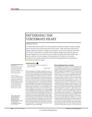
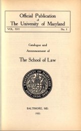
MalesAmer. Ind./Alask. Nat.BlacksMexican AmericansJapanese AmericansChinese AmericansPilipino AmericansPuerto RicansMajorityTABLE 2.1Delayed EducationRaw Measure a1960 1970 197645 C36410513144418352626041013261232232808NA d073910Social Indicator Values b(Ratios of raw measures tothe majority male population)1960 1970 19762.502.002.28.28.72.782.441.002.922.172.17.33.831.082.171.003.20*2.302.80.80NA .703.901.00FemalesAmer. Ind./Alask. Nat.BlacksMexican AmericansJapanese AmericansChinese AmericansPilipino AmericansPuerto RicansMajority4125330806032910231723010907240626152401NA 0327072.281.391.83.44.33.171.61.561.921.421.92.08.75.582.00.502.601.502.40.10NA .302.70.70a The percent of the 15-, 16-, and 17-year-olds who are 2 or more years behind the modal grade for their age. Specifically, thisis the proportion of the 15-, 16-, and 17-year-olds on April 1 who were in or below the 8th, 9th, and 10th grades, respectively.b See figure 2.1 for a graphic representation of the indicator values that appear in this table.c Bold type indicates that the difference between this value and the majority benchmark is statistically significant at the 0.10level. This means that if there were no difference between the groups in the entire population, samples of the size used herewould yield differences this large less than 10 percent of the time due to sampling error alone. See appendix C for data sourceand sampling information.d NA indicates that a value was not reported due to an insufficient sample size. Appendix C contains the sample size for allgroups and indicators.*This can be interpreted as follows: "In 1976 the delayed education rate for American Indian and Alaskan Native males was3.2 times greater than the rate of majority males."

Social Indicator Values: Ratios of rajiv measures to the majority male population.MalesAroer. Ind./AK Nat.196019701976Blacks196019701976Mexican Americans196019701976Japanese Americans196019701976Chinese Americans196019701976Plliplno Americans196019701976Puerto Rlcans196019701976Majority1960197019760.0FemalesAmer. Ind./AK Nat.196019701976Blacks196019701976Mexican Americans196019701976Japanese Americans196019701976Chinese Americans196019701976Filipino Americans196019701976Puerto Rlcans196019701976Majority196019701976EqualityEquality•Values were not available due to aj> insufficient number of cases.

In this study, a student is considered behind inschool if his or her grade is 2 years or more behindthe modal grade. 4 The measure of delay is calculatedfor persons 15 to 17 years old. These are the ages atwhich accumulated delays in the educational processcan be expected to be the longest and most evident.For these ages the 10th, 11th, and 12th grades aremodal, and those defined as behind in school are 15-year-olds in the 8th grade or less, 16-year-olds in the9th grade or less, and 17-year-olds in the 10th gradeor less. The delay rate is the percentage of those inthese categories out of all students of the same age.The percentages of those delayed in 1960, 1970, and1976 for both genders of every group discussed inthis report are contained in columns 1, 2, and 3 oftable 2.1.More than 40 percent of American Indian/AlaskanNative males and females, MexicanAmerican males, and Puerto Rican males were atleast 2 years behind the schooling progress for theirage in 1960. Although the delay rates have declinedfor these groups, in 1976, 25 percent or more ofAmerican Indian/Alaskan Native, Mexican American,and Puerto Rican males and females were still 2or more years behind the normal grade level for theirages. The delay rates reflect conditions that bothresult from and produce serious problems.Of even greater use are indicators that show howthe conditions measured are experienced in differentdegrees by different groups. All the indicatorspresented in this report have this characteristic and,therefore, provide meaningful measurements of agroup's degree of equality with the conditions ofmajority males, who serve as the reference group.Where possible, the differences between majoritymales and the other groups have been tested forstatistical significance using standard procedures, asdescribed in appendix C.The comparison of minorities' and women's ratesto the majority males' rate involves the calculation ofratios of the specific groups' measures to that of themajority males. The resulting numbers are relativemeasures with a clear interpretation such as, "In1976 the rate of delay of American Indian/AlaskanNative males was 3.2 times greater than that ofmajority males, while in 1960 it was only 2.5 timesgreater." The change in this ratio means that during4 For a similar use of modal grades, see U.S., Executive Office of thePresident, Office of Management and Budget, Social Indicators, 1973, table3/7, p. 102 (hereafter cited as Social Indicators, 1973 ).5 This figure of 2.1 percent represents an average decline over the decade of1.3 per year as a percentage of the estimated midyear figure of 38.5. Forthe 16-year period this group of males, compare r^tmajority males, became more likely to be delaym to nschool. The evidence underlying this statem isthat, although the delay rate for American i-an/Alaskan Native males decreased from 45 2from 1960 to 1976, this decrease (about 2.1 pe tper year) was too small to keep up with the rerapidly declining delay rate for majority males. 1elatter rate fell from 18 to 10 percent, or abo 6percent per year. 5 The ratios in figure 2.1 an mcolumns 4, 5, and 6 of table 2.1 indicate that mini ymales and females tend to have markedly hjjdelay rates than majority males. In fact, most o: eminority male groups experienced more than ethe delay rates of majority males, with Ame nIndian/Alaskan Native and Puerto Rican esexperiencing a delay rate in 1976 that was more nthree times that for majority males. Althoughdelay rates as a whole are lower than thos

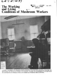
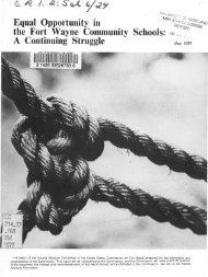
;ame incomes as those who complete their highICJPOI education. 6fe term "dropout" may be inappropriate for thisdeparture, since the implication is that theidual student took the initiative and "dropped|k of the educational system to spend his or herW at other, more highly valued activities. Some-)s the term "push-out" is more appropriate»use it focuses attention and responsibility on therool system itself for a student's failure to attain aP school education. 7 Regardless of why students^ot attend or finish high school, the consequences, if ever, desirable for either the individualsNation.nonattendance rate could signal a need for;cWective action. If nonattendance is concentratedr^prtain groups, then efforts to reduce nonattenecould be directed toward the needs of thoseps in order to deal most effectively with the)^Jlem. The second indicator in this series provideshak kind of information. As with the previousnro;ator, this one is based on 15- to 17-year-olds. Intl^case, the nonattendance indicator reflects thePOiientage of the high school age group that is notlied in school; the actual indicator is the ratio oftfl^ninority percentage to the majority percentage,information on nonattendance is contained in2.2 and figure 2.2.e indicator values show that minority groupnumbers are less likely than majority males to attendscWol during the important ages of 15 to 17.^Pough most groups have reduced their nonatteniamcQrates since 1960 and even since 1970, relative(^majority males many of the groups have notr^poved their likelihood of being in school. Fore^tfiple, in 1976 Mexican American females werenwe than twice as likely to be out of school asmales; this represented an increase of morethj| 40 percent over the 1970 ratio of the two groups.A^rerican Indian/Alaskan Native males and femaleslot noticeably reduce their nonattendance ratesbjg|een 1970 and 1976 while majority males reducednws by more than a third. Thus, the relativeAfrican Indian/Alaskan Native nonattendanceincreased appreciably. By 1976 AmericanInWan/Alaskan Native males were 2.80 times andAfrican Indian/Alaskan Native females 3.00 timesstopher Lasch, "Inequality and Education," in The "Inequality"CblWoversy, edited by Mary Jo Bane and Donald M. Levine (New York:Cooks, 1975), pp. 45-62."dren's Defense Fund, Children Out of School in America (Cambridge,* Children's Defense Fund, 1974), p. 17.as likely as majority males not to be enrolled in highschool.By itself, a high nonattendance rate damageschildren by limiting their exposure to academicinstruction; however, an additional and more devastatingspinoff is the negative influence on educationalattainment, which in turn tends to restrict lifelongsocial and economic standing. The remaining indicatorsof equality in this chapter measure suchconsequences of the disproportionate nonattendancerates of minorities and women.Educational AttainmentThe third indicator in this series extends the ideabehind the delayed education indicator and thenonattendance indicator to the issue of educationalattainment. Some very common categories used todistinguish different levels of attainment are "highschool diploma," "some college," and "4-year collegedegree." The social condition reflected in this idea ofattainment is the amount of time spent in formaleducation settings. As will be demonstrated later, thisinvestment of time in education is directly related tosubsequent levels of earnings and types of occupations.The amount of time spent in the educationalprocess has been expanding considerably for at leastas long as such statistics have been collected. Thepercentage of 17-year-olds who were high schoolgraduates was about 2 percent in 1870 and has grownsteadily to about 80 percent in the 1970s. 8 Inaddition to the increase in years of schooling, theschool year itself has expanded. About 34 additionaldays have been added to the usual school year sincethe start of this century. 9For the purposes of this study, the central issuehere is whether women and minority males achievethe same levels of educational attainment as majoritymales and, if not, whether the gap in educationalattainment between majority males and the rest ofsociety has increased or decreased. To measure this,two separate social indicators have been developedbased on high school completion and completion of4 or more years of college.Selecting the age group for measuring these twoeducational characteristics has important consequences.The more common technique has been to8 U.S., Department of Commerce, Bureau of the Census, HistoricalStatistics of the United States, Colonial Times to 1970, Bicentennial Edition,part 1(1975), p. 379.9 U.S., Department of Health, Education, and Welfare, Toward A Social9 9 6 5

MalesAmer. Ind./Alask. Nat.BlacksMexican AmericansJapanese AmericansChinese AmericansPilipino AmericansPuerto RicansMajorityFemalesAmer. Ind./Alask. Nat.BlacksMexican AmericansJapanese AmericansChinese AmericansPilipino AmericansPuerto RicansMajorityTABLE 2.2High School Nonattendance196029 C212602091225182423310314073012Raw Measure1970 19761516130606082609161517060909260814071102NA d06050515061401NA 101606Social Indicator Values b(Ratios of raw measures tothe majority male population)1960 1970 1976a The percent of 15-, 16-, and 17-year-olds who were not enrolled in school on April 1.b See figure 2.2 for a graphic representation of the indicator values that appear in this table.c Bold type indicates that the difference between this value and the majority benchmark is statistically significant at the 0.10level. See appendix C for sampling information and data source.d NA indicates that a value was not reported due to an insufficient sample size. Appendix C contains the sample size for allgroups and indicators.*This can be interpreted as follows: "In 1976 the high school nonattendance rate for American Indian and Alaskan Nativemales was 2.80 times greater than the rate for majority males."1.611.171.44.11.50.671.391.001.331.281.72.17.78.391.67.671.671.781.44.67.67.892.891.001.781.671.89.671.001.002.89.892.801.402.20.40NA1.201.001.003.001.202.80.20NA2.003.201.20

Social Indicator Values: Ratios of raw pleasures to the majority male population.Amer. Ind./AK Nat.196019701976Males o.o 1.0Blacks196019701976Mexican Americans196019701976Japanese Americans196019701976Chinese Americans196019701976Pilipino Americans196019701976Puerto Ricans196019701976Majority196019701976Females o.oAmer. Ind./AK Nat.196019701976Blacks196019701976Mexican Americans196019701976Japanese Americans196019701976Chinese Americans196019701976Pilipino Americans196019701976Puerto Ricans196019701976Majority1960197019761.0EqualityEquality"Values were not available due to an insufficient number of cases.

MalesAmer. Ind./Alask. Nat.BlacksMexican AmericansJapanese AmericansChinese AmericansPilipino AmericansPuerto RicansMajorityTABLE 2.3High School Completion196033 C41348984812469Raw Measure a1970 197658595594907744837074649888816887Social Indicator Values b(Ratios of raw measures tothe majority male population)1960 1970 1976.48.59.491.291.221.17.351.00.70.71.661.131.08.93.531.00.80*.85.741.131.01.93.781.00FemalesAmer. Ind./Alask. Nat.BlacksMexican AmericansJapanese AmericansChinese AmericansPilipino AmericansPuerto RicansMajority294235848276247056625194888442825874589990786086.42.61.511.221.191.10.351.01.67.75.611.131.061.01.51.99.67.85.671.141.03.90.69.99a The percentage of persons from 20 to 24 years of age who have completed 12 or more years of school.b See figure 2.3 for a graphic representation of the indicator values that appear in this table.c Bold type indicates that the difference between this value and the majority benchmark is statistically significant at the 0.10level. See appendix C for sampling information and data source.* This can be interpreted as follows: "In 1976 the high school completion rate for American Indian and Alaskan Native maleswas 80 percent of (or 20 percent below) the completion rate for majority males."

Social Indicator Values: Ratios of rawjmeasures to the majority male population.MalesAm*. Ind./AK Nat.196019701976Blacks196019701976Mexican Americans196019701976Japanese Americans• 196019701976Chinese Americans196019701976Pilipino Americans196019701976Puerto Ricans196019701976Majority1960197019761.6 FemalesAmer. Ind./AK Nat.196019701976Blacks196019701976Mexican Americans196019701976Japanese Americans196019701976Chinese Americans196019701976Pilipino Americans196019701976Puerto Ricans196019701976Majority196019701976Equality;Equality

MalesAmer. Ind./Alask. Nat.BlacksMexican AmericansJapanese AmericansChinese AmericansPilipino AmericansPuerto RicansMajorityFemalesAmer. Ind./Alask. Nat.BlacksMexican AmericansJapanese AmericansChinese AmericansPilipino AmericansPuerto RicansMajorityTABLE 2.4College Completion196003 c040435491904200206021326160109Raw Measure1970 197608 0806 1105 1139 5358 6028 3404 0622 3405 0408 1103 0531 3542 4450 5103 0414 22Social Indicator Values b(Ratios of raw measures tothe majority male population)1960 1970 1976.15.20.201.752.45.95.201.00.10.30.10.651.30.80.05.45.36.27.231.772.641.27.181.00.23.36.141.411.912.27.14.64.24*.32.321.561.761.00.181.00.12.32.151.031.291.50.12.65a The percentage of persons from 25 to 29 years of age who have completed at least 4 years of college.b See figure 2.4 for a graphic representation of the indicator values that appear in this table.c Bold type indicates that the difference between this value and the majority benchmark is statistically significant at the 0.10level. See appendix C for sampling information and data source.* This can be interpreted as follows: "In 1976 the college completion rate for American Indian and Alaskan Natives male was24 percent of (or 76 percent below) the rate for majority males."

Social Indicator Values: Ratios of raw measures to the majority male population.Amer. Ind./AK Nat.196019701976Males 3.0 2.25Blacks196019701976Mexican Americans196019701976Japanese Americans196019701976Chinese Americans196019701976Pilipino Americans196019701976Puerto Ricans196019701976Majority196019701976FemalesAmer. Ind./AK Nat.196019701976Blacks196019701976Mexican Americans196019701976Japanese Americans196019701976Chinese Americans196019701976Pilipino Americans196019701976Puerto Ricans196019701976Majority196019701976EqualityEquality

•base educational attainment statistics on persons 25years old and over, since they represent an age groupwhich, with few exceptions, has completed itsschooling. 10 Although that age range does provide agood basis for calculating trends for long timeperiods, for the particular purpose of measuringrecent trends it is not the most desirable. This isbecause a large part of the 25 years and over agegroup consists of persons who completed their,educations decades prior rather than participated inthe most recent changes in educational attainment.Furthermore, use of this large age group forcomparisons with majority males would tend toexaggerate the inequalities to the extent that recentchanges have been beneficial to minorities andwomen.A much more direct assessment of short-termtrends that does not overstate the extent of inequalitycan be obtained by limiting the analysis to the agegroup most likely to be just completing its educationand, therefore, to have experienced the latest changein educational attainment. Thus, high school completionrates are calculated here for 20-to-24-year-oldsin order to get a more accurate indication of thetrends. For the college attainment indicator, the agegroup selected is 25 to 29 years old. The completionrates and the social indicators for high school appearin table 2.3 and figure 2.3, while those for collegeattainment are contained in table 2.4 and figure 2.4.These tables show that at each point measured, theminority males' and females' levels of educationalattainment, with few exceptions, were substantiallybelow those of majority males. It is evident, inparticular, that, even by 1976, attainment of a collegeeducation was still far beyond the reach of almost allAmerican Indian/Alaskan Natives, blacks, MexicanAmericans, and Puerto Ricans.All of these groups showed improvements in theirrelative rates of high school completion except forthe Asian American populations, who declined orstayed the same in each case. While the AsianAmerican groups typically had higher rates of highschool completion at each time (1960, 1970, and1976), their relative educational advantage hasslipped because the majority male rate of high schoolcompletion has increased at a faster pace.In general, the minority male and female rates ofhigh school completion were about 65 to 85 percentof the rates for majority males in 1976. The college10Social Indicators, 1973; and U.S., Department of Commerce, Bureau ofthe Census, Statistical Abstract of the United States: 1974.completion rates, on the other hand, showgreater degree of disparity between majoritymajority females, and minority males and feExcept for the Asian American groups and majoroyfemales, the groups' rates do not even approachlplfthe college completion rates of majority males,majority females are still 35 percent less likelymajority males to have completed 4 or morecollege in 1976. In general, although JapChinese, and Pilipino Americans are more likelymajority males to complete a college education,relative advantage slipped somewhat from 191976.During the sixties, no group experienced a dein the percentage of those 25 to 29 years of agecompleted 4 or mpre years of college; however,was not the case from 1970 to 1976. More isome groups actually declined, relative tomales, in their rates of college attainment. gwith the Asian American populations menti(^pdabove, American Indian/Alaskan Native males jadfemales, black females, and Puerto Ricanwere relatively less likely to have completedin 1976 than in 1970.This draws attention to the fact that, althdalmost all groups have increased the percentagitheir populations having completed a college ed,tion, these increases do not match the increasemajority males. Thus, acknowledgment of ieducational attainment for minorities and WOmust be qualified with the observation thatremains a great amount of inequality of educSKattainment, and in some instances that inequalitieincreasing.^Indicators Based on the #Consequences of Education £The first three indicators could be describerelated to the quantity of education or the duraof the educational process. The next two indiare directed at the consequences of schoolingthe type of occupations people pursue andannual earnings, or the extent that minoritieswomen with educational attainment equal to ththe majority males are able to achieve equal refrom that training. As traditional educational balersare breached by minorities and women, thisof educational equality, based on the16

;orae consequences of educational attainment, becomesir^pasingly important. 11:upational Overqualificatione aspect of this type of educational equality canrased as follows: "For the same job, or for jobssimilar skill or educational requirements (suchositions requiring a college degree), mustties and women demonstrate greater skill oreducational accomplishments than majority" Where this type of discrimination exists,rriflfcrities and women must be educationally overqu^ifiedin order to obtain employment or promothoughthe census does not collect sufficientintormation on people's occupations to construct aniiwRator of occupational overqualification, it wasto supplement census data with otherin the construction of such an indicator.. Department of Labor's annual Occupational(MMook Handbook provides information on the1 educational requirements for specific occupa-As a result of careful examination and testingo4fc job-by-job basis by Commission staff, two typesofoccupational categories were selected as the basisfSRhe overqualification indicators: occupations thatilly require less than a high school diploma, ande that require less than a college degree,endix A contains the occupational categoriesthe corresponding educational requirements,measures of educational overqualification havedeveloped. The measure of high school overq^ificationis the percentage of high school gradu-" whose occupations typically do not require highol completion. The measure of college overqualionis the percentage who have completed ata year of college (13 or more years of education)'se occupation requires less education than that. 13overqualification indicators are the ratios ofpercentages of overqualified minorities andles to the percentage of overqualified majority; the calculation process is identical to those forratios previously presented. Tables 2.5 and 2.6figures 2.5 and 2.6 contain the high school andcdfcge overqualification measures and the derivedrSs for 1960, 1970, and 1976.nes S. Coleman, "Increasing Educational Opportunity: Researchms and Results," in The Condition for Educational Equality, edited byng M. McMurring (New York: Committee for Economic Developp.105.Department of Labor, Bureau of Labor Statistics, Occupationalk Handbook, 1974-75 Edition.The overqualification measures demonstrate thatoverqualification is prevalent among all groups andfor both educational levels measured. In fact, in1976, from 40 to 60 percent of high school graduateshad jobs that required less education. However, theseindicators also show that overqualification is moreprevalent among women and minority males thanmajority males. For example, black males with a highschool education are about 50 percent more likely tobe overqualified for their occupations than majoritymales. While all levels of high school overqualificationincreased from 1970 to 1976, the pattern of theindicator values (the ratios) is somewhat inconsistent,since some of the increases were more and some lessthan that for majority males.In a labor market where the match betweenpeople's qualifications and their jobs is not influencedby minority or gender status, it would beexpected that the different groups would have equaldegrees of overqualification. As it is, a disproportionatelyhigh number of minority persons surpass thetypically stated requirements for their occupations.The other side of the coin is that the majority malesin those occupations are much less likely to beoverqualified for those occupations. Apparently, amember of the majority male population with a highschool education is more likely to be able to obtain ajob that requires that level of education.The college overqualification pattern in table 2.6and figure 2.6 is not quite so clear. The same patternof disproportionate overqualification is evident forminority males, but the degree of disparity is not asgreat as for the high school indicator. Whereas blacksin 1976 were about 50 percent more likely to beoverqualified at the high school level, they wereabout 25 percent more likely to be overqualified atthe college level.The relatively greater equality of college overqualification,however, affects far fewer women andminority males than does the disproportionate highschool overqualification. For black males in 1976, forexample, seven times as many were in the "highschool completed" category as were in the "collegecompleted" category, which means that the progressdocumented in the college overqualification indicatorreflects changes in the conditions of only a small13 Of those who have completed 1 year or more of college, two sets ofindividuals are identified as overqualified: those whose occupation requiredonly high school or less, and those who had 4 years or more of college whoseoccupation required some college or less. A complete list of the occupationaltitles and their typical educational requirements can be found in appendixA.17

MalesAmer. Ind./Alask. Nat.BlacksMexican AmericansJapanese AmericansChinese AmericansPilipino AmericansPuerto RicansMajorityTABLE 2.5High School Overqualification196071.7°70.255.651.834.662.658.240.2Raw Measure 31970 197659.566.156.843.433.849.354.837.660.567.259.648.443.349.560.844.2Social Indicator Values b(Ratios of raw measures tothe majority male population)1960 1970 19761.781.751.381.29.861.561.451.001.581.761.511.15.901.311.461.001.371.521.351.10.981.121.381.00FemalesAmer. Ind./Alask. Nat.BlacksMexican AmericansJapanese AmericansChinese AmericansPilipino AmericansPuerto RicansMajority56.565.142.844.527.235.854.033.448.053.042.035.425.733.238.529.953.056.152.550.848.334.859.049.01.401.621.061.11.68.891.34.831.281.411.12.94.68.881.02.801.201.271.191.151.09.791.331.11a The percent of high school graduates who are employed in occupations which require less than a high school degree.b See figure 2.5 for a graphic representation of the indicator values that appear in this table.c Bold type indicates that the difference between this value and the majority benchmark is statistically significant at the 0.10level. See appendix C for sampling information and data source.*This can be interpreted as follows: "In 1976 the high school overqualification rate for American Indian and Alaskan Nativemales was 37 percent higher than (or 1.37 times) the rate for majority males."

catiSocial Indicator Values: Ratios of raw measures to the majority male population.MalesAmer. Ind./AK Nat.196019701976Blacks196019701976Mexican Americans196019701976Japanese Americans196019701976Chinese Americans196019701976Pilfpino Americans196019701976Puerto Rlcans196019701976Majority196019701976ooFemalesAmer. Ind./AK Nat.196019701976Blacks196019701976Mexican Americans196019701976Japanese Americans196019701976Chinese Americans196019701976Plliplno Americans196019701976Puerto Ricans196019701976Majority196019701976Equality

tooMalesAmer. Ind./Alask. Nat.BlacksMexican AmericansJapanese AmericansChinese AmericansPilipino AmericansPuerto RicansMajorityTABLE 2.6College OverqualificationRaw Measure 11960 1970 197651.658.846.952.448.248.152.942.749.2 C52.647.344.338.345.144.741.751.955.046.549.451.356.241.044.7Social Indicator Values b(Ratios of raw measures tothe majority male population)1960 1970 19761.211.381.101.231.131.131.241.001.181.261.131.06.921.081.071.001.161.231.041.101.151.26.921.00FemalesAmer. Ind./Alask. Nat.BlacksMexican AmericansJapanese AmericansChinese AmericansPilipino AmericansPuerto RicansMajority46.241.628.132.339.037.142.229.838.735.131.735.034.538.229.824.746.641.338.841.151.239.650.445.41.08.97.66.76.91.87.99.70.93.84.76.84.83.92.71.591.04.92.87.921.14.891.131.02a The percent of persons with at least 1 year of college who are employed in occupations which typically require less educathanthey have.b See figure 2.6 for a graphic representation of the indicator values that appear in this table.c Bold type indicates that the difference between this value and the majority benchmark is statistically significant at the 0.10level. See appendix C for sampling information and data source.* This can be interpreted as follows: "In 1976 the college overqualification rate for American Indian and Alaskan Native maleswas 16 percent higher than (or 1.16 times) the rate for majority males."

Social Indicator Values: Ratios of raw measures to the majority male population.MalesAmer. Ind./AK Nat.196019701976Blacks196019701976Mexican Americans196019701976Japanese Americans196019701976Chinese Americans196019701976Pllipino Americans196019701976Puerto Rlcans196019701976Majority196019701976.50 .75 Females .soAmer. Ind./AK Nat.196019701976Blacks196019701976Mexican Americans196019701976Japanese Americans196019701976Chinese Americans196019701976Pllipino Americans196019701976Puerto Ricans196019701976Majority196019701976Equality

portion of black males. In the much larger highschool category, the overqualification rate is 50percent greater than that for the majority males.One of the noteworthy points of this indicator isthe shift of relative overqualification for majorityfemales from 1970 to 1976. In 1970 majority femaleswere 41 percent less likely than majority males to beoverqualified in their occupations, but in 1976 theywere about as likely as the males to be overqualified.This change suggests that the increased labor forceparticipation of women 14 might have produced adiscriminatory side effect of limiting their participationto occupations that do not match their skills.Earnings for Educational LevelsStaying in school is often assumed to increase aperson's chances of getting better jobs and makingmore money. 15 Figure 2.7 displays the pattern of theaverage (median) earnings in 1975 for different levelsof educational attainment for black males andfemales and for majority males and females. Clearly,earnings tend to be higher for people with highereducational attainment. This is especially evident inthe substantial difference between those with highschool diplomas or some college and those with 4 ormore years of college.A basic question of equality is whether thefinancial rewards of schooling are equivalent forwomen, minorities, and majority men. Phrasednegatively, the question becomes, "Are the penaltiesfor dropping out of high school or college, or of notgoing to college, the same for women and minoritymales as they are for majority males?" The answer isdefinitely no. This disparity is graphically displayedin figure 2.7. It is evident that there are large earningsdifferences for black males and females and majorityfemales, compared with majority males, at eacheducational attainment level. In no educationalcategory do the female averages match the maleaverages. Majority female college graduates haveaverage earnings less than majority males with a highschool education. Although educational attainmentseems to be linked to earnings, people in differentgroups with the same educational attainment certainlydo not earn the same income. This indicator, inconjunction with the data on college attainment (see14 U.S., Department of Commerce, Bureau of the Census, CurrentPopulation Reports, A Statistical Portrait of Women in the United States(April 1976), Series P-23, no. 58, table 7-2, p. 28.15 Christopher Jencks, Inequality (New York: Basic Books, 1972), p. 221.16 The selection of this category for the indicator is somewhat arbitrary, but4 years of college seem to represent the clearest educational achievementtable 2.4), reflects a bleak picture for black ycmen and women and for majority women. Thfwho do overcome the obstacles to a collegetion find financial rewards significantly lower {those for majority males.Although figure 2.7 displays the pattern of (inequality of earnings by educational attain]quite well, it is important to have an indicatequantify this earnings inequality so patterns (time can be monitored. The indicator selecteethis purpose is the ratio of earnings figures forearning some income during the year and withmore years of college (i.e., the group supposed!most mobile, ready to reach equality, andsubject to disadvantages of limited schooling). 1

Earnings$16,000"Majority Males14,00012,000Black Males10,000Black Females8,000Majority Females6,000-4,000-2,000-1st-7th gradeEducation8th-11th grade 12th-15th grade 4 or more yrs.

MalesAmer. Ind./Alask. Nat.BlacksMexican AmericansJapanese AmericansChinese AmericansPilipino AmericansPuerto RicansMajorityFemalesAmer. Ind./Alask. Nat.BlacksMexican AmericansJapanese AmericansChinese AmericansPilipino AmericansPuerto RicansMajorityTABLE 2.7Earnings Differential for College-Educated Persons1959$44954482537652505589371340806833N.A. C27501382199948716674991739Raw Measure1969 1975$ 721077757848100459068779385441065131365855265221711875387522501943$116781232410786142531279013091N.A.151651028399116967838364219038N.A.8106Social Indicator Values"(Ratios of raw measures tothe majority male population)1959 1969 1975a Median earnings of those with 4 or more years of college who had some earnings during the year. This indicator is based onmedians and therefore standard techniques for estimating sampling error do not apply. See appendix C for data source andsampling information.b See figure 2.8 for a graphic representation of the indicator values that appear in this table.c NA indicates that a value was not reported due to an insufficient sample size. Appendix C contains the sample size for allgroups and indicators.*This can be interpreted as follows: "In 1975 American Indian and Alaskan Native males with 4 or more years of collegeearned 77 percent of the average for majority males with the same educational attainment.".66.66.79.77.82.54.601.00N.A..40.20.29.07.24.07.25.68.73.74.94.85.73.801.00.29.55.25.20.18.36.21.18.77.81.71.94.84.86N.A.1.00.68.65.46.55.42.60N.A..53

Social Indicator Values: Ratios of raw measures to the majority male population.MalesAmer. Ind./AK Nat.195919691975Blacks195919691975Mexican Americans195919691975Japanese Americans195919691975Chinese Americans195919691975Pilipino Americans195919691975Puerto Ricans195919691975Majority195919691975FemalesAmer. Ind./AK Nat.195919691975Blacks195919691975Mexican Americans195919691975Japanese Americans195919691975Chinese Americans195919691975Pilipino Americans195919691975Puerto Ricans195919691975Majority1959196919751.0N.A;-o.- 0.50• ','• 1 • • & AISwiiairW s0.25EqualityEqualityto'Values were not available due to an insufficient number of cases.

ConclusionThe indicators discussed in this chapter revealserious inequalities in education for minorities andwomen, compared to majority males. While the ideaof minority educational disadvantage certainly is notnew, these indicators provide greater detail on thespecific educational disadvantages of particularminority and gender groups than has been availablepreviously.In general, minority males and females havedecreased their delay and nonattendance rates overtime; however, their relative rates with respect tomajority males have not improved. In fact, mostminority males and females have greater relativedelay and nonattendance in 1976 than in either 1970or 1960, indicating a trend of increasing inequality.Among the personal and social consequences ofthese disparities is the fact that women and minoritymales fall far below majority males in their levels ofeducational attainment. As of 1976, among 25-to-29-year-olds, for every 100 majority males, 34 werecollege educated, while only about 11 out of 100minority males or minority females were collegeeducated. In other words, most minority and femalegroups remained only about 30 percent as likely asmajority males to have a college education.Although the Asian American groups do notexperience the same disparities in college attainment,their relative advantage is slipping over time. Inaddition, it is clear (and will be discussed further inchapter 4) that the greater educational attainment ofthe Asian American populations does not result inincreased financial rewards compared to majoritymales, as would be expected if everything else wereequal.Overall, the educational enrollment indicatorsverify the findings of many reports by the U.S.Commission on Civil Rights calling for renewedcommitment to equal educational opportunity. 18Two important issues concerning the college attainmentindicator deserve special mention. First, withoutcareful analysis, the rates of increased attainmentfor minorities and women may overshadow theinequalities that still persist. For example, MexicanAmerican and black males have almost tripled theirrates of college attainment during the 16-year period18 For example, the following publications have been issued by the U.S.Commission on Civil Rights: Racial Isolation in the Public Schools, 1967;The Mexican American Education Study, 6 vols., 1971-74; The Federal CivilRights Enforcement Effort—1974, Vol. Ill: To Ensure Equal EducationalOpportunity, 1975; Desegregating the Boston Public Schools: A Crisis in Civicreviewed. Both groups, however, also remained^rethan one-third as likely as majority males tocompleted 4 years of college in 1976.The second issue is that the relatively lowcollege attainment for women and minority1976 are occurring among the age groups mostto have been exposed recently to a college edtion—the population aged 25 to 29. Sinceyoung people are individuals who began elemenJjjvschool after the decision in Brown v. BoarcKfEducation, 19 this indicator reflects in part the £of continued unconstitutional discriminationaleducation.The indicators in this chapter go furthermerely providing numerical verification of enj|Umentdisparities, for they also show that the valuerpayoff of the struggle to attain an educa^i(measured in terms of occupation and earning^^ssignificantly less for most women and minority Senthan for majority males of the same educati^dlevel. For instance, the overqualification indicantsshow that majority males with high school edtions were more likely to find jobs that requiredlevel of education than were most femalesminority males. The race and gender disparitieslarger for high school overqualificationcollege overqualification—that is, the disparitworse at the level that affects far morealthough only 11 percent of black malesyears of college in 1976, 74 percent had complhigh school. Interestingly, majority females wihigh school diploma or some college were morethan majority males to find jobs requiringeducation in 1960 and in 1970, but by 1976 theybecome more educationally overqualified thanjority males.For those individuals who are able to fcollege—approximately 11 percent for minmales and females, 22 percent for majority femand 34 percent for majority males—the finapayoffs vary by ethnicity and sex. As indicate^^ifigure 2.7, black males and females and majmales and females certainly increasecollege graduates, although significant gapsthe groups occur at each attainment level. Inearnings differential for college-educated perindicates that even when women and minorityResponsibility, 1975; Fulfilling the Letter and Spirit of the Law, 19Twenty Years After Brown, 1977. Each was published by thGovernment Printing Office, Washington, D.C.19 Brown v. Board of Education, 347 U.S. 483 (1954).26

suWeed in completing a college education, they are males but, as college graduates, they earned far lesslii^r to earn far below what comparably-educated than majority males. Clearly the continuing severe;y males earn—approximately 85 percent for disparities between the earnings of women and menrn^rity males and less than 70 percent for minority at the same educational levels indicates the necessitymajority females. In 1976, Japanese, Chinese, for more vigorous efforts to ensure equal opportunityPilipino Americans were much more likely to j n employment,completed a college education than majority27

Chapter 3Unemployment and OccupationsBy almost any criterion, work is a vitally importantaspect of people's lives. For almost all persons, itrepresents a considerable investment of time andeffort. For minorities and women there is an addeddimension to the importance of work, since theyexperience some of the most damaging types ofdiscrimination and prejudice during their attempts tomake a living or pursue a career. Such discriminatorytreatment can touch every aspect of work—the typeof work a person is encouraged to prepare for, thelikelihood of finding work, the type of work done, thejob title and rank, the amount of pay, the extent towhich individual efforts are rewarded, the chancesfor advancement or of being laid off or fired, and ahost of other facets of work.The primary objective of this chapter is to developand promote the use of social indicators that will beuseful in measuring the reduction and elimination ofunjust hurdles and barriers to equal opportunity inthe world of work for minorities and women. Fourkey dimensions of work have been selected formeasurement: unemployment, occupational prestige,occupational mobility, and occupational segregation.Each represents a different aspect of the world ofwork in which women and minorities have criticalconcerns. Also, the educational overqualificationindicators presented in the previous chapter arebased on occupational characteristics and could havebeen included with these.1 U.S., Department of Labor, Bureau of Labor Statistics, "The EmploymentSituation," News (February 1977).2U.S., Department of Labor, Bureau of Labor Statistics, "Some SocialAspects of Unemployment," by Janet L. Norwood, Report 469, p. 1.;!The labor force is defined by the Bureau of the Census as includingpersons age 14 and older who either: (a) had worked during the week beforea census or population survey; (b) had a job from which they weretemporarily absent; (c) were looking for work during the past 4 weeks andwere available to accept a job; or (d) were waiting to be called back to a jobfrom which they had been laid off. These last two categories comprise the"unemployed," and the percentage of the labor force that is unemployed isUnemployment RateThe existence of a large number of willing and(potential workers without jobs has been a continMBgnational problem. Over 7 million persons in Srchquarter of 1976 were unemployed, and theirterm of unemployment was about 14 to 15 week1976, as has become typical, the likelihood of bland other races being out of work was aboutthat of whites. This type of disparity is the unemnjjpment indicator used in this report.^^The measurement of unemployment is ascated and controversial as it is important. "Uployment statistics represent people—people tto support families, people seeking their firstpeople changing jobs, people losing jobs." 2 Maecomplicated and controversial aspects of measurm: gemployment and unemployment involve the cnation of exactly which nonworking peoplebe classified as "unemployed."Persons not looking for work, but who wouldthey perceived some chance of being employed^rcnot listed as "unemployed," even though they n^egenerally experienced long periods of job ior have looked for work unsuccessfully. They areconsidered part of the "labor force" either. 3 Inst?they are called "discouraged workers," and aveevidence has shown a disproportionate numtthem to be women and minorities. 4 The cerhowever, did not seek the reason why people fail^look for work; therefore, it is impossible to deteroj^the "unemployment rate." Excluded from this definition of the laare persons whose "only activity consisted of work around thevolunteer work for religious, charitable, and similar organizat^u";students; retired workers; seasonal workers not currently looking for^Bk;disabled persons; inmates of institutions; and persons doing only u:—" Jwork in a family business for less than 15 hours in the preceding weefDepartment of Commerce, Bureau of the Census, Public UseBasic Records from the 1970 Census: Description and Technical Docuition (1972), p. 151.4 Paul O. Flaim, "Discouraged Workers and Changes in Unemploy:Monthly Labor Review, vol. 96, no. 3 (March 1973), p. 12.(28

number of persons who were not working in 1960F 1970 because they did not believe that theyfind jobs. As a result, this report is not able to[tribute statistical analyses involving differentlitions of the labor force and the unemployed,>ugh it is possible to convert standard unemployitrates to measures of inequality of unemployft.£}ie percentages of the various groups' labor forcestr^were defined as unemployed in 1960, 1970, andl!R are given in table 3.1. The exclusion ofcM^puraged workers from the unemployed categorypliably understates the unemployment rate ofrrSRmties and women more than it understates thatfi^najority males, since the discouraged workers areto be disproportionately minorities and wom-"hus, the disparities between the unemploymentof minorities and women in comparison tomales would also be understated,with the understatement, the disparitiesthe majority male rate of unemployment.the rates for majority females and for both sexesonerican Indians/Alaskan Natives, blacks, Mexic^Americans,and Puerto Ricans are generally verylajre. Although the unemployment rate fluctuatesCOTtinuously with changing economic conditions, thed^parities (ratios to the majority male rate oflployment) are more persistent and indicate ainequality in the labor market. The disparitychange only as the inequality is altered,jable 3.1 shows that most groups experiencedlines in their unemployment rates from 1960 tob; however, the ratios (see also figure 3.1) forindicate increases in disparities from the[prity male rate for black, Mexican American, andlino American men and for American Indi-(\laskan Native, black, and Mexican Americannen. This means that although the employmentition improved during the 1960s for these groups,pproved even more for majority males, and thee disparities continued.1 the period between 1970 and 1976, unemploy-|t rose for all of the groups discussed in this>rt. The majority male rate increased from 3.6 inb to 5.9 in 1976. During this period of risingLployment, the disparity between the minorityfemale rates and the majority male rate generallynley L. Friedlander, Unemployment in the Urban Core: An Analysis ofCities with Policy Recommendations (New York: Praeger Publishers,p. 122..., chapter 5.increased. Thus the unemployment of minorities andwomen worsened in absolute terms as well as relativeto majority males. Blacks, Puerto Ricans, andMexican Americans of both sexes moved fromhaving approximately twice the unemployment ofmajority males in 1970 to closer to three (and for onegroup, four) times the majority male rate in 1976.Consider the 1970-76 changes in the rates forblack males and females and Puerto Rican males andfemales. These four groups each experienced verysevere increases in unemployment relative to majoritymales. In each case the increase in the ratio wasgreater than 0.6 during the 6 years. This patternemphasizes the need for a two-pronged attack onunemployment. Policies to reduce unemploymentmust address both the absolute level of unemploymentand the level of disparities.One dramatic deviation from the pattern ofincreasing disparities is the case of AmericanIndian/Alaskan Native males, who had an extremelyhigh ratio of about 3.5 in 1960 (when the othergroups were closer to 2), but declined to 2.07 by1976, while other groups were moving in the oppositedirection. Thus, American Indian/Alaskan Nativemales experienced a significant improvement, butstill were more than twice as likely to be unemployedas majority males. Another notable reduction in theratios occurred for Pilipino American females. Theydeclined from an unemployment rate that was aboutfour times the majority male rate in 1960 to a levelclose to the majority male rate in 1976. Important asthese developments are for the groups involved, theycannot obscure the fact that the predominant trendfor most minorities and women is a worsening ofunemployment relative to majority males over time.One component of the unemployment rate warrantsseparate attention. Young women and minoritymen have the highest rates of unemployment of allgroups in the Nation. 5 In addition to its inherentproblems, the state of being unemployed seems to beassociated with activities and reactions on the part ofthe young that can be detrimental to themselves andto the communities in which they live. 6 The risk ofdeveloping frustrated and hostile youth who feelseparated from the society around them may beminimized by lowering the teenage unemploymentrate in areas of high unemployment. 77 U.S., Congress, Senate, Committee on Labor and Public Welfare,Subcommittee on Employment and Manpower, Toward Full Employment:Proposals for a Comprehensive Employment and Manpower Policy in theUnited States (1964), p. 67.29

u>oTABLE 3.1UnemploymentMalesAmer. Ind./Alask. Nat.BlacksMexican AmericansJapanese AmericansChinese AmericansPilipino AmericansPuerto RicansMajority196016.4 C8.68.12.43.64.98.84.7Raw Measure1970 197610.97.16.41.83.75.46.33.612.215.911.12.97.25.616.35.9Social Indicator Values b(Ratios of raw measures tothe majority male population)1960 1970 19763.491.831.72.51.771.041.871.003.031.971.78.501.031.501.751.002.072.691.88.491.22.952.761.00FemalesAmer. Ind./Alask. Nat.BlacksMexican AmericansJapanese AmericansChinese AmericansPilipino AmericansPuerto RicansMajority11.99.09.63.23.418.711.14.710.98.49.13.24.05.19.35.015.618.914.93.86.66.022.38.72.531.912.04.68.723.982.361.003.032.332.53.891.111.422.581.392.643.202.52.641.121.023.781.47a The percent of the labor force 15 years of age and older who were out of work and actively seeking work.b See figure 3.1 for a graphic representation of the indicator values that appear in this table.c Bold type indicates that the difference between this value and the majority benchmark is statistically significant at the 0.10level. See appendix C for sampling information and data source.*This can be interpreted as follows: "In 1976 the American Indian and Alaskan Native male unemployment rate was 2.07 timesas high as the rate of majority males."

Social Indicator Values: Ratios of raw measures to the majority male population.MalesAmer. Ind./AK Nat.196019701976Blacks196019701976Mexican Americans196019701976Japanese Americans196019701976Chinese Americans196019701976Pilipino Americans196019701976Puerto Rlcans196019701976Majority196019701976FemalesAmer. Ind./AK Nat.196019701976Blacks196019701976Mexican Americans196019701976Japanese Americans196019701976Chinese Americans196019701976Pilipino Americans196019701976Puerto Ricans196019701976Majority196019701976o.oEqualityEquality

MalesAmer. Ind./Alask. Nat.BlacksMexican AmericansJapanese AmericansChinese AmericansPilipino AmericansPuerto RicansMajority (teenage)Majority TotalFemalesAmer. Ind./Alask. Nat.BlacksMexican AmericansJapanese AmericansChinese AmericansPilipino AmericansPuerto RicansMajority (teenage)TABLE 3.2Teenage Unemployment196016.9 C12.114.47.0N.A. dN.A.14.89.84.720.918.812.58.6N.A.N.A.11.02.9Raw Measure 31970 197618.420.514.88.18.618.217.910.63.617.824.616.78.25.65.716.810.934.947.824.313.7N.A.22.155.215.05.936.051.327.19.9N.A.24.338.219.2Social Indicator Values b(Ratios of raw measures tothe majority male population)1960 1970 19763.602.573.061.49N.A.N.A.3.152.091.004.454.002.661.83N.A.N.A.2.34.625.115.704.112.252.395.064.972.941.004.946.834.642.281.561.584.673.035.92 :8.104.122.32N.A.3.759.362.541.006.108.694.591.68N.A.4.126.473.25a The percent of the labor force from 16 to 19 years of age who were out of work and actively seeking work.b See figure 3.2 for a graphic representation of the indicator values that appear in this table.c Bold type indicates that the difference between this value and majority benchmark is statistically significant at the 0.10 level.See appendix C for sampling information and data source.d NA indicates that a value was not available due to an insufficient sample size. Appendix C contains the sample size for allgroups and indicators.*This can be interpreted as follows: "In 1976 the American Indian and Alaskan Native male teenage unemployment rate was5.92 times the majority male total unemployment rate."

Social Indicator Values: Ratios of raw measures to the majority male population.Males 0.0Amer. Ind./AK Nat.196019701976Blacks196019701976Mexican Americans196019701976Japanese Americans196019701976Chinese Americans196019701976 "•*•HIPilipino Americans196019701976Puerto Ricans196019701976Majority (teenage)196019701976Majority Total1960197019762.5 10.0 FemalesAmer. Ind./AK Nat.196019701976Blacks196019701976Mexican Americans196019701976Japanese Americans196019701976Chinese Americans196019701976Pilipino Americans196019701976Puerto Ricans196019701976Majority (teenage)1960197019765.0 7.5 10.0•••*:^,. s * 1 - .•'!--"T -'-f-i^'Equality"Values were not available due to an Insufficient number of cases.Equality

Table 3.2 contains the teenage unemploymentrates for the various groups. The social indicator (seealso figure 3.2) compares the teenage rates to theoverall majority male rate. The rates for all thegroups are extremely high, and the minority andfemale groups are especially disadvantaged. Severalof the groups' teenage unemployment rates weremore than five times the rate of majority males in1970 and over eight times that reference point in1976. In virtually every case, the situation worsenedsubstantially during the decade of the 1960s and theneither continued to worsen or remained at anextremely high level in 1976. Unemployment forsome teenage groups reached a level in 1976 thatmeant that a third to one-half of the teenagers whowere actively seeking work were unable to find jobs.The approximate rates for these extremely hard-hitgroups were 35 percent for American Indian/AlaskanNative males, 48 percent for blackmales, 55 percent for Puerto Rican males, 36 percentfor American Indian/Alaskan Native females, 51percent for black females, and 38 percent for PuertoRican females.Occupational PrestigeIn addition to knowing how different the specificunemployment patterns of women and minoritymales are from that of majority males, it is importantto measure whether or not minorities and women aredisproportionately represented in occupations consideredless important, less prestigious, or lesssLloyd V. Temme, Occupation: Meanings and Measures (Washington, D.C.:Bureau of Social Science Research, 1975), p. 184.9 A commonly used wording in the interview situation is for the respondentto be asked:For each job mentioned, please pick out the statement that best givesyour own personal opinion of the general standing that such a jobhas: 1. Excellent standing, 2. Good standing, 3. Average standing, 4.Somewhat below average standing, 5. Poor standing; and category of"I don't know where to place that one."From Delbert Miller, Handbook of Research Design and Social Measurement(New York: David McKay Co., 1964), p. 173.Although it seems unlikely, it is logically possible that the actual types ofoccupations could be quite different even though the occupations are equalin prestige levels. In the scale used in this research, bank tellers andelectricians both have prestige scores of 44, and blasters, powdermen, andfile clerks have scores of 35.10 Temme, Occupation: Meanings and Measures .11 Ibid. The occupational title or category serves as the foundation formeasurement of many trends and characteristics of occupations. Thus,much of the variety of occupational activities and the significance of work isoversimplified and reduced to a category from the beginning. The categoriesare further accumulated to suit the needs of the researcher or agency untilthe desired degree of reduction of detail is accomplished.Although the Department of Labor's Dictionary of Occupational Titles nowcontains about 35,000 specific recognized and defined occupational titlesand thousands of new titles are being added (see U.S., Department ofLabor, Occupations Outlook Handbook, 1976-77 edition), the 1970 censusclassification of occupations contained only 441 occupational categories.The detailed 1970 census classification scheme required 137 pages of threeionadesirable by the rest of society. "Occupationalprestige" reflects the honor or social esteem gene^Pyaccorded to those working in an occupatk^8Measuring occupational prestige requires that numbersof the society evaluate occupationalin terms of relative "social standing." 9prestige scores can be calculated from numericalscores assigned to the evaluations of a large nui^;iof persons. This technique has yielded highly relive(i.e., consistent) prestige rankings of occupationalthe United States as well as in other countries. 10 %The prestige scores utilized here were ada|from a study that generated the scores foroccupational category used by the census. 11prestige scores range from a high of 88 for physicto a low of 1.5 for bootblacks. A few seleJoccupational prestige scores are listed inTwo different indicators have been devekfrom the prestige scores. Each is based on compsthe prestige scores of majority males towomen and minority males. The firstaverage prestige scores of the two groups b^compared, and the second measures the chaprestige for those who changed occupations betw«i1965 and 1970, and therefore describes mobility. Wislatter measure is based on a question asked foi1970 census but not asked in 1960 or 1976. AThe degree of inequality in the prestige scores^anbe clearly indicated by comparing themajority males to the means of the differentDividing a minority or female group's prestige scTTrecolumns each to list the occupations which comprise the 441 categorie^^eeU.S., Department of Commerce, Bureau of the Census, 1970Population, Classified Index of Occupations and Industries, 1971). Foi 1purposes the 441 categories are further reduced to 12 major catesprofessional, technical, and kindred workers; managers and administers,except farm; sales workers; clerical and kindred workers; craftsmen^nckindred workers; operatives, except transport; transport operatives; ^Brers,except farm; farmers and farm managers; farm laborers and rarrrforemen; service workers, except private household; and private houd"workers.For some purposes these 12 categories are further reduced to 4 (white iblue collar, service workers, and farmworkers). See, for example,'Department of Commerce, Bureau of the Census, Statistical Abstract AUnited States (1976), p. 360, table 581.iThe significance of the issue of classification and reduction goesconcern for detail. With the reduction of categories and the combinoccupations there is danger of misrepresenting the occupational situation.One possible result, for example, is that important differences i^fceoccupational structures of males and females are eliminated whe^^ieoccupations are combined. While it may appear that males and forteshave similar occupations, actually this "equality" is simply an artifaoHPaclassification system that combines divergent occupations.The "professional, technical, and kindred" category is an lmexample. Close examination of this category—which is often u:represent "high status occupations"—reveals a very diverse set oftions with widely varying duties, education, prestige, and income. Nairplane pilots, physicians, dancers, clergymen, recreation workers,therapy assistants, dieticians, and elementary school teachersincluded within the professional category.34

cupationTABLE 3.3Prestige Scores for Selected OccupationsPrestige Scorewyers 76fmentary School Teachers 64countants 61sdit Men 56rses 54cretaries 483ticians 47nk Tellers 44jctricians 44emen 41lletes 39rpenters 39Jesmen and Sales Clerks 38tomobile Mechanics 37asters and Powdermen 35e Clerks 35rm Foremen 33wers 29jck Drivers 29ne Operatives 27liters 24nitors 23iids 11irbage Collectors 11rm Laborers 10iurce: Lloyd V. Temme, Occupation: Meanings and Measures (Washjton,D.C.: Bureau of Social Science Research 1975), pp. 270-334.i35

MalesAmer. Ind./Alask. Nat.BlacksMexican AmericansJapanese AmericansChinese AmericansPilipino AmericansPuerto RicansMajority196025.7 C25.926.436.239.227.628.837.1TABLE 3.4Occupational PrestigeRaw Measure1970 197630.829.629.839.541.533.831.238.933.930.530.440.843.937.032.139.5Social Indicator Values b(Ratios of raw measures tothe majority male population)1960 1970 1976.69.70.71.981.06.74.781.00.79.76.771.021.07.87.801.00.86.77.771.031.11.94.811.00FemalesAmer. Ind./Alask. Nat.BlacksMexican AmericansJapanese AmericansChinese AmericansPilipino AmericansPuerto RicansMajority27.725.528.934.637.534.631.038.032.329.629.837.539.239.833.938.833.532.030.036.138.340.332.938.8.75.69.78.931.01.93.841.02.83.76.77.961.011.02.871.00.85.81.76.91.971.02.83.98a Mean Occupational Prestige Value.b See figure 3.3 for a graphic representation of the indicator values that appear in this table.c Bold type indicates that the difference between this value and the majority benchmark is statistically significant at the 0.10level. See appendix C for sampling information and data source.*This can be interpreted as follows: "In 1976, on the average, the prestige values of American Indian and Alaskan Nativemales' occupations were 86 percent of the average prestige values for majority males."

Social Indicator Values: Ratios of raw measures to the majority male population.MalesAmer. Ind./AK Nat.196019701976Blacks196019701976Mexican Americans196019701976Japanese Americans196019701976Chinese Americans196019701976Pllipino Americans196019701976Puerto Ricans196019701976Majority196019701976FemalesAmer. Ind./AK Nat.196019701976Blacks196019701976Mexican Americans196019701976Japanese Americans196019701976Chinese Americans196019701976Pllipino Americans196019701976Puerto Ricans196019701976Majority196019701976EqualityEquality

y the majority male average prestige score yields theproportion of the majority score that is attained bythe women or minority men.As with the previous indicators, a ratio of 1.0would indicate the averages are equal, and a ratio of0.6 would indicate that the minority or femalegroup's average is 0.6 (or 60 percent) of the majoritymale score. Thus, the indicator directly represents theextent of disparity between the two groups' averages.Table 3.4 contains the averages and ratios for 1960,1970, and 1976.The prestige indicator values in table 3.4 andfigure 3.3 show that blacks, American Indians/AlaskanNatives, Mexican Americans, andPuerto Ricans of both sexes typically have much lessprestigious occupations than majority males. Bygender, the scores are virtually identical for themajority group and very similar within most of theminority groups.The high concentration of women in a fewoccupations with relatively high prestige scores, suchas secretaries and other white collar occupations,contributes to the high average prestige scores forfemales. 12 Other indicators in this report emphasizemany significant differences in the occupations ofmales and females. Therefore, this similarity inoccupational prestige scores of men and womenshould be interpreted cautiously. An indicator laterin this chapter deals specifically with the extent towhich women and minority males have occupationssimilar to majority males.None of the minority male groups shows adecrease in average prestige scores relative tomajority males. Although the changes are not verylarge and major discrepancies clearly exist, it seemsthat the trend is for minority males to be moving intomore prestigious occupations at a slow pace, but,nonetheless, at a faster rate than majority males.While the average prestige score of majority malesincreased about one percentage point during eachinterval, the other male groups' average scoresincreased more substantially. Despite more rapidmovement toward more prestigious jobs, most12 In 1973 nearly two-fifths of all women workers worked as secretaries,retail trade salesworkers, bookkeepers, private household workers, elementaryschool teachers, waitresses, typists, cashiers, sewers and stitchers, andregistered nurses. U.S., Department of Labor, Employment StandardsAdministration, Women's Bureau, 7975 Handbook on Women Workers,Bulletin 197, p. 91.13 It has been estimated, however, that it will take approximately sevengenerations for blacks and whites to have similar occupational distributions,even if discrimination were to stop immediately. See Stanley Lieberson andGlenn V. Fuguitt, "Negro-White Occupational Differences in the Absenceof Discrimination," American Journal of Sociology, vol. 73, no. 2 (September1967), pp. 188-200.eMeminority male groups still have much lower presscores than majority males.The female groups show a far different patjAlthough each minority male group had its lowestindicator value of the time series in 1960 ^highest in 1976, among the female groupsfollowing had their worst scores in 1976: MeAmerican, Puerto Rican, and majority. From1976 one of the female groups' average pregicescores actually dropped in absolute as well as relatevalues, and one group's score remained the s(Q)e.Clearly, the female groups are still in a precaaapsituation without any encouraging trend. ^Occupational MobilityDisparity of occupational prestige levels bgroups can change through two processes,persons entering the labor force may be acinto occupations that earlier either did not exiwere closed to members of their race, ethnicor sex. Through this process, successive generaof women and minority men may becomesimilar to majority males in prestige levels M&

:fflmge that do not in fact indicate upward mobilityies for improvement.cause of this inadequacy, the indicator ofpational mobility used here is based on thechange in prestige scores of those whooccupations in the past 5 years. This changeto an occupation with a similar prestige scorea higher or lower score. The indicator itself isr^ratio of the average change for minorities andvoTnen to the average change for majority males.T^tadvantages discussed earlier of using ratios alsotto this indicator.the 1960 census and in the Survey of IncomeEducation in 1976, people were not asked totheir occupation 5 years earlier, so this indicatorol DfTc Occupational mobility is only available from thecensus; that is, for the 1965 to 1970 period. ThelnMsator values are contained in figure 3.4 and in3.5, which also includes the average change inge scores for those who changed occupations,w of the differences between the majority malesanjL the other groups are large enough to bestatically significant. The primary statistical reasonhis is the large variation in change scores thatbe observed in table C-2 in appendix C. Thecan American males show substantial relativebut the Mexican American, Chinese American,Pilipino American females all are far belowrity males. It should be recalled from theItous indicator that the absolute level of prestigeinority and female groups in 1970 was stilllower than for majority males, despite thed mobility of some of those who changedpupations.Occupational Segregation^ie critical issue of whether individuals in differhavedifferent occupations serves as theco«eptual basis for the next indicator of equality.Wrereas occupational characteristics were used forus indicators—i.e., prestige scores and educarequirementsassociated with specific occupa-—here the concern is more basic. The occupathemselvesare to be compared.occupational categories are described in note 11 above.«:, for example, Lieberson and Fuguitt, "Negro-White Occupationalfences in the Absence of Discrimination"; Reynolds Farley, "Trendscial Inequality: Have the Gains of the 1960's Disappeared in the'," American Sociological Review, vol. 42, no. 2 (April 1977), pp. 189-d Francine D. Blau, Equal Pay in the Office (Lexington, MassachuxingtonBooks, 1977).The term "segregation" reflects the extreme degreeof separation of races, ethnic groups, or sexes thatcan result from deliberate acts channeling andrestricting choices and opportunities. This phenomenoncan occur in the work place as well as inneighborhoods and schools. Two major types ofsegregation can be found in the world of work.Employment segregation implies that women andminorities have different employers than majoritymales, so that work settings are segregated. Occupationalsegregation refers to the situation in whichminorities and women have different occupations ortypes of jobs regardless of where or for whom theywork. In a hospital setting, for example, a majoritymale typically is a doctor, a woman is a nurse, and aminority male is an orderly. This type of extremeseparation of employees may be found in a variety ofindustries and appears to have been even morecommon in the past. Within the recent past, thelistings of job openings in newspapers were segregatedwith a section for males and one for females.Thus, segregation of occupations restricts women,minority males, and even majority males from fulland fair access to the available positions in the labormarket.The occupational segregation indicator, usingcomparisons to majority male occupations, allowsmeasurement of the degree to which occupationalsegregation exists and has changed in the recent pastfor minorities and women. This indicator, like theprevious two based on occupational prestige, requiresa classification of jobs. The classificationscheme used in this report is the most detailed thatthe Bureau of the Census offers, consisting of 441categories of occupations. 16To measure occupational segregation, the statisticaltechnique called the "index of dissimilarity" wasutilized. This index is a summary measure of theoverall differences between two percentage distributions.It has received wide use by others to measureoccupational differences, 17 as well as residentialsegregation 18 and other types of differences. Althoughpreviously the index of dissimilarity hastypically been used with the 12 major categories, it is18 Karl E. Taeuber and Alma F. Taeuber, Negroes in Cities: ResidentialSegregation and Neighborhood Changes (Chicago: Aldine, 1965); Thomas L.Van Valey, Wade Clark Roof, and Jerome E. Wilcox, "Trends inResidential Segregation: 1960-1970," American Journal of Sociology, vol. 82,no. 4 (January 1977), pp. 826-44; and Leslie Hollingsworth, Jr., "Indexes ofRacial Residential Segregation for 109 Cities in the United States, 1940 to1970," Sociological Focus, vol. 8, no. 2 (April 1975), pp. 125-42.39

MalesAmer. Ind./Alask. Nat.BlacksMexican AmericansJapanese AmericansChinese AmericansPilipino AmericansPuerto RicansMajorityFemalesAmer. Ind./Alask. Nat.BlacksMexican AmericansJapanese AmericansChinese AmericansPilipino AmericansPuerto RicansMajorityTABLE 3.5Occupational MobilityRaw Measure a1965-19701.852.402.73 C2.75.71-.132.121.92.891.88.56.34-3.45-3.78.781.37Social Indicator Values b(Ratios of raw measuresto the majority male population)1965-1970.96*1.251.421.43.37-.071.101.00.46.98.29.17-1.80-1.97.41.71a The average change in prestige scores for those who changed occupations between 1965 and1970.b See figure 3.4 for a graphic representation of the indicator values that appear in this table.c Bold type indicates that the difference between this value and the majority benchmark is statisticallysignificant at the 0.10 level. See appenddix C for sampling information and data source.*This can be interpreted as follows: "In 1970 the American Indian and Alaskan Native maleswho had different occupations in 1965 had, on the average, increased their occupational prestige96 percent of the majority male average increase."

Social Indicator Values: Ratios of rawjmeasures to the majority male.Males 2.0Amer. Ind./AK Nat.1965-1970Blacks1965-1970Mexican Americans1965-1970Japanese Americans1965-1970Chinese Americans1965-1970Plllpino Americans1965-1970' Puerto Ricans1965-1970Majority1965-1970-2.0 Females 2.0Amer. Ind./AK Nat.1965-1970Blacks1965-1970Mexican Americans1965-1970Japanese Americans1965-1970Chinese Americans1965-1970Plllplno Americans1965-1970Puerto Ricans1965-1970Majority1965-1970-1.0 -2.0Equality

MalesAmer. Ind./Alask. Nat.BlacksMexican AmericansJapanese AmericansChinese AmericansPilipino AmericansPuerto RicansTABLE 3.6Occupational Segregation aCompared with Majority MalesCompared with Majority Females1960 1970 1976 1960 1970 197644.144.736.728.950.650.749.238.244.336.631.352.246.044.135.7*37.938.241.561.459.750.4FemalesAmer. Ind./Alask. Nat.BlacksMexican AmericansJapanese AmericansChinese AmericansPilipino AmericansPuerto RicansMajority69.172.463.563.871.869.071.662.470.771.168.368.970.973.070.965.869.469.375.172.179.779.278.966.147.152.431.026.636.440.953.9—31.540.427.522.534.142.237.7—33.8**35.836.932.652.948.348.3——a Standard tests of statistical significance do not apply to this indicator. If, however, the indicatorvalue is viewed as a normal percentage, every percentage value presented in the table is significantlydifferent from 0.0, which is the reference point for equality for this indicator. See appendixC for sampling information and data source. See figure 3.5 for a graphic representationof the indicator values that appear in this table.*This can be interpreted as follows: "In 1976, at least 35.7 percent of American Indian andAlaskan Native males would have had to change occupations in order to have an occupationaldistribution identical to the majority males."**This can be interpreted as follows: "In 1976, at least 33.8 percent of American Indian and AlaskanNative females would have had to change occupations in order to have an occupationaldistribution identical to the majority females."

Compared with majority males.! MalesAmer. Ihd./AK Nat.1960i 19701976Blacks196019701976Mexican Americans196019701976Japanese Americans196019701976Chinese Americans196019701976PlllpEno Americans1960• 19701976; Puerto Ricans196019701976Majority196019701976100% Females oAmer. Ind./AK Nat.196019701976Blacks196019701976Mexican Americans196019701976Japanese Americans196019701976Chinese Americans196019701976Plliplno Americans196019701976Puerto Ricans196019701976Majority19601970197625% 50% 75% 100%EqualityEquality

even more useful and valid with a larger number ofcategories, such as the 441 used here.The index is simply calculated and easily interpreted.19 It represents the percentage of a group whowould have to change occupations in order for thegroup to have the identical occupational distributionof a comparison group. If two groups had the samedistributions of occupations, the index of dissimilaritywould be 0.0 (zero). For example, from the valuesfor the occupational segregation indicator presentedin table 3.6 and figure 3.5 the reader can see that 37.9percent of black males in 1976 would have had tochange their occupations in order for their group tobe employed in the same occupations in the sameproportions as the majority males.Table 3.6 and figure 3.5 show generally greatersegregation from 1960 to 1976 for women andminority males relative to majority males. This resultbecomes more significant when one considers thatduring this period an extensive occupational changetook place for women and minority men. 20 Thus,although minorities and women changed occupations,they still did not move proportionately into thetypes of employment held by the majority malepopulation. In 1976, five of the seven minority malegroups exhibited greater dissimilarity than in either1960 or 1970. Mexican American, Japanese American,Chinese American, Pilipino American, andPuerto Rican males all share this characteristic ofhaving their greatest segregation at the most recenttime—indicating that things clearly are not gettingbetter. 21At each time period, approximately three-fourthsof each female minority group would have had to19Given two percentage distributions (one for each group, and eachtotaling 100 percent) covering the same occupations, the percentage of onegroup in each occupation is subtracted from the percentage of the othergroup in that occupation. The sum of the percentage differences (disregardingthe sign) for all occupations is divided by two and the result is the indexof dissimilarity. See U.S., Department of Commerce, Bureau of the Census,Methods and Materials of Demography, second printing (rev.), by Henry S.Shryock, Jacob S. Siegel, and Associates (Washington, D.C.: U.S. GovernmentPrinting Office, 1974), vol. 1, pp. 232-33.20For example, our analysis of the 1970 census records used in this studyreveals that 44 percent of Mexican American males and 40 percent ofMexican American females between the ages of 25 and 64 changedoccupations between 1965 and 1970. These percentages refer only to thoseemployed in both 1965 and 1970. Moreover, the number of workers in sometraditionally minority and female categories such as "farmworkers, wageworkers" and "private household workers" sharply declined over the 1960decade. (Comparable information for 1976 was not available.)21It could be argued that the increasing dissimilarity should not beinterpreted as an unfavorable trend if the occupational change of one groupis to better jobs concentrated in a single industry. A group may becomehighly overrepresented among doctors and nurses, for example. Thenegative aspect to the increasing dissimilarity, even if everyone from onegroup went into medicine or some other field many regard as prestigious, isthat the process probably represents a continuing pattern of restricted freechange occupations to have a group occupati tiWalstructure resembling that of the majority males.^fle •Wiesegregation indicator actually increased from 19tifeto1970 (meaning the structure became more dissii^mrfrom majority males) for all groups except those ^Rohad experienced the greatest initial segregatioJ^n1960 (blacks, Puerto Ricans, and Chinese Americans),wThe dissimilarity scores were higher in 1976 Anin the other years for majority females and for tathsexes of Mexican Americans, Japanese Ameri

some groups, the dissimilarity was over 50pIPent. The figures indicate major shifts in somemjtority female occupational distributions. Forpie, black females moved more than 16 percentpointscloser to the majority female patternfrom 52.4 in 1960 to 40.4 in 1970 to 35.8 in1^^), while American Indian/Alaskan Native femrRsbecame 13.3 percentage points closer. As withtl^Jbther sets of scores, here, too, most of the groupshak their worst segregation in 1976. Clearly, thed^-epancies remain and the major trends are nottoBIrd a reduction in those discrepancies. Without ad^JDt, the gender occupational boundaries are mored^nct than are the racial-ethnic ones, though bothaf^learly present.^pie males and females of each minority grouph^| somewhat similar levels of dissimilarity fromtn^majority group of the same sex. In 1976, fore^mple, the American Indian/Alaskan Nativen^ks' occupations were 35.7 percent different frommajority males, and the American Indi-Native females were 33.8 percent differmajorityfemales. The comparable valuesales and females, respectively, are approximateand36 percent for blacks, 38 and 37 percent forAmericans, and 50 and 48 percent forRicans. The values are less similar fornese Americans, Chinese Americans, and Pilipimericans,but still the males and females aret^in about 10 percentage points.#e following generalized patterns are indicatede occupational segregation indicators calculatedi^^ure 3.5 and table 3.6:S^Occupational segregation has increased substanallysince 1970 for most of the groups studied inlis report. The pattern was mixed from 1960 toS70, with many groups showing almost noange, but a new trend seems to be operating.Approximately one-third to well over one-half of^e minority males would have had to change theircupations for their groups' occupational patternsf coincide with that of majority males in 1976.^^The highest degree of occupational dissimilarityS(n be found between the female groups andajority males. As noted previously, two-thirds toree-fourths of women's occupations in 1976have had to be changed to match the^rccupational patterns of the majority males.ConclusionThe indicators in this chapter measure importantelements of inequality in the world of work. Theunemployment indicator showed that minorities andwomen were much more likely than majority men tobe unemployed. Indeed, many of the groups werebetween two and four times as likely as majoritymales to be out of work. For most groups, thedisparity in unemployment grew worse during the1960s through 1976.Teenage women and minority males fared evenless well in finding jobs. Their rates of unemploymentwere generally from three to nine times higherthan majority males; the rate was over eight timeshigher for teenage blacks of both sexes and PuertoRican males. Again, a worsening of the relativeunemployment between the majority and othergroups occurred during the period analyzed.While the segregation indicator was concernedwith the size of the differences in the occupationaldistributions of minorities, females, and majoritymales, the prestige indicator showed that the socialesteem of the occupations of minorities and femaleswas also less than that of majority males. This factsuggests that not only are the jobs women andminorities have different, but the jobs are also valuedless by society in general. Although some meager,but consistent, improvement was observed for theminority males, the pattern for females was mixed.Approximately 40 percent of the minority andfemale populations changed occupations between1965 and 1970, indicating at least some possibility forimprovement in the types of occupation for minoritiesand females in comparison to the majority males.However, when the occupations were measured interms of the prestige values attached to the old andnew occupations, it was evident that minorities andfemales were less upwardly mobile than majoritymales. In fact, for some of the minority and femalegroups, the new occupation typically meant a declinein prestige over the old occupation.Minorities and females are segregated from themajority in the types of occupations they have. Atleast one-third of the minority males and two-thirdsto three-fourths of the minority females would haveto change their occupations in order for their groupsto have occupational distributions similar to themajority males. The time period analyzed saw noimprovement in the degree of segregation in occupationsbetween minorities and females in comparison45

to majority males. In fact, the degree of segregationbecame worse for Mexican American males andfemales, Japanese American males and females,Chinese American males and females, PiliAmerican males and females, and majority fe46

#(Mipter 4Income and Povertybased on money, such as median family!ome and real personal income, are probably usedPe than any other general kind of measure inlpts to represent how good or bad things are forPopulation or a segment of a population.Fsing income as an indicator of well-being seemsappropriate, and the use of money (dollars)Jiild not be interpreted as a diversion from theIctive of this report. Since the focus here is on thefibution of income among groups and the living[ditions of people with certain amounts of income,ler than with the general state of the economy, theistics derived are social indicators and notlomic indicators.lile not everyone equates money with wellquitea number of studies have noted therelationship between the amount of income and aTe of personal well-being. 1 The U.S. Departmentq^Health, Education, and Welfare study, Toward aial Report, which was a major impetus to theblopment of social indicator research, reported'income is a rough but convenient measure ofgoods and services—food, clothing, entertainft,medical care, and so forth—available to aor family or a nation." 2 Levels of well-beinglealth, housing, recreation, and consumption wereted to income levels in the 1975 Handbook onWorkers, 3 and the following profiles of thelevels were reported:lealth. In 1970 only 39 percent of families with}comes under $3,000 and 53 percent of familiesincomes between $3,000 and $5,000 had>spital insurance coverage; 84 percent of familiesincomes between $7,000 and $10,000 and 90PRainwater, What Money Buys: Inequality and the Social Meanings of(New York: Basic Books, 1974), p. 20.' Department of Health, Education, and Welfare, Toward a Social. 41.Department of Labor, Employment Standards Administration,percent of those with incomes over $10,000 hadcoverage.Housing. Of the 4.7 million substandard dwellingunits in the Nation, over half were occupied byfamilies with incomes less than $4,000 in 1970;only about one-tenth were occupied by familieswith $10,000 or more in income.Recreation. Households with incomes in 1970 of$7,500 to $9,999 spent more than twice as muchtime swimming, playing outdoor games or sports,bicycling, or camping as did those with incomesbelow $5,000.Consumer expenditures. The percentage of after-taxincome spent on living necessities such as housing,food, and transportation is proportionately greaterfor the lower than for higher income groups.During inflationary periods, expenditures for suchpurposes become particularly burdensome to lowincomegroups as they struggle to keep pace withrising living costs.In addition to buying food, shelter, clothing, andtransportation, money allows an individual to jointhe rest of society or of his or her ethnic or racialgroup in routine social, recreational, and entertainmentactivities. Thus, "money buys membership inindustrial soceity," 4 and in great part determineswhether an individual has a sense of belonging orone of alienation. More important, and oversimplifyinga complex social-psychological process, moneyallows for a wide range of activities that may"validate" a person's sense of self-worth and wellbeing.5Of the many aspects of income that are importantto all people, four issues are particularly vital toWomen's Bureau, 7975 Handbook of Women Workers, Bulletin 297, p. 143-44.4 Rainwater, What Money Buys, p. xi.5Ibid.47

minorities and women, and these provide the basisfor the indicators developed in this chapter. Theseissues are income equality, earnings equity, incomemobility (the "income ladder"), and poverty. In therecent past these issues have been focal points ofconcern with regard to the conditions of women andminorities.Equality of IncomeEquality of income among social groups is one ofthe major topics in social, political, and economicthought. The primary concern in discussion ofincome equality is generally with the unequaldistribution of income within a population. In theUnited States, and many other countries, a fewpersons receive a very large proportion of the incomeand a large proportion of the people receive a smallproportion of the income. At one end of the scale,since 1947, 20 percent of the Nation's families havehad to make do with only about 5 percent of the totalnational family income; at the other end, 5 percent offamilies have received about 16 percent of the totalnational family income. 6 If income were distributedmore equally, the top 5 percent would receive closerto 5 percent of the total income and the bottom 20percent would receive closer to 20 percent of the totalincome. In the United States, clearly, there is adisproportionate concentration of total income in asmall number of families, and there has beenvirtually no change in this pattern of inequality in thepast three decades.Here, the primary concern in the discussion ofincome equality is whether the distribution of thenational income among different groups (races,sexes, etc.) in our society is similar. In other words,when studying the overall distribution of income,analysts should also ask whether the distributionfollows group lines.Measuring "Average" IncomeOne way to answer the question just posed is tocompare the "average" incomes available to membersof different groups. For example, table 4.16U.S., Department of Commerce, Bureau of the Census, Statistical Abstractof the United States: 1974, p. 384, and Statistical Abstract of the UnitedStates: 1976, p. 406.7 U.S., Department of Commerce, Bureau of the Census, 1970 Census ofPopulation, vol. 1, Characteristics of the Population, Part 1, United StatesSummary, section 1, table 54, pp. 1-279-1-280.8 The percentage of the white population over 14 who received someincome for 1969 was 91 percent for males and 64 percent for females. Forthe black population, trie percentages are 88 percent for males and 72percent for females. U.S., Department of Commerce, Bureau of the Census,provides figures from published reports on Wmedian (a form of average) family income of wl^^and of blacks and other races from 1950 to 1976. W^income figures demonstrate a high degree of incominequality: blacks and other races received incoij^amounting to less than two-thirds of white fanfljincome during this period.^Social indicators for income equality can ha^Pform similar to indicators in previous chaptersaverage minority income divided by an avermajority income. For example, the ratios in tabindicate that during most of the 1960s, a period wvarious economic and social reforms were instituminority incomes scarcely improved relativemajority incomes; over a period of 24 years, theof minority to majority incomes rose onlyfrom 0.54 in 1950 to 0.63 in 1976.On the face of it, the "average income" of a grmay seem to be an ideal social indicator representhe income of that group. It is easy to compute,people can readily understand its meaning.some of the most common ways of calculaaverage incomes are not very suitable formeasurement of equality of income:• The median family income presented in tablefor example, is based only on those personsare living in a family situation (i.e., with aand thus excludes many of each group or population.Even as a measure of economic well-being^R*family units, the median family income isfor comparisions between different groups beethe typical size of the "average family consution unit" represented in the income statisticvary from group to group. To the extentminority groups have larger families, 7 the uthe median family income for comparisons ominority groups with the majority undersincome inequality for individuals.• Average personal income is a statisticrepresents people without regard to their fastatus, but it typically is based only on thosehave received some income during the yearthus excludes a sizable portion of the1970 Census of Population, vol. 1, Characteristics of the Population, PG^United States Summary, section 2, table 245.^These figures show that a sizable proportion of the population is^represented by income averages based on the above definition. Thej(show that the proportion varies between sexes and minority groups.Included in this group who received "some income" are part-time wo^full-time workers, part-year workers, and persons who only receivedsecurity and other benefits.It seems clear that a statistic such as the average income for those withincome is based on so many divergent types of income that it would JaKe48

TABLE 4.1Median Income of Families: 1950 to 1976Black andother races$1,8692,0322,3382,4612,4102,5492,6282,7642,7113,1613,2333,1913,3303,4653,8393,9944,6745,0945,5906,191Race of HeadWhite$ 3,4453,8594,1144,3924,3394,6054,9935,1665,3005,8935,8355,9816,2376,5486,8587,2517,7928,2348,9379,794Ratio:Black andother racesto white0.540.530.570.560.560.550.530.540.510.540.550.530.530.530.560.550.600.620.630.636,5166,7147,1067,5968,2659,3219,82110,23610,67211,54912,59513,35614,26815,5370.640.630.620.600.620.650.63rrce: U.S., Bureau of the Census, Current Population Reports, Special Studies, Series P-23,54, The Social and Economic Status of the Black Population in the United States, 1974, p. 25;U.S., Bureau of the Census, "Money Income and Poverty Status of Families and Persons inInited States: 1976," Current Population Reports, Series P-60, No. 107, Table 2, p. 9.49

For All HouseholdsAmer. Ind./Alask. Nat.BlacksMexican AmericansJapanese AmericansChinese AmericansPilipino AmericansPuerto RicansMajorityFor Female-Headed HouseholdsAmer. Ind./Alask. Nat.BlacksMexican AmericansJapanese AmericansChinese AmericansPilipino AmericansPuerto RicansMajorityTABLE 4.2Median Household Per Capita Income1959$ 4676807421680141611458691472378399428116813095697161099Raw Measure1969 1975$11221303133431842449220813622601711783808205121639997591658$2453226321306105386738972153433313101310122823411778233312522563Social Indicator Values b(Ratios of raw measures tothe majority population)1959 1969 1975a The median household per capita income is based on the income distribution of the total personal income for persons notliving in a family situation and each family member's equal share of their family income. Because this indicator is based onmedians, standard techniques for estimating sampling error do not apply. See appendix C for data source and sampling information.b See figure 4.1 for a graphic representation of the indicator values that appear in this table.*This can be interpreted as follows: "In 1975 members of American Indian and Alaskan Native headed households had amedian household per capita income that was 57 percent as much as the median for members of majority-headed households.".32.46.501.14.96.78.591.00.26.27.29.79.89.39.49.75.43.50.511.22.94.85.521.00.27.30.31.79.83.38.29.64.57*.52.491.41.89.90.501.00.30.30.28.54.41.54.29.59

Social Indicator Values: Ratios of raw measures tp the majority population.All Households 1.6Anwr. Ind./AK Nat.195919691975Blacks195919691975Mexican Americans195919691975Japanese Americans195919691975Chinese Americans195919691975Pillpino Americans195919691975Puerto Rlcans195919691975Majority1959196919750.0Female-HeadedHouseholds i.eAmer. Ind./AK Nat.195919691975Blacks195919691975Mexican Americans195919691975Japanese Americans195919691975Chinese Americans195919691975Plliplno Americans195919691975Puerto Ricans195919691975Majority195919691975Equality

For this reason, average personal income does notadequately reflect the amount of money availablefor the purchase of goods and services for the totalpopulation or for minority groups.• The per capita mean income measure providesuseful information for comparisons that are notreflected in the median family income and theaverage personal income measures. The per capitamean income statistic avoids the problem ofdiffering family patterns and represents the averageamount of income to which each person in thegroup being examined has access for the purchaseof goods and services. Although this statisticcomes close to being a very precise indicator of theincome available to minorities, it has an importantdrawback—it has no realistic numerical meaningor interpretation, representing what each memberof the group or population would receive if all theincome of the group were pooled and then dividedequally. Thus it is a poor approximation of actualsituations.A measure can be calculated that more adequatelyindicates the income actually available to peoplewithin a group. In household per capita income, theincome available for an individual is considered to behis or her household's total income divided equallyamong the household's members; for a person livingalone the income available is his or her total personalincome. When these figures for a number ofhouseholds are arrayed by size, the middle figure isthe median household per capita income. There is amedian household per capita income figure for eachgroup or population. Half the group has less incomethan the median and half has more. In this sense themedian figure is more meaningful (or interpretable)than the mean figure. Because the median householdper capita income avoids the difficulties of the othermeasures and does have a clear interpretation, it isthe basis for the following social indicator onequality of income.The median household per capita income valuesand ratios are presented in table 4.2 and figure 4.1.An income ratio was computed earlier in thischapter, and ratios have been utilized extensively inprevious chapters; however, the composition of thisequality measure differs from the other indicatorspresented. The median household per capita incomeis not presented for males and females separately,little appropriate policy relevance. Without detailed analysis, the nature of atrend is impossible to describe with such a statistic. Using such a statistic forwomen and minorities seems especially ambiguous, since the labor forcesince production and consumption activitiesbased on joint decisions when family member 1both sexes share the available household inccInstead, the comparison will be a minority groimedian household per capita income divided b)majority median household per capita income,numerical value is the income received by memt „_of minority-headed households as a proportioi^pfincome received by members of majority househrfris(both male- and female-headed).^^An additional set of ratios for incomemembers of female-headed households is preseijin table 4.2. Much attention has been directechouseholds where a woman has the fullburden of supporting the household. For t\households, the comparison is between theavailable to members of minority or majority feiheaded households and that available to all majoiheaded households. (For a more detailed descriptof female-headed households and a discussion oflimitations of the "head of household"chapter 5, especially footnote 5.)As seen in table 4.2, the income ratiosmedian household per capita income for all hoiholds and female-headed households demonstrthat the degree of income inequality is very \iindeed for most groups in comparison with majoiheaded households. The inequality is larger trwould be expected on the basis of more conventictechniques of statistical reporting, such as the mefamily income (presented for 1969 in tablewhich systematically understate the level of ineqi!ty-The values in 1975 also indicate that destcontinued improvement from 1959 to 1975 in medhousehold per capita incomes relative to the majity, blacks and American Indians/Alaskan Natnstill had per capita incomes that were only halfavailable to the majority population. Similarly^American Indian/Alaskan Native and black feiheaded households, their relative improvement 1them with median household per capita incomeswere only one-third that available to the majo]population in 1975.Both female-headed and all Puerto Rican hoiholds experienced continued relative declinesincome from 1959 to 1975. The Puerto Rican ratil0.50 in 1975 represents a decrease in relative hparticipation varies over time more widely for these groups than for mmales.52

smre the ratio was higher at 0.52 in 1969 and evenh^fcer at 0.59 in 1959. Puerto Rican female-headedseholds declined from a ratio of 0.49 in 1959 to aof 0.29 in 1975. Income equality is definitelyteasing for this group. Mexican American, Japa-American, Chinese American, and majorityfemale-headed households also experienced a declineIquality of income from 1959 to 1975. Theseive declines mean not only that female-headedhouseholds generally have lower incomes than>rity male-headed households, but that the gapincreasing over the years.Earnings Equityo plausible inferences from low income ratiosmembers of one group get fewer opportuniproduceup to their potential or that they arewell rewarded for equal levels of achievement,sense of the injustice of such conditions derivesthe concept of "equity."air pay," "equal pay for equal work," andd reward for equal preparation" are equityepts and differ from the fundamental equalityc W Ce P t tnat everyone should have the "same thing."concept of equity focuses on the distribution ofrds according to the value of effort, skill, orcriteria, a process that can lead to greateruality. Nonetheless, the dimensions of bothlity and equity are important for incomeators, and both have considerable policy relevjgu^e.Whis study shares with other research on incomeii^p^s the objective of developing income figures forjMKons in equivalent situations. 9 If it can be showntfflff people of different groups (races, sexes, etc.) whohj£ the same type of job, experience, hours of work,pj^uctivity, etc., receive different pay, then that^erence in pay might be attributable to discriminabasedon sex, race, or some other factor thatextinguishes the otherwise equal workers,^ro isolate the effect of race, sex, or other status onfor the purpose of comparing groups, eachp's level of income and levels of genuinely workedcharacteristics, such as education, must beied. Because these levels will, of course, differgroup to group, they must be adjusted so thatrry E. Suter and Herman P. Miller, "Income Differences Between MenCareer Women," American Journal of Sociology (January 1973) no. 4,78, pp. 962-74; Otis Dudley Duncan, "Inheritance of Poverty orStance of Race?" in On Understanding Poverty, edited by Daniel P.lihan (New York: Basic Books, 1969); and Victor R. Fuchs,fcrences in Hourly Earnings Between Men and Women," Monthly'Review (May 1971), pp. 9-15.the influence of these work-related factors on incomeis equivalent rather than different from group togroup, after which the remaining differences inincome between groups may be attributed to suchfactors as race and sex.In this study, statistical adjustments were made, bythe use of multiple regression, to each minoritygroup's level of education, level of job prestige,income level of the State of residence, weeks worked,hours recently worked per week, and age. 10 (Additionalinformation on this statistical procedure iscontained in appendix B.) The hypothetical annualearning figures calculated for each minority andfemale group after these adjustments can be interpretedas the earnings that would be received by amember of each group if the person had the samelevel of education, occupational prestige, etc., as theaverage majority male. These hypothetical annualearnings can then be compared to the expectedearnings of a majority male with the same characteristics.Because any difference in the resultingadjusted earnings cannot be due to differences ineducation, occupational prestige, weeks worked, etc.(since these factors have been made statisticallyequivalent to the majority male), the resultingdifferences in earnings are considered here to be thecost of being female or minority, or both. This isinequity of income.Table 4.3 contains the original mean earningsratios and the adjusted mean earnings ratios. Asmentioned above, the adjusted mean earnings ratio isan indicator of the amount of equity in earningsbetween minorities or women as compared tomajority males. Low ratios between a particulargroup and majority males indicate low equity or highinequity.The equity indicator values in table 4.3 and figure4.2 reveal a high degree of similarity among theminority groups and considerable inequity betweenminority groups and the majority male group.Women of all groups suffer even more substantialinequity.From table 4.3 it is apparent that all but two of theadjusted ratios are equal to or higher than theoriginal ratios. It is not surprising to find that whenthe age, education, etc., of minorities and females is10 This technique has been used by others for similar purposes. In a recentstudy, for example, "Especially, the results were obtained by substituting themeans for [majority] men into the raw-score regression coefficients forwomen [and the other groups]." Suter and Miller, "Income DifferencesBetween Men and Career Women," p. 969.53

MalesAmer. Ind./Alask. Nat.BlacksMexican AmericansJapanese AmericansChinese AmericansPilipino AmericansPuerto RicansMajorityTABLE 4.3Adjusted Mean Earnings for Those with EarningsOriginal Means1959 1969 1975$28782808341251424771360332005369$56235434585291598001685258399150$ 830274707456126151033911366826911427Original Ratios(group/majoritymales] I1959 1969 1975.54.52.64.96.89.67.601.00.62.59.641.00.87.75.641.00.73*.65.651.10.90.99.721.00Adjusted a1959 1969$39263793452744904465370746545369$70976885721983637430755077769150Means1975$105759741941499998817118741123311427Earnings Ratios 1for AdjustedMeans (group/majority males)1959 1969 1975.73.71.84.84.83.69.871.00.78.75.79.91.81.82.851.00.92**.85.82.88.771.04.981.00FemalesAmer. Ind./Alask. Nat.BlacksMexican AmericansJapanese AmericansChinese AmericansPilipino AmericansPuerto RicansMajority$19241566179025502639226822442686$33783383303046184366449940714072$ 39584918352758816759678447145122.36.29.33.48.49.42.42.50.37.37.33.50.48.49.44.44.35.43.31.51.59.59.41.45$28242502257229113163286229583039$46834707429853035348499650604958$ 61366973552566707960671264686568.53.47.48.54.59.53.55.57.51.51.47.58.58.55.55.54.54.61.48.58.70.59.57.57a The adjusted technique substitutes the majority male mean values in a regression equation for the following variables: occupationalprestige, age, education, weeks worked, hours worked last week, and the average income in the State of residence.See text and appendix B for further details on the method used. Since these adjusted means are hypothetical for a singleperson, they have no underlying distribution. Therefore, standard tests of significance are not appropriate.b See figure 4.2 for a graphic representation of the indicator values that appear in this table.*This can be interpreted as follows: "In 1975, American Indian and Alaskan Native males earned, on the average, 73 percentof the majority male average earnings."** This can be interpreted as follows: "In 1975 American Indian and Alaskan Native males with the same characteristics as majoritymales (in terms of occupational prestige, age, education, weeks worked, hours worked last week, and State of residence)could be expected to earn 92 percent of the amount that majority males earned."

Earnings Ralros for Adjusted(group/majority males).MalesAmer. Ind./AK Nat.195919691975Blacks195919691975Mexican Americans195919691975Japanese Americans195919691975Chinese Americans1195919691975Plllpfno Americans195919691975Puerto Rlcans195919691975Majority195919691975FemalesAmer. Ind./AK Nat.195919691975Blacks195919691975Mexican Americans195919691975Japanese Americans195919691975Chinese Americans195919691975Pllipino Americans195919691975Puerto Ricans195919691975Majority195919691975EqualityEquality

made equal to that of majority males, the ratios ofearnings between them become more similar. However,even after controlling for differences in the levelof education, working time, etc., between minoritiesand females as compared to majority males, theincome ratios still remain less than equal (less than1.00). In fact, for females the ratios are around 0.50even after controlling for the differences, indicatingthat in 1970 females earned half of what majoritymales with similar work-related characteristicsearned.When the Japanese and Chinese American males'occupational prestige, education, State of residence,etc., are made equal to that of majority males, theearnings ratio actually declines. This reduction isprimarily due to the adjustments for State ofresidence, since Asian Americans are heavily concentratedin the high-income States of California,Illinois, Hawaii, and New York.The indicators reveal that minorities and femalesshowed little or no progress toward greater incomeequity with majority males during the 1960-70decade. Moreover, the income ratios for MexicanAmerican males, Puerto Rican males, AmericanIndian/Alaskan Native females, and majority femalesactually declined from 1959 to 1969. Somenotable improvements from 1969 to 1975 seem to bereflected in the later indicator values, and mostgroups showed at least some positive change.Comparison of the original to the adjustedearnings ratios helps focus attention on the keyprospects for improving the conditions of specificgroups. A high ratio of adjusted earnings coupledwith a low original ratio, as is the case with PuertoRican males, suggests that major improvementscould be achieved in earnings by raising the level ofthe independent variables (i.e., education, weeksworked, etc.) of the Puerto Rican males to a pointequal to majority males. Where both the adjustedand the original ratios are low, as with all the femalegroups, both the equality of the independent variablesand the degree of equity of earnings need drasticimprovement. However, even if the low levels ofeducation, occupational prestige, weeks worked, andhours worked could be made equal to those ofmajority males, all but one of the groups would stillreceive lower earnings than majority males. Some11 One important limitation is that the actual earnings history of individualsis rarely available for analysis. In virtually all surveys dealing with incomecharacteristics, including the U.S. Census of Population, income data arecollected only for the previous year. The common procedure for artificiallygroups would still average about half the earningTolmajority males after the other inequalities Areeliminated.Earnings MobilityThe process of "climbing the financial laddelPisan aspect of income related to social mobility ^notion of upward mobility is important to aspectrum of American society and is a basic pathe American ideology. Social mobility seems 4dally critical to disadvantaged persons, beewithout it their impoverished conditions wilperpetuated indefinitely. The concept of a "fimladder" conveys the image of increasing prosperijone moves through the various stages of lifeyouth to retirement. This process of increjfcigprosperity stems in part from increased earningpowers due to the accumulation of experflRe.seniority, and skills in the work setting, as well 3JM\possible accumulation of savings, investments^pflequity from homeownership.^PThe concept of increasing prosperity is extrmisleading to the extent that it implies a singlefor the entire society. In fact, different groupeople have different "ladders," and not alleven ascend the ladders, much less go up at therate. Figure 4.3, for example, contains sipatterns of earnings ladders, two ofvirtually horizontal.^^For the purposes of measuring this phenomerWtfinancial ladder is defined as the series ofincrements that individuals experience as theyolder. For women and minority males thequestion is, "Are the steps in the ladder asfor majority males?" When young people ente.labor market, they typically do not earn theincome as workers who are older, more experiqor both. As workers grow older, however, theyjgayexperience increases in earnings. It also is pathat a worker's earnings will decline with ageexample, peak productivity or market valueparticular job occurs at a young age and subsely declines.(feComparison of the financial ladders (the earnmincrements) of women and minority males to tKr olmajority males provides the basis of the moM|t)indicator presented here. 11 Figure 4.3, for examcleconstructing a process through time is to look at the different agestime and assume that the resulting pattern is indicative of the pattoccurs over time as the individuals become older. See,heeid.56

Earnings$16,000^Majority Males14,000—12,000-^10,000—8,000Mexican American MalesMajority Females6,000Mexican American Females4,000-2,000-20-24 25-29AgeSource: See Appendic C for data source and sampling information.30-34 35-39 40-44

MalesAmer. Ind./Alask. Nat.BlacksMexican AmericansJapanese AmericansChinese AmericansPilipino AmericansPuerto RicansMajorityFemalesAmer. Ind./Alask. Nat.BlacksMexican AmericansJapanese AmericansChinese AmericansPilipino AmericansPuerto RicansMajorityTABLE 4.4Earnings Mobility195974.4060.0084.20157.50156.5069.0041.20129.20-19.104.309.80-39.00-20.20-10.00-9.2018.00Raw Measure a1969 1975$145.60108.90136.00272.20306.50251.8083.80243.800.204.8010.1079.4040.20-6.30-6.6022.20$320.15185.30147.40536.85459.45283.3097.95375.7581.3029.955.55-11.0041.708.35-20.0057.55Social Indicator Values"(Ratios of raw measures tothe majority male population)1959 1969 1975a The average annual increment in earnings by single years of age for full-time workers ages 20 to 44. The indicator is basedon medians and therefore standard techniques for estimating sampling error do not apply.b See figure 4.4 for a graphic representation of the indicator values that appear in this table.This can be interpreted as follows: "In 1975 American Indian and Alaskan Native males' average earnings increment by agewas 85 percent as much as the earnings increment for majority males.".58.46.651.221.21.53.321.00-.15.03.08-.30-.16-.08-.07.14.60.45.561.121.261.03.341.00.00.02.04.33.16-.03-.03.09.85'.49.391.431.22.75.261.00.22.08.02-.03.11.02--.05.15

InSocial Indicator Values: Ratios of rawjmeasures tp the majority male population.MalesAmir. Ind./AK Nat.196019701976Blacks1960:19701976Mexican Americans196019701976Japanese Americans196019701976Chinese Americans196019701976Pilipino Americana196019701976Puerto Ricans196019701976Majority1960197019761.5 -0.5' FemalesAmer. Ind./AK Nat.196019701976Blacks196019701976Mexican Americans196019701976Japanese Americans196019701976Chinese Americans196019701976Pilipino Americans196019701976Puerto Ricans196019701976Majority196019701976-0.5Equality

shows the average earnings in 1975 of four groups bysingle years of age. It can be hypothesized that theaverage individual in each group will experience thegeneral rate of increase exhibited by the appropriatecurve as he or she grows older. The pattern of thefinancial ladder for majority males is considerablydifferent from that for Mexican American males, andthe patterns for both female groups can hardly becalled "ladders," since they are almost horizontal.Three methods of constructing an indicator ofincome mobility were considered. Two of theprocedures were based on regression analysis, whilethe third was based on a more direct calculation ofaverage annual earnings increments. 12Although the regression approach to a mobilityindicator has some appeal and has been usedbefore, 13 the more direct method of calculation wasselected because it is a more exact measure of theannual increments. 14 It is simply based on themedian earnings of full-year workers at specific ages.The medians were calculated for the 5-year agecategories of 20-24 and 40-^44 years of age. Theaverage annual increment was then calculated fromthose medians. 15 Although the average annual dollarincrement is an important statistic, the problem ofchanging dollar values through inflation requiressome adjustment to it. The ratio of the minorityvalue to the value for majority males is used toproduce a comparative social indicator that neutralizesinflation. Table 4.4 contains both the averagedollar increments and the appropriate ratios (see alsofigure 4.4) showing the relative mobility values.Although some earnings mobility exists for allminority males, their financial ladder is shorter thanthat for majority males. The average annual dollarincrements for black, Mexican American, and PuertoRican males were less than half that of majoritymales in 1976; the decade of the 1960s and theDepartment of Commerce, Bureau of the Census, Methods and Materials ofDemography, vol. 1, p. 292.12 The regression method produces a measure of the steepness of the slopeof a straight line that best summarizes the relationship between age andearnings. Basically, this form of measurement gets at the effect of age onearnings and produces a statistic that can answer the question, "On theaverage, how much difference in earnings would result from increasing aperson's age by one year?" This is one way of measuring average incomemobility. The second regression method utilizes the multiple regressionequations described in the previous section on income equity. Since age isone of the variables used in the equity regression equation, it is possible toobtain directly the independent effect of age on earnings from theseequations. The regression statistics are contained in appendix B.13 Robert M. Jiobu, "Earnings Differentials Between Whites and EthnicMinorities: The Cases of Asian Americans, Blacks, and Chicanos,"Sociology and Social Research, no. 1, vol. 61 (1976), pp. 25-38.beginning of the 1970s did not changedisparities.The most striking pattern reflected in the moindicators is that females, on the average, doexperience a climb up the earnings ladder. InJapanese American and Puerto Rican femalesa pattern of decreasing earnings as they apprage 45. None of the female groups' incrementabove 25 percent of that of majority males inand, everything else being the same, theresigns that the indicator values will improve ifuture. Low ratios and low annual increindicate "dead-end jobs," where chances formonetary gains are minimal.PovertyIf a government wishes to reduce the exteipoverty or institute special provisions for thefor "high poverty areas," it is beneficial to haAaway of defining and measuring poverty. Otherwsethe success of antipoverty programs will be difnRltto determine and admission into these programs^jlldepend only on subjective and variable criteria.""The difficulty of establishing a poverty m

TABLE 4.5erty Cutoffs in 1975 by Sex of Head, Size of Family, and Number of RelatedChildren Under 18 Years Old, by Farm-Nonfarm ResidenceNumber of related children under 18 years oldSize of family unit None 1 2 3 4 5 6 or moreNONFARMMale HeadI^^rson (unrelated individual):wider 65 years $2,902years and over 2,608ad under 65 years 3,629 $4,06565 years and over 3,258 4,0654,224 4,361 $4,6105,569 5,651 5,456 $5,7326,721 6,802 6,584 6,418 $6,5567,709 7,734 7,571 7,406 7,187 $7,297more persons 9,708 9,792 9,599 9,435 9,217 8,886 $8,805_ Female Head1 jaerson (unrelated individual):Wider 65 years $2,685years and over 2,574ad under 65 years 3,352 $3,66065 years and over 3,2174,0883,6603,894 $4,3075,347 5,540 5,514 $5,4566,4187,4886,6127,6256,5847,5716,5297,515$6,3097,269 $7,048more persons 9,407 9,545 9,517 9,435 9,189 8,997 $8,558FARMMale Headrson (unrelated individual):^fcn der 65 years $2,466^ 5 years and over 2,216under 65 years 3,084 $3,45465 years and over 2,769 3,4543,591 3,707 $3,9184,734 4,805 4,637 $4,8725,713 5,782 5,595 5,455 $5,5726,552 6,574 6,436 6,295 6,109 $6,202more persons 9,254 8,324 8,161 8,020 7,835 7,554 $7,485^ Female Head ,I^ferson (unrelated individual):der 65 years $2,282years and over 2,187under 65 years65 years and over2,8502,735$3,1113,1113,473 3,310 $3,6614,547 4,708 4,687 $4,6375,4556,3665,6206,4825,5956,4365,5496,389$5,3636,179 $5,991more persons 7,995 8,115 8,090 8,020 7,811 7,647 $7,274: U.S., Bureau of the Census, "Characteristics of the Population Below the Poverty Level:Current Population Reports, Series P-60, No. 106, Table A-2.

Families and Unrelated IndividualsAmer. Ind./Alask. Nat.BlacksMexican AmericansJapanese AmericansChinese AmericansPilipino AmericansPuerto RicansMajorityTABLE 4.6Poverty RatesRaw Measure1969 197536*3328121619281326 28247176329Social Indicator Values b(Ratios of raw measures tothe majority population)1969 19752.732.502.120.911.211.442.121.002.893.112.670.781.890.673.561.00Female-Headed Families and FemaleUnrelated IndividualsAmer. Ind./Alask. Nat.BlacksMexican AmericansJapanese AmericansChinese AmericansPilipino AmericansPuerto RicansMajority545353322939522849464622192049224.094.014.022.422.202.953.942.125.445.115.112.442.112.225.442.44a The percent of families and unrelated individuals that are below the poverty line.b See figure 4.5 for a graphic representation of the indicator values that appear in this table.c Bold type indicates that the difference between this value and the majority benchmark is statistically significant at the 0.10level. See appendix C for sampling information and data source.*This can be interpreted as follows: "In 1975 American Indian and Alaskan Native-headed families were 2.89 times as likelyto be living in poverty as majority-headed families."**This can be interpreted as follows: "In 1975 American Indian and Alaskan Native female-headed families were 5.44 times aslikely to be living in poverty as all majority-headed families."

Familiesand UnrelatedIndividualsAmer. Ind./AK Net.19691975Blacks19691975Mexican Americans19691975Japanese Americans19691975Chinese Americans19691975Plllpino Americans19691975Puerto Rlcans19691975Majority19691975Social Indicator Values: Ratios of rawjmeasures to the majority population.16.0Female-HeadedFamiliesand UnrelatedIndividualsAmer. Ind./AK Nat.19691975Blacks19691975Mexican Americans19691975Japanese Americans19691975Chinese Americans19691975Plliplno Americans19691975Puerto Rlcans19691975Majority19691975o.oEqualityEqualityON

condition. There is a continuum with no sharp linebetween the poor and nonpoor. Cases are bound toarise where a person or family just barely falls intothe statistical category of poverty while a neighbor ina seemingly identical situation is just barely excluded,perhaps because the neighbor has an income thatis a few dollars higher per year. In this sense thedefinition of poverty is certain to have elements ofarbitrariness and subjectivity even though the underlyingproblems are quite real and concrete.For women and minority men, poverty problemsare especially pervasive. Under the current Federalprocedures for defining and measuring poverty(described below), in 1974 black people were almostthree times more likely to be poor than whites.Persons living in female-headed households weremore than three times as likely to be in poverty thanothers. 17The "Poverty Index"The current statistical definition of poverty usedby the Federal Government is the Poverty Index,developed by Mollie Orshansky of the SocialSecurity Administration. A review and analysis ofthe Poverty Index was recently completed, and thisdiscussion draws heavily on that report. Essentially,the Poverty Index "is an attempt to specify in dollarterms a minimum level of income adequacy forfamilies of different types in keeping with Americanconsumption patterns." 18The starting point in the construction of povertylevels for different types of families was to estimatethe cost of food that would meet accepted nutritionalstandards reflected in the Department of Agriculture's"economy food plan." The costs are availablefor different age and sex combinations. Orshanskyused these figures to establish food costs for 62different types of families. The final step was toestimate the amount of income needed to purchasenecessities other than food. Nonfood necessities wereestimated to cost twice the food expenditure, so thattriple the food cost (a multiplier of three) became the17 U.S., Department of Health, Education, and Welfare, The Measure ofPoverty, April 1976, p. 112.18 Ibid., p. 7.19 In one key respect, however, the Poverty Index may discriminate againstwomen. The threshold level for poverty for female-headed families is lowerin virtually every instance. For a two-person family with one child under 18years of age, for example, the cutoff for a male-headed family was $3,724 in1974 while for female-headed family units it was $3,353, as indicated in table4.5.The impact of using different thresholds is that some male-headed familiescould have access to low-income program benefits denied female-headedfamilies of exactly the same income. The rationale for using differentpoverty cutoff level. Adjustments weredifferent types of families to reflect relatively hfixed costs for families in smaller households,cutoff points for farm families were adjustecompensate for the use of food that waspurchased.Table 4.5 contains the complete set ofpoverty thresholds for 1975. Each person orhas a cutoff level that can be used as a standardetermine if the person or family is below or athe poverty line. If the income is less thanindicated in the table, that person' orconsidered to have been in poverty in 1975.year the poverty cutoffs are adjusted for thevalue of the dollar through the use of thePrice Index.In general, the Poverty Index is a reasonableof measuring the statistically problematic condiand dimension of poverty. 19 The primary advantover other approaches are:• it is linked to the fundamental necessity off

alWus government programs. If the Poverty Indexli^Bminates against some segments of the populaynot properly including them, then thosepersons excluded also may be excluded fromh^^enefits allocated for the alleviation of poverty.rte Poverty Indicator^ne indicator developed to measure the prevalenceis based on the proportion of families andindividuals (those not living with one or? relatives) who are below the poverty line. The}1 social indicator is the ratio of the minorityptage to the majority percentage. Table 4.6ins the poverty indicator statistics for 1969 andNo information is available to calculate this:ator for 1959, since the index was not used attime. The poverty ratio indicators are containedire 4.5 and in columns 3 and 4 of table 4.6.table reflects three important facts aboutty in America. First, minority families are far| likely to fall into poverty than the majorityilation—in most cases, about three times as'. More specifically, American Indian/Alaskan^e families are 2.89 times, blacks 3.11 times,ucan Americans 2.67 times, Chinese Americanstimes, and Puerto Ricans 3.56 times as likely to^poverty as majority families,jcond, a tremendous disparity in rates exists forRe-headed families in poverty in comparison toIrity families. Minority female-headed familiesiwo to five times as likely to be in poverty asority-headed families. American Indian/Alaskan^e and Puerto Rican female-headed families15.44 times as likely to be in poverty in 1975 asaverage majority family. Other specific ratios are| for blacks and Mexican Americans, 2.44 for|nese Americans, 2.11 for Chinese Americans,"for Pilipino Americans, and 2.44 for majorityie-headed families.lally, although improvement occurred betweenand 1975 in the percentage of families infor most groups, minority- and female-Ied families, relative to majority-headed families,le even more economically vulnerable.exclusione social indicators developed and presented inchapter reflect different dimensions of theconditions of women and minority men. Aschapters, these indicators have been usefulin revealing serious inequalities between majoritymales and minorities and women.The indicator values for median household percapita income for 1959, 1969, and 1975 show thatmost minority and female-headed households haveonly half the income that is available to majorityhouseholds. Equally disturbing is that no noticeablerelative improvement has occurred for most minorityand female-headed populations over the past 16years. In fact, the incomes available to MexicanAmericans and Puerto Ricans in 1975 were the sameor less relative to majority males' income as theywere in 1970 and in 1960.The statistical technique of multiple regression wasused to measure the degree of inequality of income.Through this procedure, adjustments were made tothe earnings of the female and minority groups tocompensate for differences vis-a-vis majority malesin such income-affecting factors as educational level,occupational prestige, age, and income level of theState of residence.The indicator values reveal that if these factorscould be increased—if past imbalances between thegroups and majority males could be erased—mostgroups would show gains in their relative income.However, these gains would not be enough toeliminate inequality of income, for all but one of thegroups would still earn less than majority malesearned in 1976—especially women, who would earnapproximately one-half the amount of majoritymales even if these differences in education, employmenthistory, etc., were erased. These residualdisparities in income may result from differences inrace-ethnicity or gender per se.The third aspect of the financial conditions ofwomen and minorities considered in this chapter wasmovement up the "financial ladder." The indicatordeveloped for this dimension of income revealed thatwomen can hardly be described as climbing afinancial ladder, since their pattern is virtuallyhorizontal with very small, and often negative,earnings increments. Although some movement upthe financial ladder seems to exist for minority males,it is far less than what can be expected for majoritymales.The last social indicator compares minority andfemale rates of poverty to the rate for the majoritypopulation. Women and minority men are greatlyoverrepresented in conditions of poverty. This isespecially true for female-headed families. Thefemale-headed families in many of the minority65

groups were over five times as likely to be in poverty regardless of the sex of the family head, and mas were majority families in 1975. The very great the minority- and female-headed familiesinequalities were not limited to the female-headed relatively more economically disadvantaged infamilies, however. Many of the groups had rates of than in 1969.poverty more than twice that of the majority in 1975,66

Carter 5MousingWK statistical reports, housing refers essentially totr^physical structure and mechanical equipment ofth^housing unit and to the characteristics of therewnonship between the occupants and the housing.g., overcrowding). Elements measured andfor evaluations of housing have includedtnwmount of space available, the number of rooms,tl^fciumber of bathrooms, the age of the unit, itsl or market value, the number of occupants, andtnWcondition of various elements in the unit. In, it should be emphasized that:. . .not only are the multiple features of theh i g structure itself essential parts of the"housing package"; so too are the land on whichit stands, the public utilities physically connectedwith it, the neighborhood within which itis located, the political jurisdiction under whichit falls, and the patterns of accessibility it hasih other destinations in the urban area. 1importance of housing to our personal and[unity well-being—both economic and social—Iherally recognized.[though the amount of information collected onling each year is substantial, the lack of an:ed-upon definition of substandard housing:s us without a direct measure of the quality of•ing or the ability to identify bad housing. Insdffe instances, it is even impossibk^o determine ifa^element of housing can be evaluated in a3ningful way: for example, is living in the suburbs;r than living in the city? On the other hand,ted Nations, Social Indicators for Housing and Urban Development(NgfcYork: United Nations, 1973), p. 14.2 Wo., p. 6.3 JHken data on other dimensions of housing become available, the form ofth^^piicators presented here can also be applied to the new information.Fo^^istance, important questions concerning the working condition ofel^Bits in the household have not been asked on the decennial census. Thesome characteristics are almost universally valuedhighly:The amount of space, the number of rooms, theavailability of indoor plumbing, lower noiselevels and cleaner air all appear to have positivevaluation in many, if not all societies and in allincome groups within particular societies. 2To date, except for comparisons between blackand majority housing, statistical analyses of even thegenerally accepted elements of housing quality haverarely considered the extent of housing inequalitiesbetween the majority and other groups in the society.There is a need for a multiplicity of indicatorsdesigned to assess the equality of specific housingconditions between the majority and female andminority groups.Five such conditions were chosen for housingindicator development in this report: housing location;homeownership; crowding; presence of basicfacilities, such as hot water and a complete kitchen;and relative housing costs. 3 Unfortunately, most ofthese conditions were not measured on the 1976Survey of Income and Education, so most indicatorvalues are limited to 1960 and 1970. However,information on homeownership was gathered, andindicator values have been produced for all threetime periods. The indicators developed here are notintended to measure the prevalence of inadequatehousing conditions, but rather the existence ofcensus asks whether a heating system exists in the household, but there is noquestion on the working condition of the system, if one exists. In otherwords, a radiator may be recorded as existing in an apartment, but whetherit produces any heat is not recorded. Questions providing information onthe working condition of features in the household are asked on the AnnualHousing Survey. However, at this time the sample size of that survey canprovide tabulations for only the larger groups.67

inequalities among majority-, minority-, and femaleheadedhouseholds. 4In this chapter, each indicator is a comparison ofthe minority or female condition to the majoritycondition. The method of comparison is similar tothat used for the other indicators, but there are someimportant changes in the calculation of the housingindicators. The first is that the unit of analysis forhousing information is the household, rather than anindividual person designated as the head of thehousehold. A statistic with the household as the unitof analysis could be interpreted along the followinglines: 50 percent of the households headed byAmerican Indians and Alaskan Natives live in unitswith plumbing facilities.Since any given household may be composed ofboth males and females who share the housingconditions, a different category of indicators representinghouseholds headed by women 5 was developedto determine whether conditions were genderrelated.About one-fourth of all households in the Nation,according to the Bureau of the Census, are headed bywomen—that is, there is no adult male present. 6 Thecategory includes women of various marital statuses(single, widowed, divorced, separated, and marriedwith the spouse absent); of various ages (young,middle-aged, and senior citizens); with various4 The United Nations housing indicator report has endorsed this approach,which has been used extensively in the previous chapters:The very concept of welfare is unclear and problematical, and witheven modest agreement on what it comprises, it is extremely difficultto quantify it, let alone to determine whether measurements of thesort necessary would be feasible at a less than exorbitant cost.However, if measures of absolute levels of well-being are not really tobe expected, it is none the less to be hoped that levels of well-beingmay be compared: one local group with another, one region withanother, the same group over different periods of time, possibly evenone national average with another. Welfare comparisons do notrequire as stringent measurement standards as absolute welfare levels.For this purpose, data can be collected on those aspects of ahousehold's or group's condition which are believed to be dependablyconnected with its welfare.United Nations, Social Indicators for Housing and Urban Development, p. 12.5 The census does not use the category "head of household" as adesignation of the person with the power or authority in the household. It issimply used to allow every other member of the household to designate howhe or she is related to an individual nominated as their common reference.In the past the male was always designated the "head" whenever a husbandand wife were living together. Since households would always be classifiedas headed by a male if the male spouse were present, it would be difficult tomeasure households for males and females separately.This one-sided classification has come under fire recently because it ignoresthe possibility that households with two partners (or two or more adults) canview the female, rather than the male, as the head, or view the household ashaving no real head but rather equal partners sharing the responsibilities ofrunning the household. (See, e.g., Arthur S. Flemming, Chairman, U.S.Commission on Civil Rights, letter to Robert L. Hagan, Acting Director,Bureau of the Census, Jan. 18, 1977.) Because the current "head ofhousehold" designation has been shown to be inappropriate, the CensusBureau is currently revising the way the household data are collected andfamily situations (with and without children);with various employment, occupational, and ficial characteristics. As women, one thing they fraein common is that they are often subject to formrofprejudice and discrimination that prevent themhaving the same opportunities in housing as nufeheadedhouseholds. 7Therefore, each housing indicator for eachty group will be presented with two classificati^One classification will compare (without regarcthe sex of the household head) minority-healhouseholds to majority-headed households,another will compare female-headed households"racial and ethnic group to majority-headed hofholds.A fundamental problem in the construction^*comparative housing indicators stems from the Wnthat some minority groups have considerablyent geographical distributions than the majojpopulation. A group's housing profile maydistorted by its regional location, since housmarkets, construction styles, and other factors diuerfrom area to area. A method of comparing woiand minority men to majority men must be detffcopedto adjust for differences in the regiedistribution of the two populations being compaThe method used here is equivalent to comparinggroups within each State (and thus within a roujjreported. The following note printed in its current publications addre^esthis issue:In the past the Census Bureau has designated a head of househoUTtoserve as the central reference person for the collection and taof data for individual members of the household (orHowever, recent social changes have resulted in a trend toward iequal status for all members of the household (or family), makinterm "head" less relevant in the analysis of household and fjdata. As a result, the Bureau is currently developing new techrof enumeration and data presentation which will eliminateconceptof "head." While much of the data [currently availablybased on the concept of "head," methodology for futureBureau [material] will reflect a gradual movement away frn^mt,68

filar climate and housing market) and accumulat-|the within-State differences as if the minority and>rity had the same population distributionag&ng all the States. 8 Greater comparability is thusfeved in the housing indicators that follow.In-Central City MetropolitantuseholdsRacial, ethnic and sex discrimination, whichI until very recently was openly enforced by realestate agents, builders, developers, mortgageI lenders, landlords, and public officials, hasseverely restricted the housing choices, and'hence the personal liberty, of minorities and.women. Because free access to housing is basicto the enjoyment of many other liberties and> opportunities, the restrictions in housing placedon minorities and women have far-reaching1 consequences which touch virtually every aspectof their lives. 9le of the most visible effects of housing discrimi-^on is the segregation and concentration of>rities in certain well-defined residential areas in>st all cities, while suburban areas tend to be[ost exclusively white. To some extent, the degreelispersion of a minority group throughout aropolitan area reflects the group's degree ofTality of choice and opportunity 10 in the metropolhousingmarket, although dispersion can onlysure this indirectly.le extent to which minority and majorityseholds are located equally outside of the central(in metropolitan areas has been selected as the[sure of dispersion. 11 The actual indicator is theIparison of the percentage of metropolitan minorpuseholds that are non-central city dwellers and)ercentage of the metropolitan majority who arekentral city dwellers.ible 5.1 and figure 5.1 indicate that metropolitan[ority-headed households are less likely to beted outside central cities than majority-headedmethod of direct standardization was used to produce comparableIng indicators. Both the within-State majority proportion or rate for thetic being measured and the minority- or female-headed figureadjusted so that they would have the same weight in the accumulationdjusted, or standardized, national figure. The weight used in a Stateirived from the State's percentage of the national population. (A Statexcluded from the accumulation if the sample used in this reportIned fewer than 10 households headed by a person from the particularty or female group.)dicator on relative housing costs was modified after the standardiza-:ompleted, and was not standardized as were the others. Since thethis indicator is the percentage of income spent on housing, theof income serves as a built-in adjustment for the level of living in each~ is reduces the importance of having standardized figures.households. This fact should come as no surprise.What is important to note about this table (and theother housing indicators that follow) is the degree ofinequality and whether any changes occurred in thestatus of minority groups relative to the majoritypopulation in this dimension of housing over time.For example, only about one-third as many metropolitanblack households as majority-headed householdsare situated outside of the central city area. Forblack female-headed households in comparison withthe majority-headed households, the ratio is evenlower—only about one-quarter of the black femaleheadedhouseholds are situated outside of the centralcity. Changes in the indicator values over the decadefor the black population were minimal. AlthoughMexican American-headed households had higherratios of dispersion than other minority groups, theyexperienced a slight decrease in the relative likelihoodof being located outside of the central cityduring the 1960s. The same phenomenon occurredfor the American Indian/Alaskan Native-headedhouseholds. In 1960, 74 percent as many AmericanIndian/Alaskan Native-headed households as majority-headedhouseholds were situated outside of thecentral city; by 1970, the proportion had fallen to 70percent. During the 1960s, Puerto Rican-headedhouseholds experienced an increase relative tomajority-headed households in the amount of dispersion,but in 1970 their incidence of living outside ofthe central city still remained only about half (0.48)that of majority-headed households.HomeownershipHomeownership is common in the United States.In 1970, about two-thirds of all American housingunits were owner occupied and less than one-thirdwere renter occupied. 12 The percentage of housingunits that were owner occupied remained fairlyconstant, at around 43 to 48 percent, from 1900 untilthe end of World War II. At that point, single-family,owner-occupied units became more and more preva-9 U.S., Commission on Civil Rights, Twenty Years After Brown (1978), p. 99.The material in this publication first appeared as a series of reports releasedin 1975.10 William Grigsby and Louis Rosenburg, Urban Housing Policy (NewYork: APS Publications, 1975), pp. 113-27.11 The measurement of dispersion was confined to metropolitan places,since it was only possible to distinguish the central city-suburban residentiallocation for this category. Therefore, persons living in smaller cities andrural areas are excluded from this indicator. From U.S., Department ofCommerce, Bureau of the Census, Public Use Samples of Basic Records fromthe 1970 Census: Description and Technical Documentation, p. 22.12 Anthony Downs, Urban Problems and Prospects (Chicago: MarkhamPublishing Co., 1970), p. 156.69

All HouseholdsAmer. Ind./Alask. Nat.BlacksMexican AmericansJapanese AmericansChinese AmericansPilipino AmericansPuerto RicansMajorityFemale-Headed HouseholdsAmer. Ind./Alask. Nat.BlacksMexican AmericansJapanese AmericansChinese AmericansPilipino AmericansPuerto RicansMajorityTABLE 5.1Non-Central City Metro>polStandardizedMeasure a1960 197036°174118183221—NA e12322308NA054039204445333227—a2915362914172045Social Indicator Values b(Ratios off Standardized Measuresto the Majority Population)1960 1970a The standardized percentage of households located outside of the central city. Housing indicatorswere standardized on the basis of minority and majority state of residence to control forthe fact that differences could be a function of differing housing structures and markets in variouslocalities.b See figure 5.1 for a graphic representation of the indicator values that appear in this table.c Bold type indicates that the differences between these values and the majority benchmark arestatistically significant at the 0.10 level. See appendix C for sampling information and datasource.d It is not possible to present a single measure for the majority population since the majority valuechanges depending on how it is weighted against each minority population. Each could be calculatedby dividing the raw standardized measure by the corresponding ratio.e NA indicate that values were not reported due to an insufficient sample size.*This can be interpreted as follows: "In 1970 American Indian and Alaskan Native-headed householdswere 70 percent as likely to be situated outside of the central city as were majority-headedhouseholds.".74.34.89.39.37.68.421.0QNA.25.67.40.17NA.11.80.70.37.84.80.59.56.481.00.58.28.69.50.26.30.34.81

i uSocial Indicator Values: Ratios of standardized measures to the majority population.All HouseholdsAmer. Ind./AK Nat.19601970Blacks19601970Mexican Americans19601970Japanese Americans19601970Chinese Americans19601970PlllpEno Americans19601970Puerto Rlcans19601970Majority19601970Female-HeadedHouseholds 1.0Amer. Ind./AK Nat.19601970Blacks19601970Mexican Americans19601970Japanese Americans19601970Chinese Americans19601970Plllpino Americans19601970Puerto Ricans19601970Majority196019700.75 0.50 0.25EqualityEquality'Values were not available due to anjnumber of cases.

All HouseholdsAmer. Ind./Alask. Nat.BlacksMexican AmericansJapanese AmericansChinese AmericansPilipino AmericansPuerto RicansMajorityTABLE 5.2Households That Are Owner OccupiedStandardized Measure a1960 1970 197641 C37523136342345 42524342353346 424735394132Social Indicator Values"(Ratios of standardizedmeasures to the majoritypopulation)1960 1970 1976.68.58.87.58.64.62.371.00.68.63.84.66.64.54.511.00.70*.64.77.56.61.64.501.00Female-Headed HouseholdsAmer. Ind./Alask. Nat.BlacksMexican AmericansJapanese AmericansChinese AmericansPilipino AmericansPuerto RicansMajority4229422428NA d115037303728261116512428251816201045.78.46.71.44.55NA .21.79.57.45.61.45.47.19.26.78.37.43.41.30.24.31.16.68a The standardized percent of owner-occupied households.b See figure 5.2 for a graphic representation of the indicator values that appear in this table.c Bold type indicates that the differences between these values and the majority benchmark were statistically significant at the0.10 level. See appendix C for sampling information and data source.d Values were not reported due to an insufficient sample size.*This can be interpreted as follows: "In 1976 American Indian and Alaskan Native-headed households were 70 percent as likelyto be owner-occupied as majority-headed households."

Social Indicator Values: Ratios of standardized measures to the majority population.All HouseholdsAmir. Ind./AK Nat.196019701976i Blacks; 1960I 19701976Mexican Americans196019701976Japanese Americans196019701976Chinese Americans196019701976Plllplno Americans196019701976Puerto Rlcans196019701976Majority196019701976Female-HeadedHouseholds 1.0Amer. Ind./AK Nat.196019701976Blacks196019701976Mexican Americans196019701976Japanese Americans196019701976Chinese Americans196019701976Pfllplno Americans196019701976Puerto Rlcans196019701976Majority1960197019760.75 0.50 0.25EqualityEquality'Values were not available due to an ^sufficient number of cases.

lent in the housing market as the process ofsuburbanization intensified. 13Homeownership is generally considered bothfinancially and psychologically desirable. Policies(such as the Federal income tax) that exclude interestexpenses and real estate taxes from taxable incomeprovide financial advantages to home buying. Theappreciation of home and property values providesan additional financial incentive, that of investment,for homeownership. By providing a form of independenceand freedom that may be lacking in rentalsituations, homeownership is also often associatedwith psychological benefits. Regardless of the factualbasis for these attractions, people clearly considerhomeownership beneficial. In fact, "few values inAmerican society are regarded as highly as theownership of a home of one's choice. Homeownershiphas always been viewed as a 'stabilizing andpositive influence in the United States.'" 14As might be expected, however, homeownership isnot shared equally among the various racial andethnic groups in American society. While two-thirdsof the Nation's households were owner occupied in1970, the comparable percentages for minorities andwomen were considerably lower. 15Two practices of lending institutions contribute tothe disparity in ownership rates. In the first place,minorities and women face discrimination in obtainingloans. 16 Even in studies in which certain variablesare held constant, the racial, ethnic, and genderdisparities in credit rejection rates persist.In every case, minority rejection rates areconsiderably higher than for whites amongpersons having the same gross annual income,the same gross assets, the same outstandingindebtedness, the same monthly debt burden,and the same number of years in their presentoccupations. . . .In addition, sexual discriminationin lending practices which has been documentedby the FHLBB [Federal Home LoanBank Board] results in a disproportionateimpact on minority families. 17In addition, minorities are disadvantaged becausethe lending institutions are less likely to invest inneighborhoods that are perceived to be deterioratedor likely to become so. Many of these neighborhoods13 Ibid., pp. 156-57.14 Frances E. Werner, William M. Frej, and David M. Madway, "Redliningand Disinvestment Causes, Consequences, and Proposed Remedies,"Clearinghouse Review, no. 7, vol. 10 (October 1976), pp. 504.15 U.S., Department of Commerce, Bureau of the Census, Census ofPopulation: 1970—Subject Reports, Final Report PC (2)-lB, Negro Reportare located in central cities where high concentions of minorities are found.Thus, it is a disturbing fact that in selected arof metropolitan America, disinvestment praes have prevented the development of a heahousing market. It has become apparentattaining homeownership has becomedifficult for some Americans than for owholly apart from their credit-woness. . . .[Disinvestment has a discriminaeffect on low income groups which, ina disproportionate impact on Americanties. 18Minorities suffer from this process of disinvement both by being deprived of equal opportifor homeownership and by having their neighbathoodsdeteriorate further.^^Although many factors contribute to neiglhood deterioration, the decision by an alending institutions to extricate themselvesneighborhoods they predict will deterioratecritical in this process of decay. This

in the other housing indicators, minorityfa|^le-headed households show the greatest dispariithmajority-headed households. Puerto Ricanafro Chinese American female-headed householdsonly 16 and 24 percent, respectively, as likely to^ in owner-occupied units as majority-headedhWseholds. While the majority female-headedh^pehold rate of homeownership is about two-thirdsthat of majority-headed households, none of thenWority female-headed groups equals even therate for minority-headed households generallessthe majority-headed rate,general, there are few gains in homeownershiptime reflected in table 5.2 and figure 5.2. Thecommon pattern is for the ratios to decline or remainy constant. The only group of female-headedh^seholds to show a gain in relative ownership from19 to 1976 was the Pilipino Americans, and theyonly one-third the homeownership rate ofhouseholds. Minority- and female-headedeholds, then, continue to be much more likely torental housing and thus less likely to attain theand psychological benefits of homeownersfrfi.Overcrowding^£)vercrowding is one of the oldest concerns ofhWsing policy in the United States." 20 It has beened in the past as a factor in physical and mentals. 21 Although few would argue with the propositionthat overcrowded conditions in the U.S. might^ have produced physically dangerous effects, inrnace recent times ". . .standards of overcrowdingrmret, therefore, be made largely on grounds ofand equity, not health and safety." 22among these comforts is privacy—aunit often serves as a place to be alone,to privacy generally is identified as good. Acommon measurement used to define decent housingincluded the concept of privacy; the number offeet of living space per person, as well as thenumber of persons per room, has been utilized tod^rote the general amount of privacy enjoyed (or,aginatively, the amount of overcrowding that mayt) 23 sources of opinion, including Toward aReport and Social Indicators, 1973, have2( M«gsby and Rosenburg, Urban Housing Policy, p. 42.2 'Wei.ft., pp. 42-43.- Department of Health, Education, and Welfare, Toward a Socialendorsed the standard that a person is considered tobe living in an overcrowded situation if there is morethan one person (including children) per room. 24This study adopts the same definition. The indicatorof overcrowding is the ratio of the percentageovercrowded of a minority group to the percentageovercrowded for the majority. Indicators are separatelydesignated for overcrowding in owner-occupiedunits and rental units. In 1970 approximately 7percent of all owner-occupied units in the UnitedStates and 11 percent of the rental units were definedas overcrowded. 25Table 5.3 and figure 5.3 indicate that minoritygroups generally are much more likely to be living inovercrowded conditions than the majority population,regardless of geographical location or type oftenure. Mexican American rental households, forexample, were almost six times as likely to beovercrowded as majority-headed rental householdsin 1970. Owner-occupied Mexican American-headedhouseholds show a similar disparity; they were fivetimes as likely to be overcrowded in 1970 as themajority-headed households. In addition, all of theovercrowding indicators for the Mexican Americanpopulation showed greater disparities with themajority population in 1970 than in 1960.Other minority-headed rental households alsodisplayed high rates of overcrowding in comparisonto majority-headed households. American Indian/AlaskanNative-, black-, Chinese American-,Pilipino American-, and Puerto Rican-headed rentalhouseholds were all more than twice as likely to beovercrowded as majority-headed rental householdsin 1970. In addition, black, Mexican American,Pilipino American, and Puerto Rican female-headedhouseholds were over twice as likely to be overcrowdedthan majority-headed rental households.Table 5.3 and figure 5.3 also show similar patterns ofovercrowding for minority- and female-headedhouseholds living in owner-occupied units. It is notsurprising that female-headed households generallyshowed smaller disparities compared to majorityheadedhouseholds than did minority-headed households—withno male present, a female-headedhousehold, by definition, generally has one lessperson to share household space.Report, p. 35; and U.S., Office of Management and Budget, SocialIndicators, 1973, p. 195.25 U.S., Department of Commerce, Bureau of the Census, HousingCharacteristics for States, Cities and Counties, United States Summary, vol. 1,part 1,(1972) table 4, p. 1-22.75

All HouseholdsAmer. Ind./Alask. Nat.BlacksMexican AmericansJapanese AmericansChinese AmericansPilipino AmericansPuerto RicansMajorityFemale-Headed HouseholdsAmer. Ind./Alask. Nat.BlacksMexican AmericansJapanese AmericansChinese AmericansPilipino AmericansPuerto RicansMajorityStandardizedMeasure a1960 197042 d314515171837—31243103NA eNA2606TABLE 5.3OvercrowdingRENTER OCCUPIED22203510202624—1819240310152003Social Indicator Values b(Ratios of StandardizedMeasures to theMajority Population)1960 19703.512.212.701.441.571.683.161.002.321.661.86.22NA eNA2.40.472.88*2.335.881.362.883.803.241.002.742.144.10.401.432.172.78.42StandardizedMeasure "1960 197032183507143124—48092108NANANA0216133005161518—OWNER OCCUPIED1708180005181002Social Indicator Values(Ratios of StandardizedMeasures to theMajority19604.172.133.28.952.334.513.751.003.641.102.001.32NANANẠ28Population)19702.89**2.315.07.842.872.743.231.003.221.542.96.04.762.631.94.29a The standardized percent of renter-occupied houses that are overcrowded (more than 1.01 persons per room).b See figure 5.3 for a graphic representation of the indicator values that appear in this table.c The standardized percent of overcrowded owner-occupied households.d Bold type indicates that the difference between this value and the majority benchmark is statistically significant at the 0.10level. See appendix C for sampling information and data source.e NA indicates that values were not reported due to insufficient sample size.*This can be interpreted as follows: "In 1970 American Indian and Alaskan Native-headed rental households were 2.88 timesas likely to be overcrowded as majority-headed rental households."**This can be interpreted as follows: "In 1970 American Indian and Alaskan Native-headed owner-occupied households were2.89 times as likely to be overcrowded as majority-headed owner-occupied households.

All Households-Renter OccupiedAmer. Ind./AK Nat.19601970Blacks19601970Mexican Americans19601970Japanese Americans19601970Chinese Americans19601970Piliplno Americans19601970Puerto Ricans19601970Majority19601970Social Indicator Values: Ratios of standardized measures to the majority population.Female-HeadedHouseholds-Renter OccupiedAmer. Ind./AK Nat.19601970Blacks19601970Mexican Americans19601970Japanese Americans19601970Chinese Americans19601970Piliplno Americans19601970Puerto Ricans19601970Majority19601970EqualityEquality'Values were not available due to anjjinsufficient number ol cases.

Bfgure 5.3 Social Indicator: Overcrowding in Households (continued)All Households-Owner OccupiedAmer. Ind./AK Nat.19601970Blacks19601970Mexican Americans19601970Japanese Americans19601970Chinese Americans19601970Pilipino Americans19601970Puerto Rlcans19601970Majority19601970Social Indicator Values: Ratios of standardized measures to the majority population.Female-HeadedHouseholds-Owner OccupiedAmer. Ind./AK Nat.19601970Blacks19601970Mexican Americans19601970Japanese Americans19601970Chinese Americans19601970Pilipino Americans19601970Puerto Ricans19601970Majority19601970EqualityEquality

general, minority homeowners were mored^roportionately situated in crowded conditions inthan were minority renters. For example, inAmerican Indian/Alaskan Native-headed rentouseholdswere 3.51 times as likely as theyority rental households to be overcrowded, butlerican Indian/Alaskan Native-headed owner-ocunitswere 4.17 times as likely as majorityowner-occupiedunits to be overcrowded,disparity in overcrowding between renter-occuunitsand owner-occupied units had beenjalized by 1970 for most groups, although overlingremained a common condition for minorii(^households.For instance, Chinese Americanidedrental households were 2.88 times as likely toovercrowded as majority-headed households inand 2.87 times as likely for owner-occupiedKtsin 1970.summary, the overcrowding indicators showc^vincingly that minorities live more frequently incrowded conditions than the majority popula-M. In many of the groups of minority- and femalehouseholds,overcrowding occurs two tope times more frequently as in majority-headedlseholds, with the rate for Mexican Americanl^seholds in 1970 at six times that of the majority.Uousing Completeness^lousing in the United States ranges from therious mansions of the very rich to the shantys of migrant workers. Americans live in some ofworst conditions imaginable and in some of thei. Previous attempts to develop a standard for theJematic, objective measurement of housing condihavenot proved successful. For the 1960s, for example, the enumerators were toiegorize the housing unit as sound, deteriorating,dilapidated on the basis of specified visible defectsliting to weather tightness, extent of disrepair,irds to the physical safety of the occupants, andfdequate or makeshift construction. 26 A problemthis approach is that different enumerators havedifferent standards. Even with uniform descriptionsDepartment of Commerce, Bureau of the Census, Public Use: of Basic Records from the 1960 Census, Technical Document No. 1003.95.Department of Housing and Urban Development, The Annual$ing Survey: A New Look in Evaluating Future Needs (pamphlet)• 1974), p. 6.is Bureau staff report that the "low frequency of breakdowns"rejrorted in the Annual Housing Survey diminishes the importance of thisij^vt's concern about the working order of household facilities. Manuel D.^Pxin, Director, Bureau of the Census, letter to Louis Nunez, Acting Staffctor, U.S. Commission on Civil Rights, May 12, 1978.of the conditions, the reliability of the evaluationsproved to be problematic. Similar information,moreover, was not collected for the 1970 census and,therefore, is not available on the conditions ofhousing units in 1970.An alternative approach, used by the census inboth 1960 and 1970, does not depend on theenumerator's assessment of the condition of a unit,but simply on the presence or absence of specifiedfacilities. A housing unit that lacks hot water or aflush toilet or a heating system may be classified assomehow substandard owing to the unavailability ofthese items.One basic problem with this approach is that thepresence of an item does not tell us whether it is ingood working condition. A toilet may be present, forexample, but it may work only half the time. Futureplans for the census do not include an attempt toassess the condition of the facilities in a housing unit.Although the Annual Housing Survey does collectinformation on the actual working order of facilities,27 its sample size does not allow for reliableestimates of housing conditions for some of theminority groups discussed in this report. 28In the absence of a clear-cut standard of housingquality, a "housing completeness" indicator has beendeveloped based on information about the presenceof specific housing facilities gathered during the 1960and 1970 censuses. To be "complete," a housing unitmust have a flush toilet, hot water, complete kitchen,bathtub or shower, central heat, and direct accessfrom the outside or through a common or public hall.A complete kitchen is defined for this purpose as oneincluding a sink with piped water, a range orcookstove (excluding portable cooking equipment),and a refrigerator (excluding ice boxes). 29 Thesefacilities are commonly accepted as basic necessitiesof life in the United States. 30 The actual housingcompleteness indicator is based on the percentage ofthe housing units that has all of the features. Thepercentage is standardized by State of residence andthen converted to a ratio of completeness of minorityhousing compared to that of majority housing.The Commission believes, however, that the working order per se isimportant and that the relative incidence of "breakdown" for the differentgroups studied here might be very revealing.29For categorizations see U.S., Department of Commerce, Bureau of theCensus, Public Use Samples of Basic Records From the 1970 Census:Description and Technical Documentation, p. 162.30United Nations, Social Indicators for Housing and Urban Development, p.10.79

All HouseholdsAmer. Ind./Alask. Nat.BlacksMexican AmericansJapanese AmericansChinese AmericansPilipino AmericansPuerto RicansMajorityFemale-Headed HouseholdsAmer. Ind./Alask. Nat.BlacksMexican AmericansJapanese AmericansChinese AmericansPilipino AmericansPuerto RicansMajorityTABLE 5.4Complete Household FacilitiesStandardizedMeasure a1960 197055 C697387778282—5767678979NA d848785888994909493—8486869286919594Social Indicator Values b(Ratios of Standardized Measuresto the Majority Population)1960 1970.62.79.79.95.85.89.901.00.63.76.73.96.85NA.89.97.88*.92.91.98.94.98.971.00.87.90.88.95.89.95.98.98a The standardized percent of households with all of the following items: hot water, plumbing, flushtoilet, complete kitchen, heat, bathtub or shower, and direct access to household.b See figure 5.4 for a graphic representation of the indicator values that appear in this table.c Bold type indicates that the difference between this value and the majority benchmark is statisticallysignificant at the 0.10 level. See appendix C for sampling information and data source.d Values were not reported due to an insufficient sample size.*This can be interpreted as follows: "In 1970 American Indian and Alaskan Native-headed householdswere 88 percent as likely to have complete housing facilities as majority-headed households."

Social Indicator Values: Ratios of standardized measures to the majority population.All HouseholdsAmer. Ind./AK Nat.19601970Blacks19601970Mexican Americans19601970Japanese Americans19601970Chinese Americans19601970Plllplno Americans19601970Puerto Rlcans19601970Majority19601970Female-HeadedHouseholds i.oAmer. Ind./AK Nat.19601970Blacks19601970Mexican Americans19601970Japanese Americans19601970Chinese Americans19601970Pilipino Americans19601970Puerto Ricans19601970Majority196019700.75 0.50 0.25EqualityEquality•Values were not available due to ajj insufficient number of cases.

TABLE 5.5Percent Who Pay 25 Percent or More of Their Income for HousingAll HouseholdsAmer. Ind./Alask. Nat.BlacksMexican AmericansJapanese AmericansChinese AmericansPilipino AmericansPuerto RicansMajorityFemale-Headed HouseholdsAmer. Ind./Alask. Nat.BlacksMexican AmericansJapanese AmericansChinese AmericansPilipino AmericansPuerto RicansMajorityRaw196028.148.530.829.430.030.935.933.650.071.864.148.8NA dNA56.859.4Measure a197041.2 C46.736.837.136.537.843.434.566.567.965.354.453.558.472.663.1Social Indicator Values b(Ratios of raw measures tothe majority population)1960 1970.841.44.92.88.89.921.071.001.492.141.911.45NANA1.691.771.19*1.351.071.081.061.101.261.001.931.971.891.581.551.692.101.83a The percent of the rental households having a gross rent (i.e., including utilities) of 25 percent ormore of the family income. Only those households with a complete kitchen, bathtub or shower,heat, a flush toilet, direct access to apartment, plumbing, and hot water were included in thismeasure.b See figure 5.5 for a graphic representation of the indicator values that appear in this table.c Bold type indicates that the difference between this value and the majority benchmark is statisticallysignificant at the 0.10 level. See appendix C for sampling information and data source.d NA indicates that values were not reported due to an insufficient sample size.*This can be interpreted as follows: "In 1970 American Indian and Alaskan Native-headed householdswere 19 percent more likely than majority-headed households to spend 25 percent or moreof their income for rent."

Social Indicator Values: Ratios of raw measures to the majority population.All HouseholdsAmer. Ind./AK Nat.19601970Blacks19601970Mexican Americans19601970Japanese Americans19601970Chinese Americans19601970Pilipino Americans19601970Puerto Ricans19601970Majority19601970Female-HeadedHouseholds o.oAmer. Ind./AK Nat.19601970Blacks19601970Mexican Americans19601970Japanese Americans19601970Chinese Americans19601970Pilipino Americans19601970Puerto Ricans19601970Majority19601970mmmmmmN.A.*N.A.*0.6 1.2 1.8.• . !•••:1j>1I^1EqualityEqualityoo'Values were not available due to an insufficient number of cases.

Table 5.4 indicates that all the ratios wererelatively high in 1970. This is not surprising, sincewe are dealing with the presence of the most basicaspects of human comfort in a housing unit. Most ofthe groups improved their standing with regard to themajority during the 1960s decade (see also figure5.4). Black female-headed households, for example,went from a ratio of 0.76 in 1960 to a ratio of 0.90 in1970. What is surprising, however, is that the ratiosfor some minority-headed households in 1970 werestill as low as 90 percent of that of the majoritypopulation.Relative Housing CostsThe proportion of a family's income going tohousing costs can be a critical factor in the family'sfinancial situation. With minor exceptions, housingcosts cannot be deferred or reduced from month tomonth while other expenditures, such as those forclothing and entertainment, and even food, can be."A widely held objective in the U.S. is for no familyto pay more than 20% to 25% of its income forhousing. . ." 31 However, for low-income families,even though there may be 75 to 80 percent of thebudget left for other expenditures, the dollar amountsleft may be insufficient to provide an adequatediet, clothing, or medical care.While the housing completeness indicator showedthat minorities and women are somewhat more likelyto live in less adequate housing than the majority, theissue addressed here is the extent to which minorityand majority people spend equal proportions of theirincomes on housing costs to obtain similar housingconditions. The relative housing costs indicatorconsequently is based only on those units that havecomplete housing facilities, in order to control for theinequalities displayed by the last indicator. Therefore,as a minimum, all of the structural features arepresent in the households for which the relative costis to be measured. Housing costs were measured interms of the yearly gross rent as a proportion ofyearly income (rent-income ratio) for those living inrental units. 32The resulting indicator is a comparison of theextent to which minority-, female-, and majorityheadedhouseholds spent more than 25 percent of thehousehold's income for rent. Table 5.5 indicates that31 Grigsby and Rosenburg, Urban Housing Policy, p. 47; see also,Committee for Economic Development, Financing the Nation's HousingNeeds (New York: Committee for Economic Development, April 1973), p.48.among renters, minority- and female-headedholds are more likely than majority-headedholds to spend 25 percent or more of their incomaaerhousing (see also figure 5.5). The disparity isgreatest between female-headed and majority-hez^flhouseholds. At least 50 percent more of the ferrvheaded households than majority-headed householdsspent 25 percent or more of their income for hou(in 1970. Puerto Rican female-headed househamswere 110 percent more likely than majority-heachouseholds to spend over 25 percent of their iifor housing in 1970.AFurthermore, most female-headed househorosfared worse with respect to majority-headedholds in 1970 than in 1960. For example, inJapanese American female-headed households45 percent more likely to spend more than 25of their income on housing than majority-he?households; in 1970 that figure rose to 58 percMinority-headed households are also moreto spend over 25 percent of their income for hoithan majority households, and, in most instan?their proportionate housing costs actually iibetween 1960 and 1970. For example, in 1960gpercent of households paying an excessive amoitheir incomes for rent was approximately thefor Puerto Ricans and majority-headed househ

about one-half to two-thirds as likely to beted outside of the central city as majorityedhouseholds. Female-headed householdsed even less likelihood of being located outsidee central city. Most female-headed householdsw from one-quarter to one-half as likely to belooted outside of the central city as majority-headedhfPbeholds.so many of the minority and female-headedseholds situated inside central cities, it is notthat the indicator values of homeownerforwomen and minority men were less thane for majority-headed households. Almost with-'exception, minority- and female-headed houseswere, at best, two-thirds as likely to be ownerpied as majority households in 1976. Therial and psychological costs of these disparitiescalculable.isparities in overcrowding were equally large forand owner-occupied units in 1970 for theus groups' households. Overcrowding occurredor three times more often for minority- andfemale-headed households than majorityedhouseholds, regardless of whether the housewasowner or renter occupied. For many of then^brity- and female-headed households, the degreeofi^ercrowding disparity in comparison to majorityhSraedhouseholds became larger during the 1960s,though a measure could not be developed baseduatfie amount of disrepair in a household, a more>lffc indicator reflected the presence or absence of:j(pitial elements in the household. Even the mostessential household elements, such as a toilet, akitchen, a heating system, and a bathtub, were foundabsent in greater numbers for minority- and femaleheadedhouseholds in comparison to majority-headedhouseholds.The housing cost indicator values show thatminority households pay a larger portion of theirincomes for their housing than majority-headedhouseholds and, therefore, have smaller portions leftfor such other necessities of life as food, clothing,transportation, and medical expenses than majorityhouseholds. Furthermore, the disparities in theamount of earnings spent for rent tended to increaseduring the 1960s for almost all of the minority- andfemale-headed households in relation to majorityheadedhouseholds, indicating that the proportionalexpenditure for housing of minorities and women incomparison to the majority is increasing, not declining.Given the fact that women and minority menearn far less than minority males (table 4.3), theramifications of this disparity in housing costsbecome even greater.All of the housing indicators have revealedconsiderable inequalities in housing conditionsamong minority-, female-, and majority-headedhouseholds in 1960, in 1970, and, in the case of thehomeownership indicator, 1976. In some cases theinequality became even larger over time. In othercases, where improvement of conditions occurred,minorities and women still remained at levels farbelow majority males, and thus far from the goal ofequality of housing conditions.85

Chapter 6Conclusion, Findings, and RecommendationsThere is no more important goal in the Nationthan achieving equality of opportunity and equity ofreward among all persons, regardless of their sex,racial, or ethnic characteristics. The difficulty inmaking substantial progress toward this goal isfamiliar; it also is difficult to measure whether thereis such progress. The indicators developed andpresented in this report serve two functions. In thefirst place, they focus attention on some importantand specific forms of equality. Second, they providemeasurements of the degree of equality for thesecharacteristics in 1960, 1970, and 1976, thus allowingus to review our progress over this time period.These indicators have demonstrated many formsof inequality. Because the patterns are complex and,in some cases, varied, the indicators are bestappreciated through reference to the individualtables and textual discussions. Some general tendencies,however, stand out. In the area of education,minorities and women are more likely to be behindin school, not enrolled in high school, without a highschool or college education, educationally overqualifiedfor the work they do, and earning less thancomparably educated majority males.In addition, women and minority males are morelikely to be unemployed (especially if they areteenagers), to have less prestigious occupations, andto be concentrated in different occupations thanmajority males. With regard to income, minoritiesand women have less per capita household income;lower earnings even after such determinants ofearnings as education, weeks of work, age, andoccupational prestige have been adjusted to equalityamong groups; smaller annual increases in earningswith age; and a greater likelihood of being inpoverty.1 U.S., Executive Office of the President, Office of Management andBudget, Social Indicators, 1973 (1973); and U.S., Department of Commerce,Finally, minority- and female-headed houserWdsare more likely to live in central citiessuburbs where majority-headed households livelikely to be homeowners, more likely toovercrowded conditions, and more likely tomore than a quarter of their family income onAlthough these indicators are useful, they dfulfill the general need for social indicator^bwomen and minorities. They are but an iattempt with limited data sources. A more adesystem of social indicators for women and mimen is needed so that our progress towardcan be monitored in a wide range of areas (suchealth, quality of housing and neighborhoodscriminal victimization) in which the effecdiscrimination and disadvantage continue to presome groups of people from enjoying the oppties and benefits available to most of theircitizens.A number of characteristics of thestatistical system hinder developing ansystem of social indicators of equality for womerminority men. Some of these are:IThe Federal Statistical System's Approach toIndicators. The Federal Government's involvein the social indicator field has consisted of alimited program to produce chartbooks of trThe major limitation placed on the socialprogram has been that the statistics used inchartbooks are all selected from existing maThus, the indicators were not developed or desifor any specific set of purposes, such ameasurement of particular types of wellrather,statistical information was located, seleand designated "social indicators." This appomits the conceptualization of issues and creatiiBureau of the Census, and Office of Federal Statistical PolioStandards, Social Indicators, 1976 (1977).'86

mal tables that made up the primary effort of this[mission report. This study was able to selecticteristics to measure constrained only by thefable census and survey tapes, while the OMB|1 indicator projects were limited to selecting| already calculated statistics that, apparently,: served the needs of the chartbooks.pider some conditions this might not be a criticaljiency for the task of displaying important! ds. If, for example, adequate tables and statisticalOptions of trends are available, then confining•reparation of a chartbook to existing materialit be sufficient. It is clear, however, that[uate statistical material is not available forjen and minority men.me reason for this, to be discussed below, derivesthe typical design of surveys, which results in asmall sample of minorities. Another reason iseven when adequately large samples of minoritarerepresented in surveys and censuses, thejs of published tables rarely lend themselves to amingful assessment of how the conditions ofm^prities and women compare to those of majorityIt is this comparison that is essential to anyfcsment of the degree of equality and equity, asis the trends toward (or away from) these goals,•ugh various agencies occasionally produceTial reports on particular minority groups orfen, these reports are usually collections ofing numbers that were byproducts of routinecollection. These reports rarely permit compari-' with majority males to measure types ofiity.example, the major sources of publisheditics on minorities from the 1970 census are theiect Reports, 2 which include reports on AmericanLans/Alaskan Natives, the black population,l>ns of Spanish origin, Puerto Ricans on the U.S.(land, and a report on Japanese, Chinese, andunos in the United States. These reports containation presented by region, State, Standard•politan Statistical Area (SMSA), and city, andrnerican Indians/Alaskan Natives by tribe andr ation. To make comparisons with the majoritypopulation, it is necessary to search throughjr census publications for comparable statistics. Itlly is necessary also to convert raw populationlibbers to more useful statistics, such as percentag-Ufe Department of Commerce, Bureau of the Census, Census ofPopWition: 1970—Subject Reports, Final Report PC(2)-1B, Negro Report192^ PC(2)-1F, American Indian Report (1973); PC(2)-1C, Persons ofes or averages, before meaningful comparisons canbe made. Although the subject reports on minoritiesare useful, they do not facilitate assessment of therelative well-being of minorities and women.In short, the strategy used in creating the FederalGovernment's social indicator program and publicationsprevented including the critically importanttype of social indicators of equality developed andpresented in this report.The Sampling Design of Surveys. Almost all of thestatistical information produced by the Federalstatistical system comes from samples of one kind oranother. The decennial censuses have been the onlydata collection activity designed to get informationfrom or about every person in the Nation. Amongthe surveys taken by the Government, many providepertinent information for developing social indicators.These include the Health Interview Survey, theHealth Examination Survey, the Crime VictimizationSurvey, the National Longitudinal Survey, theRegistration and Voting Survey, the Annual HousingSurvey, and the Current Population Survey. Thesesurveys are conducted regularly and are based on alarge sample of persons or households.The Current Population Survey provides the mostwidely used statistical information for social indicators.It is from this survey that we obtain estimates ofthe level of unemployment, the extent of poverty,educational characteristics of youth, levels of earnings,levels of fertility, and many other measures.Although a considerable amount of useful informationis collected in these surveys, only limitedinformation can be reported separately for womenand, especially, for minorities. This is because soundstatistical policy precludes reporting estimates basedon a very small number of cases (persons orhouseholds). The survey design itself fails to includea sufficient number of minorities in the samples.There are generally enough majority females inrandom samples to permit reliable statistical analyses,but the number of minority females often is notsufficient. For example, while the Current PopulationSurvey is based on about 47,000 households and100,000 persons, information is not reported forPuerto Ricans, Asian Americans (as a total group orby separate groups), or American Indians/AlaskanNatives. Information on employment characteristicsis regularly reported each month for a combinedSpanish Origin (1973); PC(2)-1D, Persons of Spanish Surname (1973); andPC(2)-1G, Japanese, Chinese, and Filipinos in the United States (1973).87

group of "black and other," with the "other"consisting of other races rather than other minoritygroups. For persons of Spanish origin or descent, theinformation is reported quarterly but is not separatedfor Mexican Americans, Puerto Ricans, or others.Since the samples lack adequate minority representation,studies of minority conditions generallyare limited to analysis based on information from thedecennial census. It is very difficult to keep track ofimportant trends when the information is collectedand reported only once in a decade. Furthermore,the censuses have not included many kinds ofinformation vital to the development of an adequatesystem of social indicators for minorities and women.For example, this report was limited in the indicatorsdeveloped because the decennial censuses did notcollect information on such matters as housingquality, literacy, and the number of "discouragedworkers."The Identification of Minorities. An essentialelement in establishing an adequate social indicatorsystem for women and minorities is the existence ofcomparable statistical information over time. It is notenough, however, for the indicators to be consistentlycalculated. It also is vital for the minority groups tobe appropriately defined and identified at the time ofdata collection and for that identification to beuniform from one time to the next.In many questionnaires and vital records there isno identification of the minorities discussed in thisreport. Inadequate identification of Hispanics, forexample, is common in birth and death records, andraces other than whites and blacks are not identifiedin the Annual Housing Survey. These types ofdeficiencies make impossible the subsequent minority-majoritycomparisons essential to the measurementof equality. Even when information is collectedon minority groups, it may not be useful for purposesof comparisons over time and with other studiesbecause minority group identification was notuniform. The composition of various minority groupsdiffers depending on whether the identification isbased on birthplace, nationality, race, ethnicity,national origin or descent, language, etc. Thisproblem is most complex and serious for theHispanic groups, but it applies to all minority groupsin varying degrees.As the types of hindrances discussed above areremoved from Federal statistical policies, progresscan be made in developing an adequate system ofsocial indicators for women and minority men. m&recent developments provide some encourage^piStarting in 1985, for example, there will be a£acdecade census that, properly designed and execmedshould allow for more frequent analyses o|^lconditions of minorities and women. 4^Although current social indicator .analysis^}conditions of equality is limited by the panitems included in the census and large sample Jquestionnaires (such as the 1976 Survey of Iiand Education), the existing raw data permituseful statistical analysis. Meaningful measurecan be constructed on the basis of existing da 1measure the well-being of women and minorityfPbncompared to majority males, in many iifacets of life. Using fairly simple procedures?report has developed a number of such "indicators of equality."These indicators should provide signals tNation that inequalities or problems exist amintended remediation has not occurred. Whindicator signals that conditions are unsatisfactchain of events should be triggered to addreproblem area and bring the conditions to asatisfactory state. Continued measurements SJbe used to gauge the ongoing effects of such att

stments to them. Through these indicators,SSIIttion is focused on the limited effect of recentral efforts to enhance the conditions of womenminority men relative to majority males, indicatneedfor more effective policy and programoanation.^The concern of societies with "how well we are^Pg" has existed for centuries. Annually, theftawdent of the United States addresses this subjectrr^ie state of the Union address. With the use of thej^l of social indicators contained in this report, wecjj^state more adequately how the Nation is doing intfl^ask of achieving its goal of equality.Foldingssocial indicators presented in this reportclear documentation of many continuingserious problems of inequality afflicting theps studied. In addition to the inequalitiesdj^ussed below, deficiencies in the Federal statisticalalso have been identified.ationlayed Education. The percentage of women andrity men in 1976 who were 2 or more yearstn^nd the average grade for their age was approxitwicethe percentage for majority males,ough there was slight relative improvementthe 1960s for some of the groups, 3 mostbecame relatively more delayed from 1970 toindicating increased inequality.I School Nonattendance. The percentage ofbetween 15 and 17 years of age who were notid in school in most instances has declined1960 and even since 1970 for many groups, 5buk b^ as of 1976, relative to majority males, thelilni ihood of being in school has not improved forgroups. 6 In fact, young people in some groupst least twice as likely as majority males to be outAmerican and Puerto Rican males and American IndiskanNative females.ierican Indian/Alaskan Native, black, Mexican American, and Puertomales and American Indian/Alaskan Native, black, Mexicanan, and Puerto Rican females.Jferican Indian/Alaskan Native and Mexican American males and^niR:an Indian/Alaskan Native, Mexican American, and Puerto RicanIndian/Alaskan Native and Mexican American males andican Indian/Alaskan Native, Mexican American, and Puerto Rican(Terican Indian/Alaskan Native (2.8) and Mexican American (2.2)and American Indian/Alaskan Native (3.0), Mexican American (2.8),ani^uerto Rican (3.2) females.Jferican Indian/Alaskan Native, black, Mexican American, and Puertoof school at this important stage in their development.7High School Completion. Despite noticeable improvementbetween 1960 and 1976 in high schoolcompletion by women and minority men, mostgroups in 1976 remain considerably less likely thanmajority males to have completed high school. 8College Completion. The percentage of personsfrom 25 to 29 years of age who have completed 4years of college is far lower for most minority andfemale groups than for majority males. 9 Althoughmost groups improved slightly relative to majoritymales during the decade of the 1960s, there weresome whose rates declined relative to majority malesfrom 1970 to 1976, 10 and, in 1976, most groupsremained less than 35 percent as likely as majoritymales to have completed college. 11High School Overqualification. The percentage ofhigh school graduates who are employed in occupationsthat typically require less than a high schooldegree was much higher for minority males, minorityfemales, and majority females than for majoritymales in 1976.College Overqualification. The percentage of collegegraduates who are employed in occupations thattypically require less than a college degree isgenerally higher for minority males than for majoritymales. The disparity generally declined slightlyduring the decade of the 1960s, but increased duringthe first part of the 1970s. The relative advantage ofsome female groups became statistically nonsignificantby 1976. 12Earnings Differentials for College-Educated Persons.The median income was considerably lower forwomen and minority males with 4 or more years ofcollege than for majority males with comparableeducational attainment. The disparity has tended todiminish somewhat over time, but not for allgroups, 13 and the disparity in earnings still remainedvery large in 1976. For instance, none of the college-Rican males and American Indian/Alaskan Native, black, MexicanAmerican, Pilipino American, and Puerto Rican females.9 American Indian/Alaskan Native, black, Mexican American, and PuertoRican males and American Indian/Alaskan Native, black, MexicanAmerican, Puerto Rican, and majority females.10 American Indian/Alaskan Native males and American Indian/AlaskanNative, black, and Puerto Rican females.11 American Indian/Alaskan Native, black, Mexican American, and PuertoRican males and American Indian/Alaskan Native, black, MexicanAmerican, and Puerto Rican females.12 American Indian/Alaskan Native, Puerto Rican, and majority females.13 The disparity has increased or remained the same, relative to majoritymales, for Mexican American, Japanese American, and Chinese Americanmales.89

educated female groups earned as much as 70percent of the majority male average in 1976.Unemployment and OccupationsUnemployment. The percentage of the labor forcethat is out of work and actively seeking work isgenerally much higher for minority people of bothsexes and for majority females than for majoritymales. For many minority groups, the unemploymentrate is from two to three and one-half times therate of majority males. 14 During the decade of the1960s and the first half of the 1970s, the disparityincreased in most cases. 15 Unemployment for minorityand female teenagers was even worse than for thetotal minority populations. In most cases, the rateswere more than four times the majority maleunemployment rate in 1976, and they ranged upwardto nine times that rate. 16Occupational Prestige. The average occupationalprestige of most minorities and women was muchlower than for majority males. 17 Some slight relativeimprovement occurred during the early 1970s forminority males, 18 but there were slight relativedeclines for some of the female groups. 19Occupational Mobility. The average improvementin prestige scores for those who changed occupationsbetween 1965 and 1970 was generally less forminority males and females than for majority males.Occupational Segregation. About two-thirds tothree-fourths of the women and between one-thirdand one-half of the minority males would have hadto change occupations to have occupational distributionsidentical to that of majority males in 1976.During the 16 years between 1960 and 1976, thedegree of occupational dissimilarity worsened formost of the groups. 20Income and PovertyIncome Equality. Minority and female-headedhouseholds tended to have considerably less per14 American Indian/Alaskan Native (2.07), black (2.69), and Puerto Rican(2.76) males and American Indian/Alaskan Native (2.64), black (3.20),Mexican American (2.52), and Puerto Rican (3.78) females.15 Black, Mexican American, Chinese American, and Puerto Rican malesand American Indian/Alaskan Native, black, Mexican American, PuertoRican, and majority females.16 American Indian/Alaskan Native (5.92), black (8.1), Mexican American(4.12), and Puerto Rican (9.36) males and American Indian/Alaskan Native(6.1), black (8.69), Mexican American (4.59), Pilipino American (4.12), andPuerto Rican (6.47) females.17 American Indian/Alaskan Native, black, Mexican American, PilipinoAmerican, and Puerto Rican males and American Indian/Alaskan Native,black, Mexican American, Puerto Rican, and majority females.18 American Indian/Alaskan Native, black, Japanese American, ChineseAmerican, Pilipino American, and Puerto Rican males.1capita income than majority-headed households.^some cases this disparity was so great thataverage per capita income for minority and femiheaded households was no more than half thatmajority households. 21 The relative per capita*come has remained about the same from1975.Equity of Earnings. Even after statistically equPoverty. Minority and female-headed familiesmuch more likely to be in a state of poverty than Imajority families. Most groups had more than t\the rate of poverty of majority families 23 and mlminority female-headed families had more thantimes the majority rate of poverty. 24HousingNon-Central City Metropolitan Households.nority-headed households in metropolitan areasmuch more likely than majority households toconcentrated within the central city. There is angreater disparity between minority female-heahouseholds and majority-headed households,general, the decade of the 1960s did little to incrthe similarity in residential location betweenmajority- and minority-headed households.19 Mexican American, Puerto Rican, and majority females.20 Mexican American, Japanese American, Chinese American,American, and Puerto Rican males and American Indian/Alaskan NatMexican American, Japanese American, Chinese American, PilJAmerican, Puerto Rican, and majority females.21 Mexican American- and Puerto Rican-headed households and Ame^Indian/Alaskan Native, black, Mexican American, Pilipino American, andPuerto Rican female-headed households.^ B22 American Indian/Alaskan Native, black, Mexican American, Pih^moAmerican, and Puerto Rican men.j^k23 American Indian/Alaskan Native- (2.89), black- (3.11), Mexican ArrWican-(2.67), and Puerto Rican- (3.56) headed households.^fc24 American Indian/Alaskan Native (5.44), black (5.11), Mexicancan (5.11), and Puerto Rican (5.44) female-headed families.90

IIT^) 1anpmeownership. Homes of majority householdsuch more likely to be owned, rather than, compared to homes of minority- and femalehouseholds.Little, if any, relative improveinthis characteristic has occurred during thear period studied.ercrowding. Minority- and female-headedeholds tended to be very much more likely to bethan majority households. Some of thes were more than three times as likely to havevercrowded household 25 and this disparityd to increase during the decade of the 1960s.using Costs. Minority- and female-headedeholds disproportionately spent an excessiveof their income for rent. The disparitygreat for female-headed households,the general tendency was an increase in thisduring the 1960s.i Federal Statistical Systemientation. The Federal social indicator program,wjjrii ,ted in such publications as Social Indicators,elRt Social Indicators, 1976, is designed to reporttactics but does not provide adequate sociallocators of equality for women and minorities.:edures and Techniques. Major Federal dataand recording procedures produce statistithathamper developing adequate socialn^fcators of equality for women and minorities that"' be comparable over time.most complete data compilation, the«Census of Population and Housing, hased to provide adequate data important foreloping some critical social indicators oflity for minorities and women (e.g., discourworkers,quality of housing facilities).ie sample sizes for such frequent major surveys«^}the Current Population Survey and the Annualmsing Survey are too small to include thenority representation necessary for comparable#^^essment of the conditions and characteristics ofgroups discussed in this report.Questionnaire design has not ensured properf^ntification of minorities. Definitions of differentps vary from census to census and survey to:y and, thereby, limit comparability of datadifferent sources and times.renter-occupied—Mexican American- (5.88), Pilipino American-3.8^tnd Puerto Rican- (3.24) headed households and Mexican American4. Ufcnale-headed households. For owner-occupied—Mexican American-Recommendations1. The President should direct the heads ofdepartments and agencies with programs affecting thewell-being of women and minority men to review theimplications of and follow up on the findings of thisreport.The social indicators of equality presented in thisreport demonstrate that women and minority menhave not achieved equal status with majority maleson a series of 21 measures of equality in the areas ofeducation, income, employment, occupations, poverty,and housing. Despite some absolute improvementin many of the areas, and despite efforts throughoutthe society to move toward equality over the 16-yearperiod reviewed (1960-76), majority males havecontinued to enjoy broader opportunities and to reapdisproportionate benefits while women and minoritymales have in many instances fallen even furtherbehind.A main function of social indicators is to depicttrends in social conditions and thereby facilitateevaluation of the society's progress toward (or awayfrom) its stated goals. The sample indicators developedby the Commission focus on issues of equalityand equity. While these measures can provide a morefinely detailed status report or trend line than morecommonly used statistics, they serve primarily toquantify specific inequalities and to identify problemareas. Policymakers and program managers mustfollow up on these signals if they are to identifyspecific program lapses or needs, to specify causaland other factors impeding maximum impact ofintended remedial efforts, to delineate differencesamong program beneficiaries that warrant programadjustments, and even to clarify areas where additionalindicators are needed. In other words, theindicators can serve as an invaluable planning andevaluation tool, but their potential will not berealized unless program officials actively pursuesolutions to the problems the indicators highlight.For example, the detailed unemployment statisticspresented here reveal persistent minority unemploymentrates about twice that of majority males.Federal programs to reduce unemployment that donot address this inequality not only neglect thelegitimate needs of the minority community buteffectively perpetuate the problem. Similarly, the(5.07) and Puerto Rican- (3.23) headed households and American Indian/AlaskanNative (3.22) female-headed households.91

continuing extremely high rates of teenage unemploymentindicate an urgent need for more effectiveprograms targeted specifically toward reducingminority teenage unemployment.These indicators also reveal an extreme inequalityin the incidence of poverty among female-headedfamilies. A serious effort to deal with this problemrequires intensive reappraisal of a variety of programsthat affect low-income people, includingprograms ameliorating the immediate hardships ofpoverty, providing adequate child care for workingparents, and overcoming the persistently depressedearnings and low-prestige occupational segregationof working women.These examples suggest the importance of renewedcommitment on the part of Federal officials toaddress such problems and devote commensurateresources to attacking them. Such followup actionshould include reappraisal of currently used programstatistics in light of the Commission's detailedanalysis, review of appropriate program goals andresults, development of specific program planstargeted at clearly defined problem areas, and, whereappropriate, revision of data collection and analysissystems to provide continuing program impactinformation permitting assessment of the changingstatus of women and minority males compared tomajority males.In view of the interdepartmental implications ofthe indicators presented in this report, the Commissionbelieves a White House-level discussion to benecessary to provide the impetus for effectiveprogram agency followup. In some cases, such as thepoverty example mentioned above, only an interdepartmentaleffort can attempt in a meaningful way toremediate the condition highlighted.2. The President should direct his ReorganizationProject staff to reconsider the efficacy of assigningprimary responsibility for coordinating Federal statisticalpolicymaking to any agency other than OMB.In a May 11, 1978, memorandum addressed toheads of Executive departments and agencies, thePresident announced he had instructed his ReorganizationProject staff to review the organization of theFederal statistical system in order to improvecoordination, including the responsiveness of data topolicy needs. The Commission agrees that such areview is needed.One of the key barriers in the Federal statists!system to developing adequate social indicatoiflRfequality for minorities and women is the fragmetion and apparent lack of urgency amongagencies collectively called the "Federal statislcommunity." While the Department of Commqflfe,currently assigned responsibility for coordinatFederal statistical policy, must play a central rofexecuting that policy, other departmentsHealth, Education, and Welfare; Labor; and Heing and Urban Development) and the NatiJCommission on Employment and Unemplo}Statistics have significant interests in and contitions to make to the Federal statistical system.In view of the interdepartmental nature ofistatistical community, White House-level attent^nand direction is required to ensure the eliminatidBofduplication of effort and the design of systems ]measures that facilitate program planningimplementation and provide adequate assessmen!equality and equity in our society. The CommisJfcnbelieves, therefore, that responsibility for coordinatingand determining Federal statistical policy shc^be restored to OMB.3. The President should direct his ReoiProject staff to establish a specific and detailedfor overcoming the Federal statistical system'sciencies as identified in this report and for develoAga social indicator system that includes measures^"equality and equity comparing the status of wo!and minority men to that of the majoritypopulation.^This report has identified a number of deficienwsin the Federal statistical system that hamper deveing an adequate social indicator system reflectingrealities of the unequal status of women and mini!men compared to majority men, and changes iistatus over time. Although this report expjavailable data to provide a variety of examplemore adequate indicators, future progress in this flfeiwill depend in part on whether these deficiencies^eovercome.^rIn considering appropriate organizational chadfesin the Federal statistical system, the ReorganizaJProject staff should clearly define prioritiesrevamped statistical community. Among thesebe designing systems for data collection andthat more adequately serve the needs of domSwicpolicymaking.92

g on the work begun in the CommerceDepartment's working paper, "A Framework forPlaning U.S. Federal Statistics, 1978-1989," thesErastical community should take a number of stepst^^mprove the quality, quantity, reliability, andfluency of critical social measures.^m particular, the group should:t^p design additional social indicators of the typesvised for this report on the basis of existing data;promote research and development aimed^Iward creating additional indicators for theSialler minority groups and other subgroups ofe population (e.g., the elderly);plan and produce a social indicator report onJfcomen and minority men compared to majoritymen (using this report as a preliminary model)after completion of each census;• develop refinements in census questions thatpermit analysis of such vital indicators as discouragedworkers and housing quality;• step up efforts to minimize census undercountsof racial and ethnic minority groups; and• reconsider the sample design of such majorsurveys as the Current Population Survey and theAnnual Housing Survey to expand representationof minority groups (by, for example, enlarging thetotal sample or oversampling minority groups) topermit frequent analysis of their data for evaluatingthe Nation's progress toward equality.#m93

APPENDIX ACensus Occupational Titles, 1 Corresponding Educational Requirements,and Prestige ScoresCensusEducational 2 PresiCode Occupational TitleRequirements Scor001002003004005006010011012013014015020021022023024025026030031032033034035036042043044045051PROFESSIONAL, TECHNICAL, AND KINDAccountantsArchitectsComputer specialistsComputer ProgrammersComputer systems analystsComputer specialists, n.e.c.EngineersAeronautical and astronautical engineersChemical engineersCivil engineersElectrical and electronic engineersIndustrial engineersMechanical engineersMetallurgical and materials engineersMining engineersPetroleum engineersSales engineersEngineers, n.e.c.Farm management advisorsForesters and conservationistsHome management advisorsLawyers and judgesJudgesLawyersLibrarians, archivists, and curatorsLibrariansArchivists and curatorsMathematical specialistsActuariesMathematiciansStatisticiansLife and physical scientistsAgricultural scientistsAtmospheric and space scientistsBiological scientistsChemistsGeologists1. Occupational Categories and Titles from U.S. Bureau of the Census, Public Use Sampla^oBasic Records from the 1970 Census: Description and Technical Documentation, pp. 100-110WhPublic Use Samples of Basic Records from the 1960 Census; Technical Document No. 4b47-53.2. A value of 1 or 0 means a high school education (completion of the 12th grade) is not jpally required. A value of 2 means completion of the 12th grade is typically required. Some of ttestoccupations require some additional training, but not a college degree. Occupations witholPareducational designation were not used in the overqualification indicator because they ypM|required a college education or could not be classified. Categories constructed from informemorprovided in U.S., Department of Labor, Bureau of Labor Statistics, Occupational Outlook tbbook, 1975-75 Edition.^3. Prestige scores taken from Lloyd V. Temme, Occupation: Meanings and Measures, pp. wO-334. The highest score is 88.94

Ed. PrestigeOccupational Title Req. ScoresMarine scientists 71Physicists and astronomers 74£HO54 Life and physical scientists, n.e.c. 74055 Operations and systems researchers and analysts 60#056 Personnel and labor relations workers 58^and related practitionersPhysicians, dentists,#061 Chiropractors 62•062 Dentists 77063 Optometrists 67AP64 Pharmacists 61and osteopathic Physicians, medical 88Podiatrists 65Veterinarians 69Health practitioners, n.e.c. 61Nurses, dietitians, and therapistsDietitians 47AO75 Registered nurses 54^076 Therapists 56AHealth technologists and technicians^080 Clinical laboratory technologists and technicians 52#081 Dental hygienists 55•083 Radiologic technologists and technicians 47082 Health record technologists and technicians 55•085 Health technologists and technicians, n.e.c. 47084 Therapy assistants 37^Religious workersClergymen 60Religious workers, n.e.c. 54Social scientistsEconomists 68Political scientists 67Psychologists 73Sociologists 71Urban and regional planners 68Social scientists, n.e.c. 69Social and recreation workersSocial workers 61Recreation workers 52W•Teachers, college and university102 Agriculture teachers 72103 Atmospheric, earth, marine, and space teachers 71flH 04 Biology teachers 73Chemistry teachers 73Physics teachers 73Engineering teachers 73Mathematics teachers 72^113 Health specialties teachers 75W114 Psychology teachers 75A115 Business and commerce teachers 73^116 Economics teachers 73#120 History teachers 70A121 Sociology teachers 72|Pi22 Social science teachers, n.e.c. 74•123 Art, drama, and music teachers 68^24 Coaches and physical education teachers 69A125 Education teachers 75W 126 English teachers 70#130 Foreign language teachers 69 95

CensusEd.Code Occupational Title Req.131 Home economics teachers132 Law teachers133 Theology teachers134 Trade, industrial, and technical teachers135 Miscellaneous teachers, college and university140 Teachers, college and university, subject notspecifiedTeachers, except college and university141 Adult education teachers142 Elementary school teachers143 Prekindergarten and kindergarten teachers144 Secondary school teachers145 Teachers, except college and university, n.e.c.Engineering and science technicians150 Agriculture and biological technicians, except health151 Chemical technicians152 Draftsmen153 Electrical and electronic engineering technicians154 Industrial engineering technicians155 Mechanical engineering technicians156 Mathematical technicians161 Surveyors162 Engineering and science technicians, n.e.c.Technicians, except health and engineering and science163 Airplane pilots164 Air traffic controllers165 Embalmers170 Flight engineers171 Radio operators172 Tool programmers, numerical control173 Technicians, n.e.c.174 Vocational and educational counselorsWriters, artists, and entertainers175 Actors180 Athletes and kindred workers181 Authors182 Dancers183 Designers184 Editors and reporters185 Musicians and composers190 Painters and sculptors191 Photographers192 Public relations men and publicity writers193 Radio and television announcers194 Writers, artists, and entertainers, n.e.c.195 Research workers, not specified196 Professional, technical, and kindred workers—allocatedMANAGERS AND ADMINISTRATORS, EXCEPT FARM201 Assessors, controllers, and treasurers; local publicadministration202 Bank officers and financial managers203 Buyers and shippers, farm products205 Buyers, wholesale and retail trade210 Credit men211 Funeral directors212 Health administrators213 Construction inspectors, public administration222222222222222222222222CM CM246^50046£)48^L57^P49_46| #51#! •52 #39#68 _4056045053~43W49^54063600060_495105654050#96

21HsusWe Occupational Title«5 Inspectors, except construction, public administration6 Managers and superintendents, buildingOffice managers, n.e.c.Officers, pilots, and pursers: ship\2 Officials and administrators; public administration, n.e.c.13 Officials of lodges, societies, and unions!4 Postmasters and mail superintendents25 Purchasing agents and buyers, n.e.c.i6Railroad conductorsjORestaurant, cafeteria, and bar managers$1 Sales managers and department heads, retail tradeSales managers, except retail tradeSchool administrators, collegeSchool administrators, elementary and secondaryManagers and administrators, n.e.c.Managers and administrators, except farm—allocatedSALES WORKERSAdvertising agents and salesmenAuctioneersDemonstrators34 Hucksters and peddlers)5 Insurance agents, brokers, and underwritersJ6Newsboys70 Real estate agents and brokersStock and bond salesmenJOSalesmen and sales clerks, n.e.c.51 Sales representatives, manufacturing industriesSales representatives, wholesale tradeSales clerks, retail trade4 Salesmen, retail trade5 Salesmen of services and construction6 Sales workers—allocatedCLERICAL AND KINDRED WORKERS1 Bank tellers3 Billing clerks5 Bookkeepers0 Cashiers1 Clerical assistants, social welfare2 Clerical supervisors, n.e.c.3 Collectors, bill and account4 Counter clerks, except food5 Dispatchers and starters, vehicle0 Enumerators and interviewers• 1 Estimators and investigators, n.e.c.|.3 Expediters and production controllers25 File clerks£6 Insurance adjusters, examiners, and investigators30 Library attendants and assistantsB1Mail carriers, post officeMail handlers, except post officeMessengers and office boysMeter readers, utilitiesOffice machine operatorsBookkeeping and billing machine operatorsCalculating machine operatorsEd. PrestigeReq. Scores2 48422 572 43542 562 49502 462 442 482 6169712 532 53540 380020222222222 282550054866384743314041392 4412222201222222000 38462735523533383048443556333531170 342 412 3897

Census Ed. PresCode Occupational Title Req. Sco98343 Computer and peripheral equipment operators 2 44344 Duplicating machine operators 2 30345 Key punch operators 2 40350 Tabulating machine operators 2 36355 Office machine operators, n.e.c. 2 34360 Payroll and timkeeping clerks 2 45361 Postal clerks 1 41362 Proofreaders 2 41363 Real estate appraisers 2 60364 Receptionists 2 36Secretaries370 Secretaries, legal 2 48371 Secretaries, medical 2 48372 Secretaries, n.e.c. 2 48374 Shipping and receiving clerks 2 32375 Statistical clerks 2 42376 Stenographers 2 43381 Stock clerks and storekeepers 2 34382 Teacher aides, exc. school monitors 2 293§3 Telegraph messengers 2 0384 Telegraph operators 2 41385 Telephone operators 1 36390 Ticket, station, and express agents 2 44391 Typists 2 38392 Weighers 1 26394 Miscellaneous clerical workers 1 40395 Not specified clerical workers 1 40396 Clerical and kindred workers—allocated 1 40CRAFTSMEN AND KINDRED WORKERS401 Automobile accessories installers 1 35402 Bakers 2 34403 Blacksmiths 1 36404 Boilermakers 1 40405 Bookbinders 2 36410 Brickmasons and stonemasons 1 36411 Brickmasonsandstonemasons,apprentices 1 36412 Bulldozer operators 0 30413 Cabinetmakers 1 34415 Carpenters 1 39416 Carpenter apprentices 1 37420 Carpet installers 1 34421 Cement and concrete finishers 0 31422 Compositors and typesetters 2 44423 Printing trades apprentices, exc. pressmen 2 36424 Cranemen, derrickmen, and hoistmen 1 32425 Decorators and window dressers 2 44426 Dental laboratory technicians 1 45430 Electricians 2 44431 Electrician apprentices 2 40433 Electric power linemen and cablemen 0 44434 Electrotypers and stereotypers 2 43435 Engravers, exc. photoengravers 2 36436 Excavating, grading, and road machine operators; exc.bulldozer 0 31440 Floor layers, exc. tile setters 1 34441 Foremen, n.e.c. 43

nsus Ed. Prestigeode Occupational Title Req. Scores442 Forgemen and hammermen 1 35443 Furniture and wood finishers 0 33444 Furriers 2 39445 Glaziers 2 37446 Heat treaters, annealers, and temperers 1 33450 Inspectors, sealers, and graders; log and lumber 2 29452 Inspectors, n.e.c. 2 41453 Jewelers and watchmakers 1 41454 Job and die setters, metal 1 39455 Locomotive engineers 2 48456 Locomotive firemen 2 46461 Machinists 1 42462 Machinist apprentices 1 38Mechanics and repairmen470 Airconditioning,heating,andrefrigeration 2 41'471 Aircraft 1 43472 Automobile body repairmen 1 33473 Automobile mechanics 1 37474 Automobile mechanic apprentices 1 31475 Data processing machine repairmen 1 48480 Farm implement 1 37481 Heavy equipment mechanics, incl. diesel 1 39482 Household appliance and accessory installersand mechanics 1 38483 Loom fixers 1 33484 Office machine 1 43485 Radio and television 1 41486 Railroad and car shop 1 38491 Mechanic, exc. auto, apprentices 1 38492 Miscellaneous mechanics and repairmen 1 38495 Not specified mechanics and repairmen 1 39501 Millers; grain, flour, and feed 1 27502 Millwrights 2 43503 Molders, metal 0 34504 Molder apprentices 0 33505 Motion picture projectionists 2 38»506 Opticians, and lens grinders and polishers 2 37510 Painters, construction and maintenance 1 31511 Painter apprentices 1 33j512 Paperhangers 1 34514 Pattern and model makers, exc. paper 2 44515 Photoengravers and lithographers 2 45516 Pianoandorgantunersandrepairmen 1 38520 Plasterers 0 36521 Plasterer apprentices 0 34522 Plumbers and pipe fitters 2 43'523 Plumberandpipefitterapprentices 2 41525 Power station operators 0 47530 Pressmenandplateprinters,printing 2 43531 Pressman apprentices 2 37533 Rollers and finishers, metal 0 30,534 Roofers and slaters 1 30535 Sheetmetal workers and tinsmiths 0 42[536 Sheetmetal apprentices 0 40540 Shipfitters 0 43•542 Shoe repairmen 0 26543 Sign painters and letterers 1 39^545 Stationary engineers 2 42> 99

CensusCode100Occupational Title546 Stone cutters and stone carvers550 Structural metal craftsmen551 Tailors552 Telephone installers and repairmen554 Telephone linemen and splicers560 Tile setters561 Tool and die makers562 Tool and die maker apprentices563 Upholsterers571 Specified craft apprentices, n.e.c.572 Not specified apprentices575 Craftsmen and kindred workers, n.e.c.580 Former members of the Armed Forces586 Craftsmen and kindred workers—allocatedOPERATIVES, EXCEPT TRANSPORT601 Asbestos and insulation workers602 Assemblers603 Blasters and powdermen604 Bottling and canning operatives605 Chainmen, rodmen, and axmen; surveying610 Checkers, examiners, and inspectors, manufacturing611 Clothing ironers and pressers612 Cutting operatives, n.e.c.613 Dressmakers and seamstresses, except factory614 Drillers, earth615 Dry wall installers and lathers620 Dyers621 Filers, polishers, sanders, and buffers622 Furnacemen, smeltermen, and pourers623 Garage workers and gas station attendants624 Graders and sorters, manufacturing625 Produce graders and packers, except factory and farm626 Heaters, metal630 Laundry and dry cleaning operatives, n.e.c.631 Meat cutters and butchers, exc. manufacturing633 Meat cutters and butchers, manufacturing634 Meat wrappers, retail trade635 Metal platers636 Milliners640 Mine operatives, n.e.c.641 Mixing operatives642 Oilers and greasers, exc. auto643 Packers and wrappers, except meat and produce644 Painters, manufactured articles645 Photographic process workersPrecision machine operatives650 Drill press operatives651 Grinding machine operatives652 Lathe and milling machine operatives653 Precision machine operatives, n.e.c.656 Punch and stamping press operatives660 Riveters and fasteners661 Sailors and deckhands662 Sawyers* Prestige score was not available.Ed.Req.110001221122101101000000010111001111100010111111120PresflwScoJfc2»4(^3^^41A2cP^103^|*^3 «3(^3a921A2S^2 ^2*J^p29^3^P3 ^28^IBB|21^1^937^k1^^2ST27#3CS27A2-P2500 ^f«36^^32A32^3^ft36^3^^i26^2

susde Occupational Title|63 Sewers and stitchers64 Shoemaking machine operativesfe5Solderers66 Stationary firemen'Textile operatives|j70 Carding, lapping, and combing operatives1 Knitters, loopers, and toppers2 Spinners, twisters, and winders73 Weavers4 Textile operatives, n.e.c.0 Welders and flame-cutters1 Winding operatives, n.e.c.jpOMachine operatives, miscellaneous specified92 Machine operatives, not specified04 Miscellaneous operatives95 Not specified operativesfc96Operatives, except transport—allocatedrTRANSPORT EQUIPMENT OPERATIVESD1Boatmen and canalmen03 Busdrivers4 Conductors and motormen, urban rail transitp5Deliverymen and routemen6 Fork lift and tow motor operativesk10Motormen; mine, factory, logging camp, etc.1 Parking attendants2 Railroad brakemen13 Railroad switchmen4 Taxicab drivers and chauffeurs.15 Truck drivers6 Transport equipment operatives—allocatedLABORERS, EXCEPT FARM0 Animal caretakers, exc. farm0 Carpenters' helpers1 Construction laborers, exc. carpenters' helpers52 Fishermen and oystermen3 Freight and material handlers54 Garbage collectors55 Gardeners and groundskeepers, exc. farm0 Longshoremen and stevedores61 Lumbermen, raftsmen, and woodchoppers2 Stockhandlers3 Teamsters4 Vehicle washers and equipment cleanersWarehousemen, n.e.c.80 Miscellaneous laborers5 Not specified laborers96 Laborers, except farm—allocatedmFARMERS AND FARM MANAGERS1 Farmers (owners and tenants)2 Farm managers'06 Farmers and farm managers—allocatedEd. PrestigeReq. Scores0 2900 20310 340 200 260 22001111111 2923333229*010201111001000010010000100000028282831303631232614363224293023092118231216251515221325191818313935Prestige score was not available.101

Census Ed. PrestiCode Occupational Title Req. SconFARM LABORERS AND FARM FOREMEN821 Farm foremen 0 33822 Farm laborers, wage workers 0 10823 Farmlaborers,unpaidfamilyworkers 0 10824 Farm service laborers, self-employed 0 30846 Farm laborers and farm foremen—allocated 0 10SERVICE WORKERS, ETC. PRIVATE HOUSEHOLDCleaning service workers901 Chambermaidsandmaids,exceptprivatehousehold 0 17902 Cleaners and charwomen 0 18903 Janitors and sextons 0 23Food service workers910 Bartenders 0 31911 Busboys 0 *912 Cooks,exceptprivatehousehold 0 30913 Dishwashers 0 *914 Foodcounterandfountainworkers 0 15915 Waiters 0 24916 Foodserviceworkers,n.e.c.,except 0 14private householdHealth service workers921 Dental assistants 2 44922 Health aides, exc. nursing 1 39923 Health trainees 2 27924 Lay midwives 1 33,925 Nursing aides, orderlies, and attendants 1 34926 Practical nurses 1 43Personal service workers931 Airline stewardesses 2 45932 Attendants, recreation and amusement 0 17933 Attendants, personal service, n.e.c. 0 26934 Baggage porters and bellhops 0 21935 Barbers 0 28940 Boarding and lodginghouse keepers 0 33941 Bootblacks 0 02942 Child care workers, exc. private household 0 23943 Elevator operators 0 18944 Hairdressers and cosmetologists 1 39945 Personal service apprentices 0 21950 Housekeepers, exc. private household 0 37952 School monitors 1 19953 Ushers, recreation and amusement 0 04954 Welfare service aides 1 43Protective service workers960 Crossingguardsandbridgetenders 1 15961 Firemen, fire protection 2 41962 Guards and watchmen 1 26963 Marshals and constables 2 34964 Policemen and detectives 2 37965 Sheriffs and bailiffs 2 35976 Service workers, exc. private household—allocated 0 26* Pr@s$ge score was not available.102

Occupational TitleGanged Occupational TitlesPRIVATE HOUSEHOLD WORKERSChild care workers, private householdCooks, private householdHousekeepers, private householdLaundresses, private householdMaids and servants, private householdPrivate household workers—allocatedEd.Req.000000PrestigeScoresWORKERS NOT CLASSIFIABLE BY OCCUPATIONUnemployed persons, last worked 1959 or earlier *Occupation not reported *occupational titles are exactly the same for 1970 and 1976. Educational requirements andtige scores for those occupational titles that were not the same in 1960 as in the 1§70 or 1976above are:Occupational Titleilane pilots and navigatorsjssors and instructors, geology and geophysicsPj^essors and instructors, statisticsPWessors and instructors, natural sciences (n.e.c.)P^fessors and instructors, nonscientific subjectsand home management advisers•al directors and embalmersLawyers and judgesLwariansiicians and music teachers>es, student professionaljopathsFisticians and actuariesinstructors and officialsTechnicians, medical and dentalT^hnicians, electrical and electronicTechnicians, other engineering and physical sciencesA^ints (n.e.c.)Egress messengers and railway mail clerksOmce machine operatorsIretariesSjjpsmen and sales clerks (n.e.c.)ikmasons, stonemasons, and tile setters(^aductors, bus and street railwayFwt, nut, and vegetable graders and packerst cutters, except slaughter and packing houseFbrmen, street, subway, and elevated railway:k and tractor driversiratives and kindred workers (n.e.c.)fsekeepers, private household:k drivers' helpersPrestige score was not available.Ed.Req.222222222111111111301716021120PrestigeScore637172726761507664455488643947484638*404838363614363629381622103

Appendix BRegression Technique for Income Equity IndicatorThe statistical technique of multiple regression wasutilized in the development of the income equityindicator. One application of the technique is toproduce an equation that will allow the researcher topredict a variable (e.g., the amount of earnings peryear) from other characteristics (e.g., educationalattainment, occupational prestige, work history, etc.)associated with the predicted variable in an entirepopulation.It is evident that certain elements in our livesinfluence other elements. Educational attainment, forexample, has often been singled out as an importantelement in life, as reflected in the familiar phrase,"To get ahead you have to have a good education."If characteristics that might influence the amount ofmoney an individual earns can be identified andmeasured, the technique of multiple regression canbe used to assess the degree of influence eachcharacteristic has. It could be determined, forexample, that each year of educational attainment,on the average, increases earnings by a certainnumber of dollars after other factors are taken intoaccount.For the purposes of developing the best predictionof the earnings of people, the relationship betweeneach independent variable and earnings is includedin an equation for an entire population (e.g.,American Indian/Alaskan Native males). A value ofexpected earnings can be produced based on any1 The following operational definitions of independent variables were usedin the regression equations:Age of a person—1-year intervals of age.Educational attainment—coded on the basis of a seven-point scale of thenumber of school years completed: (1) none-4th grade; (2) 5-7th; (3) 8th;(4) 9-1 lth; (5) 12th; (6) 1 year of college-3 years of college; (7) 4 or moreyears of college.Prestige score—a number assigned to each occupational title representingthe relative prestige of the occupation. The prestige scores range from a lowof 1 to a high of 88 for a physician. (Prestige scores were added to eachrecord on the Public Use Sample Tapes, based on the values developed byLloyd Temme. See appendix A for a complete listing of coded occupations.particular set of characteristics (values of indedent variables) individuals may possess.The equation that allows the prediction of injamchas the following form:^^y' = aFor the purposes of this report, thevariables were considered to have importantence on the amount of earnings: the ageworker— *i; educational attainment— x 2 ;score for the worker's occupation— * 3income of the worker's State (a weight forcost of living)— * 4 ; number of weeks workedthe preceding year— * 5 ; and number ofworked in the week preceding the census da^April 1— JC 6 - 1 Each b value, or coeffi^itrepresents the average amount of additional inreceived for each additional unit of xconstant; andy' is the predicted income.In order to predict, for example, the iparticular American Indian or Alaskan Nativein 1970, the following steps would be taken:1. Use American Indian/Alaskan Nativeequation derived from census data to predict inci.e.,y r = -7363.03 + 39.97JC X + 364.62* 2 + i+ .89*4 + 796.98*g + 334.07* 6The b value for educational attainment (x2) irthat for each additional unit of educationalLloyd V. Temme, Occupation: Meanings and Measures, Washington,of Social Science Research, 1975.) 1A cost of living weight—the mean income value of the person's State!The census has coded the number of weeks worked into six categoriejMLheare: (0) 1-13 weeks; (1) 14-26; (2) 27-39; (3) 40-47; (4) 48^9; (5) 5^p. ii1976 the actual number of weeks worked is available and was used :of the categories. (Hours worked—the number of hours worked in the week preced^£ thcensus date of April 1. A seven-point scale conforming with tha^^^thcensus classification scheme was utilized: (0) 1-14 hrs.; (1) 15-29;(3) 35-39; (4) 40; (5) 41-18; (6) 49-50; (7) 60 or more hrs. In 1976 thnumbers were used.104

$364.62 will be added to the estimatedin the particular American Indian orNative male's levels of JC 's (his educational?vement, occupational prestige score, etc.). Foroses of this example it will be assumed that hisfor each of the independent variables is theas the average for all American IndilaskanNative males. This being the case, thiscular American Indian or Alaskan Native malebe expected to have the same income as theage income of the entire population. This isonstrated when the American Indian/Alaskanmale average value is substituted in each ofrj^ ndependent variables:y =-7363.03 + (39.97)(36.47) + (364.62)(4.07)• + (68.68X33.01) + (.89)(3750.10) +^(796.98)(3.92) + (334.07)(3.95)person's occupational prestige score was 33.0,I is also the average occupational prestige scoreAmerican Indian/Alaskan Native male popu-for y . The income value obtained for thisis $5,623. As this was indeed the mean incomeAmerican Indian/Alaskan Native males inthe equation has successfully predicted acular American Indian or Alaskan Native male'sfrom his other characteristics,mean earnings of American Indian/AlaskanNW\ ve males in 1970 were $5,623; however, theearnings for majority males were $9,150. This^d ifference of $3,527. How much of the $3,527 gapeween American Indian/Alaskan Native malesai^majority males can be attributed to imbalancesg|*een the two populations in educational attain-occupational prestige, or the amount of workment,as been available to members of each group? Ifverage American Indian/Alaskan Native malethe same educational attainment, occupationalfull-time work experience, etc., as the^ majority male, what would the level of hisin me be? Substituting the majority males' meanfe for each variable into the equation forAmerican Indian/Alaskan Native males statisticallv(hypothetically) makes the levels of the variables ofAmerican Indian/Alaskan Native males equivalentto the levels of majority males. What has not beenchanged is the American Indian/Alaskan Nativemale's unique ability (as expressed in the coefficientvalues) to convert each additional unit of a variableinto added income. As Duncan states:It follows, therefore, that the hypotheticalcalculations are to be taken to represent whatwould happen only if the [American Indian/AlaskanNative males] were allowed to playthe same game as Whites in addition toreceiving a "handicap score" bonus to compensatefor the effects of impediments to achievementin past generations. 2Substituting the majority males' mean values ofeach variable provides the following equation:adjusted y' = -7363.03 + (39.97)(39.70) +(364.62)(4.86) + (68.68)(40.51) + (.89)(3 854.47)+ (796.98)(4.38) + (334.07)(4.21)The adjusted mean income for the AmericanIndian/Alaskan Native male population would be$7,097. Therefore, by increasing the education,occupational prestige, etc., of Native American malesto that of majority males, an increase of $1,747 inaverage yearly earnings would be gained. However,the majority males themselves had incomes averaging$9,150 in 1970. The difference ($9,150 - $7,097 =$2,053) in earnings between the two groups could beattributed to disadvantages based on racial or ethnicbackground or to other variables—but not to thevariables in the equation, for the regression operationhas eliminated the disparity attributable to thesefactors. This regression procedure was used for thesocial indicator of earnings equity precisely becauseit makes possible such inferences about the origins ofdifferences in earnings between minorities and themajority.See table B-l for the actual statistics developed forthe earnings equity indicator.Dudley Duncan, "Inheritance of Poverty or Inheritance of Race," ins landing Poverty, Daniel P. Moynihan, ed. (New York: Basic, 1968), pp. 85-109.105

TABLE B-1Regression Statistics From The Earnings Equity IndicatorGroupMaleConstantBAge 1XBSchoolXBPrestigeXState IncomeBXWeeksWorked -BXBHoursPer Week»XAverageEarnings(Unadjusted)Am. Ind./Alask. Nat. 1959Am. Ind./Alask. Nat. 1969-3179.25- 7363.0311.08439.97136.98136.474256.84364.623.33924.068534.06268.68427.85933.0090.47200.88753706.23750.1480.04796.983.64003.925684.903334.074.05123.9538$ 28785623Am. Ind./Alask. Nat. 1975-14892.798.41134.305345.664.361883.54534.5111.50533599.4192.2440.27353.5342.3698302Black 1959Black 1969-3432.35-6670.0315.22037.68639.32139.361191.17411.413.15453.863037.15672.41526.79230.5050.65320.81733634.93765.6370.48663.603.86494.158659.950254.083.94953.880028085434Black 1975-14080.454.99237.004613.204.3669100.4531.2670.93843740.5151.6341.27699.2639.5707470Mexican Am. 1959-6637.0229.46836.446266.382.857857.84027.5461.07624033.6470.193.9194102.954.24153412Mexican Am. 1969-10322.957.07936.502369.083.505685.43731.0641.38564078.5738.104.1831343.744.08655852Mexican Am. 1975-13587.478.66333.720555.264.007382.59631.3620.78674111.9155.0042.34592.60740.7917456Japanese Am. 1959-7929.1130.31239.671240.454.729458.82037.8010.86964422.7666.484.4239385.244.44815142Japanese Am. 1969-13228.0107.4940.631525.145.2800138.7041.3860.64284396.6890.064.4487659.564.12709159Japanese Am. 1975-29835.2101.8841.618501.125.5255188.3341.0092.93704395.4186.8946.835148.7740.71112615Chinese Am. 1959-6901.5840.54341.871429.164.056771.93340.5310.23814451.0632.524.3433334.024.52764771Chinese Am. 1969-13040.995.59038.960648.785.1140123.7343.6350.60314441.4904.014.1543528.954.09698001Chinese Am. 1975-18321.596.36838.336965.375.5837172.5945.316-0.1554329.3194.9445.73281.68142.99110339Pilipino Am. 1959-2986.469.571247.44674.0372.986833.79227.9960.56934437.2582.484.16383.96724.22603603Pilipino Am. 1969-6834.7246.95942.265160.494.3898119.1035.8750.19784422.8913.424.1273510.914.07136852Pilipino Am. 1975-7662.4417.43438.629-127.25.4353215.0839.323-1.1264442.6207.0147.110141.5141.26011366Puerto Rican 1959431.48432.24133.539169.443.103447.78329.359-0.5334609.2460.133.990693.7704.04273200Puerto Rican 1969-3016.2659.39134.615409.433.524877.88931.703-0.3084570.4701.334.2586333.453.91795839Puerto Rican 1975-8797.28111.4735.252722.884.1479132.5632.450-0.7114548.4149.3042.80565.78140.7648269Majority 1959-7821.8638.54041.187470.504.335282.38238.1420.73243833.4639.444.2742199.434.42015369Majority 1969-14198.999.76239.696736.194.8560144.8240.5090.99093854.5977.494.3831437.844.20969150Majority 1975-20559.393.83838.201796.005.1681164.0440.1121.12453812.6201.7244.627104.9942.083114271 See footnote 1, appendix B, for definition of variable coding.

GroupFemaleConstantBAgeBSchoolYBPrestigeYStateBIncomeYWeeksWorked -BYBHoursPer Week 3YAverageEarnings(Unadjusted)Am. Ind./Alask. Nat. 1959-3407.84 14.774 37.130279.844.009351.44532.6430.22093642.3338.973.143534.3813.2593$1924Am. Ind./Alask. Nat. 1969-4147.03 17.959 35.898210.444.426758.25634.7890.33073756.6544.373.3715255.223.30823378Am. Ind./Alask. Nat. 1975-8614.89 30.666 31.949340.464.695067.54534.6410.35433591.998.23034.96080.21636.7593958Black 1959-3002.70 6.3536 39.630122.613.603041.75327.1770.45343711.2239.313.381081.0523.06681566Black 1969-5480.78 25.969 38.727312.144.279465.88631.4880.62353786.8411.313.6677182.003.17783383Black 1975-11013.3 28.430 36.446486.924.679085.57333.0550.71283763.4110.0739.25278.92135.2954918Mexican Am. 1959-3649.82 16.791 33.763156.453.429629.39830.6180.52064052.0315.633.268187.1653.38721790Mexican Am. 1969-5158.41 26.530 33.874169.413.822348.30032.1430.66464077.8488.083.4074219.333.26733030Mexican Am. 1975-7020.53 22.035 30.887195.084.070849.56530.9030.45974126.894.22034.91865.35336.0223527Japanese Am. 1959-3971.95 11.748 36.522165.504.623440.62836.2320.37664362.2406.863.7003214.803.29332550Japanese Am. 1969-7514.00 41.587 39.031355.875.126079.94638.3000.37754358.1566.533.9178537.063.27314618Japanese Am. 1975-15887.9 41.417 38.464241.945.367999.29137.5321.55664369.790.31642.379137.3032.9465881Chinese Am. 1959-2140.77 18.090 35.640105.714.340042.13538.1970.01934517.0404.223.5813156.403.40392639Chinese Am. 1969-6378.98 42.749 36.098335.204.779381.23740.0420.17974496.0636.053.6071387.343.21254366Chinese Am. 1975-12190.0 64.646 35.014-295.35.3422195.2640.1220.50374360.9147.9338.97067.77636.4096759Pilipino Am. 1959-1301.53 26.284 32.481155.644.67319.000636.788-.03084353.4351.483.6250153.643.36542268Pilipino Am. 1969-8231.71 51.566 34.008102.555.489299.64041.8360.68574388.8694.923.4246227.403.54534499Pilipino Am. 1975-11761.5 35.336 33.189455.145.7868116.2341.6710.35974404.0158.1043.06739.96237.5846784Puerto Rican 1959-694.754 10.198 33.204102.403.242820.81131.089- .00374678.3390.513.505276.9643.50132244Puerto Rican 1969-5487.76 32.245 33.824221.243.952057.21135.2080.51434580.8626.433.7286272.583.25744071Puerto Rican 1975-15549.1 12.859 31.615193.414.147861.21633.3681.42664545.2123.3635.540169.3636.2734714Majority 1959-4283.75 24.462 40.127323.724.685930.54539.6500.28653875.1471.633.5538143.223.30902686Majority 1969-6480.61 27.111 39.119281.754.944670.15640.2020.50403849.6561.943.6437414.983.10994072Majority 1975-11461.6 27.288 36.656466.405.173876.00539.5830.59783824.5115.7739.22197.01934.38051221 See footnote 1, Appendix B, for definition of variable coding.2 In 1976, the actual number was used.3 In 1976, the actual number was used.

Appendix CData File Composition And Sampling InformationThe social indicator values for this report arebased on special files created from the Public UseSamples tapes from the 1960 and 1970 censuses 1 andthe Public Use Sample tapes from the 1976 Survey ofIncome and Education. 2 These data sources wereselected on the basis of the relevance of theinformation on the tapes for purposes of creatingmeasures of equality and the necessity of having asufficient sample size of minority persons. Thespecific census tapes selected were the 15 percent and5 percent State tapes for 1970 and the 20 percentState tapes for 1960. \Subsample populations were chosen with theintent of obtaining groups as comparable as possible,using the same group definitions for 1960, 1970, and1976. In defining the various minority groups, anattempt was made to avoid any overlap among thevarious groups or inclusion of population segmentsfor whom the data would be unreliable because ofthe small number of cases obtained from the censustapes. In particular, the guidelines for selection wereas follows: The categories of black, AmericanIndian/Alaskan Native, 3 and Japanese, Chinese, andPilipino Americans were composed of those individualswho identified themselves or were identified byanother member of their household as such on the"race" item of the questionnaires. The only exceptionto this approach was that an individual reported asblack on the racial item but identified as PuertoRican or Mexican American on the origin item wascategorized according to the origin item.The Puerto Rican category was composed ofindividuals who identified themselves or were identi-1 U.S., Department of Commerce, Bureau of the Census, Public UseSamples of Basic Records from the 1970 Census: Description and TechnicalDocumentation, April 1972, and same, for 1960, in Technical Document 100 .2 U.S., Department of Commerce, Bureau of the Census, Data AccessDescriptions, Microdata From the Survey of Income and Education, no. 42(January 1978). The 1976 Survey of Income and Education is based onfied by another member of their household asof Puerto Rican descent on the 5 percent samp1970 and on the 1976 SIE sample. For thesamples (20 percent in 1960 and 15 percent inthe criterion was that either the person or at leastparent was born in Puerto Rico.The Mexican .American category includedclassified by the Census Bureau as having a "SpaSurname," the only consistent identifier forgroup in the 1960 and 1970 censuses andonly for the five Southwestern States ofCalifornia, Colorado, New Mexico, and TiSpanish-surnamed persons separately designat"of Puerto Rican birth or parentage" wereincluded as Mexican Americans, nor were indiyials born in, or with parentage from, nations othan Mexico and the United States.only those persons residing in the five Southwes^fcnStates could be included. Persons in the 5 percej 'sample and the SIE sample identified themselWbeing of Mexican origin or descent, and onlyfrom the five Southwestern States were includeflitoprovide a comparable representation of Me?Americans. For the future, the self-identificaPncategories of "Mexican" or "Mexicanpart of the Spanish origin question promise to yieS amore inclusive and meaningful method of grwlpdesignation for social indicator research.151,170 households, making it one of the largest nondecennialconducted. Most of the interviews took place during May and June 01Adjustments to the data were made to make the sample representativtotal population, thereby improving the reliability of the statistical esti3 This group includes those designated as Aleut and Eskimos liAlaska.108

"majority" was identified as the populationtraining after all of the above-mentioned groupsM :e separately identified.4 All majority persons wereividuals self-identified as "white" by race, but theis not identical to the "white" category inilished census reports, since it does not includerto Ricans and Mexican Americans who weredfpgnated as "white." Included in the majoritygory are "white" persons born in U.S. territoriesossessions (excluding Puerto Rico) or in foreignns (other than Mexico), as well as those born intJ^United States of parents having the same type ofbrnnplace.^|uality checks were conducted with the data filesrated by the selection method just described.Public Use Samples tapes issued by the Censusau are in themselves a sample that has beensed and checked on a stratification modeld on household size, gender, "Negro/non-Nestatusof household head, and whether theehold's living quarters are owner or renterupied, or group quarters, or listed as vacant. 5 Asconomy measure, the black and majority filesreduced to a number of cases comparable withother groups on a randomized selection basis. 6quality checks showed that this reduction did2result in any noticeable subsample weaknesses,tie files for each group were further limited toe below the age of 75. Since the primarye^fchasis in this report concerned with civil rights isich items as education, employment, occupation,income of those of school age and in the laborthe absence of individuals over 74 was not aproblem in this study. Future development ofindicators of equality, however, should attemptcorporate data on the 75 and older population,nee the social indicators calculated for thisrt are based on samples from populations rather«on entire populations, each indicator is aniaterather than an exact measurement. That is,ndition is estimated to prevail in a population'rding to its frequency in a sample from thellation. The indicators of equality presented inreport are all statistical comparisons with arity standard. The difference of percentages anddj^rence of means tests of significance were usedawaiians, Koreans, and Vietnamese were not included in the majoritypy, but the lack of a representative sample for these populations madeossible to do further indicator development for them.J, Department of Commerce, Bureau of the Census, Public Usenes of Basic Records from the 1970 Census, pp. 6-8.fe the majority population was sampled further from the 1976 SIEwhere appropriate, and the level of significanceselected for this report was 10 percent. Where itcould be determined that the difference between theminority or female group and the majority malegroup is not statistically significant, the raw measureis identified as such in the table, and the findings arenot reported as representing a condition of inequality.A lack of statistical significance is a result ofeither small samples or small observed differences, orboth, plus the level of significance used.Because this is a complex issue, only a briefstatement will be provided here; persons seekingmore information are referred to introductory statisticaltextbooks. 7 If a difference between a group'sraw measure and the majority benchmark value issignificant at the 10 percent level, random samples ofthose particular sizes would yield differences as largeas the observed differences less than 10 percent of thetime, if there were no differences between the twogroups in the total population.Readers are encouraged to view the statistical testsas only one part of the larger statistical decisionmakingcontext rather than as a critical and firmstandard. The records selected from the censuses areactually 1 percent subsamples from larger samples,and the statistics that could be checked from thesubsamples are virtually identical to the completesamples. The records from the Survey of Income andEducation are weighted differentially according tothe likelihood of having persons with some of theobserved characteristics appear in a random sample.For both data sources, then, confidence in therepresentativeness of the samples and the reliabilityof the estimates is greater than would normally existfor the sample sizes used.A second aspect of the context of the statisticaltests is the time-series nature of the raw numbers.With small samples, time-series data are especiallyuseful for detecting large fluctuations that could bedue to sampling error alone. Having three timeperiods for which observations are available increasesthe likelihood that such deviations from thepattern due to sampling error will be spotted andtreated with suspicion and caution. Having measuresfor 16 separate groups also serves this function of a7 Descriptions and instructions for these tests can be found in standardintroductory statistics books. See, for example, Herman J. Loether andDonald G. McTavish, Inferential Statistics for Sociologists, an Introduction(Boston: Allyn and Bacon, Inc., 1974), chapter 7.109

set of reference numbers usually lacking in tests ofstatistical significance.For many indicators developed and presented inthis report, standard tests of significance are simplynot available. In every case, however, no statisticalmeasure was presented for an indicator based onfewer than 25 persons in either group involved icomparison. Table C-l provides the numbepersons on which each indicator and test of sigcance is based for each group, and tablecontains the standard deviations for the prestigeprestige mobility raw measures.110

Number of Cases for Each Social Indicator from Decennial Census TapesGroupTextTableSocialIndicatorAmer.Ind./Alask.Nat.EDUCATIONBlacksMexicanAm.JapaneseAm.ChineseAm.PilipinoAm.PuertoRicansMajoriMales 60Males 70Females 60Females 70Males 60Males 70Females 60Females 70Males 60Males 70Females 60Females 70Males 60Males 70Females 60Females 70Males 60Males 70Females 60Females 70Males 60Males 70Females 60Females 70Males 59Males 69Females 59Females 692.12.22.32.42.52.62.7Percent DelayedPercent NotAttending H.S.Percent H.S.CompletionPercent CollegeCompletionPercent H.S.Overqual.Percent CollegeOverqual.Median Income:College12047912545016856316453521064119568318352717354522613002001308624966543228177191363631289379124045715344911456577151765618805691306645145490637131059444133512413871497144471190654759252569923521027289610142841116431801221340512522544113826041490637712635079556233730613192136981163439629111326098309117277115392147460142355270464784251872226083261340235118120878311060530227311783324136196795027245010130977340338188921713692241348118867169925805614415237152501664016748261492886429361379171947123110081557627465135840544169616175585225835251794481129445414264621103465131639216903481637136461834306017734184291450306436356497348476442682468702456577474576197730461794276288515156671104490769311509

TABLE C-1A ContinuedEMPLOYMENT AND OCCUPATIONSGroupTextTableSocialIndicatorAmer.Ind./Alask.Nat.BlacksMexicanAm.JapaneseAm.ChineseAm.PilipinoAm.PuertoRicansMajoriMales 60Males 70Females 60Females 703.1PercentUnemployed95825923961636403084902656708874961702627278346118228777802398742230526414546291560150107821535523107227504057438219712596Males 60Males 70Females 60Females 703.2Percent TeenageUnemployed6517943163232585112468583144436010694313635110131171510819661653135402109286204303140248Males 60Males 70Females 60Females 703.4Mean Prestige10943375610277642519999367097657867192984427132701223326711123342745280035520026531844220145121545961143041604339498930314014Males 65-70Females 65-703.5Mean PrestigeMobility32416784263518586722912712231071601045882441009530Males 60Males 70Females 60Females. 70__3.6PercentSegregated8011142349714368339022416_ 3290 _688983582466_4202 _115313867551165 _71511172557225987531225271966251995312053908728671807924627

INCOME AND POVERTYGroupTextTableSocialIndicatorAmer.Ind./Alask.Nat.BlacksMexicanAm.JapaneseAm.ChineseAm.PilipinoAm.PuertoRicansMajoriPersons 594.2Median P/CAvailableIncome51561822632883420923892128907415436Persons 6914453434017959710543851967892792316483Female Head 59673320629932081131151116945Female Head 69227810679880777440041062891056Males 594.3Adjusted Earnings62531916169103163553117113487Males 69205771611470426142106137546063889Female 59216200519326242031047661560Females 691249583865632080121992820821560Males 594.4Med. Earnings/Year168711130721610465455714Males 69541169837075714102971386848Females 59533834471394932168345Females 6928512541592470307197682474Households 694.6Percent Poverty22167199973819151461116241756260~ Female Head 695852483176241723120911591477

TABLEC-1AHOUSINGContinuedGroupTextTableSocialIndicatorAmer.Ind./Alask.Nat.BlacksMexicanAm.JapaneseAm.ChineseAm.PilipinoAm.PuertoRicansMajoriHouseholds 60Households 70Female-Head 60Female-Head 70Households 60Households 70Female-Head 60Female-Head 70Households 60Households 70Female-Head 60Female-Head 70Households 60Households 70Female-Head 60Female-Head 70Households 60Households 70Female-Head 60Female-Head 70Households 60Households 705.15.25.35.45.5Percent Non-Central CityPercent OwnHomesPercent Overcrowded:OwnedPercent Overcrowded:RentedPercentCompleteFacilitiesHousing Cost121121511237972347214176149217334832139616482636897234721417611961152276284497402949449212040117940751642496531811862786701379628114492120401179407514935206•••••••«••••••••••••••••••*•#•••••+••*•••426613639610234170121847698031013803993744212323209853953818697012184769803101173764234921829473131024312611050450617373715551112967330610243126110504238852457185225161583227042203204977059327120711136583227042203237935205105901534331640111991566060442609550154433164001991106212045673834019022120720535219621541000010819166152332184821207205354196215425475255032073545014507528556174928273481208302159117192342714507528556174912431503

Number of Unweighted Cases for Each Social Indicator from SIE TapesGroupTextTableAmer.Ind./Alask.Nat.BlacksMexicanAm.JapaneseAm.ChineseAm.PilipinoAm.PuertoRicansMajoritMales 76Females 76Males 76Females 76Males 76Females 76Males 76Females 76Males 76Females 76Males 76Females 76Males 75Females 75Males 76Females 76Males 76Females 76Males 76Females 76Males 76Females 76Persons 75Female Head 752.12.22.32.42.52.62.73.13.23.43.64.2Percent DelayedPercent NotAttending H.S.Percent H.S.CompletionPercent CollegeCompletionPercent H.S.Overqual.Percent CollegeOverqual.Median Income:CollegeUnemployedPercent TeenageUnemploymentMean PrestigePercentSegregatedMedian P/CAvailable129132148153202244166171550608181214433691062996801063967107497741861301131913961405137417451152154346846329189122945676557466741381370884639273865693683556924822627925928932227030977271533319893381533916184117167512931718130365315511567812413111712474685842242721016080477455598769038889082528182118215744707831829322516812875321231141535129836830310632834313957774610030036917321881108399370293343544045644317305744616178907310119219777601910391245293441934743535120741403136514731454201320401928188911090122655586519726221442132199133132010861466512196148321228444761738 11172 964 192 67 85 558 3279

O\TABLE C-1B ContinuedGroupTextTableAmer.Ind./Alask.Nat.Mexican Japanese Chinese Pilipino PuertoBlacks Am. Am. Am. Am. Ricans MajorityMales 75Females 75Males 75Females 75Familes 75Female Head 75Households 76Female Head 764.34.44.65.2AdjustedEarningsMed. Earnings/yearPercent PovertyPercent OwnHomes94572514391122433112715327274729311521058115344551121896661148295016315417383601793571827792131138865162905287314230532735456366119373369536447674493133361229743964022664329613468978220921437157943304171335736

TABLE C-2Standard Deviations for Prestige and Prestige Mobility ValuesPrestigePrestige1960 1970 1976 Mobilityi!es\mer. Ind./Alask. Nat. 12.0987 13.4545 13.0170 14.62093lacks 11.4331 12.0927 13.0265 12.7720Mexican Americans 13.0444 12.9496 13.7056 13.5837Japanese Americans 15.3919 16.8214 16.1264 15.3075Dhinese Americans 16.0400 17.6362 17.7113 15.2351=>ilipinoAmericans 16.9182 18.6473 18.9020 15.4179Puerto Ricans 10.4402 11.3410 13.1247 13.1192Majority 13.7331 14.6478 15.3703 13.6214males\mer. Ind./Alask. Nat. 13.1592 13.0503 12.7183 14.42533lacks 12.4969 14.6864 14.4196 14.2274Mexican Americans 12.0472 12.4977 12.1703 12.6965Japanese Americans 13.2966 14.0748 16.0561 13.3604ChineseAmericans 12.7543 14.9793 15.5091 14.7119Pilipino Americans 14.9814 16.8894 14.8489 15.0855Puerto Ricans 8.1627 10.7176 11.2115 11.6092Majority 12.1108 13.0608 13.8915 12.1122117

Appendix DThe following material is intended to facilitatereplication of the methods used in this report. Part Iconsists of operational definitions for the indicatorsand Part II contains the primary programs used in thecalculations of the indicators for 1976.Part I: Operational Definitions Of TheSocial Indicators In This ReportDelayed EducationPersons included in the measure: those who are 15,16, or 17 years old and enrolled in school.Raw measure: the percentage of the 15-, 16-, or 17-year-olds who are experiencing delayed education.Definition of "delayed": being 2 or more years behindthe modal grade for one's age. The modal grade isbased on the entire population for each age. For thisresearch, persons 15, 16, and 17 years old who are inor below the 8th, 9th, and 10th grades, respectively,are defined as delayed.Social Indicator: the raw measure (percentage delayed)for a group divided by the raw measure ofmajority males.High School NonattendancePersons included: those who are 15, 16, or 17 yearsold.Raw measure: the percentage who are not enrolled inschool.Social Indicator: the raw measure of a group dividedby the raw measure of majority males.High School CompletionPersons included: those from 20 to 24 years of age.Raw measure: the percentage who have completed atleast 12 years of school.Social Indicator: the raw measure of a group dividedby the raw measure of majority males.College CompletionPersons included: those from 25 to 29 years of age.Raw measure: the percentage who have complete^rtleast 4 years of college.Social Indicator: the raw measure of a groupby the raw measure for majority males. £•High School OverqualificationAPersons included: those persons who have comple^l12 or more years of school. ^PRaw measure: the percentage of a group's highgraduates who are employed in occupations Uutrequire less than a high school diploma. Thus, Weraw measure is A/B where A is thepersons who have completed at least the 12thand who have an occupation that typically requWsless than a high school diploma (occupation wcode of 0 or 1 in appendix A) and B is thenumber of persons who have completed at least"12th grade in school.Social Indicator: the raw measure of a groupby the raw measure for majority males.College OverqualificationPersons included: persons with at least 1college.Raw measure: the percentage of a group's collgraduates who are employed in occupations typirequiring less education than they have. Thus,raw measure is (A+B)/C, where A is the gronumber of persons with at least 1 year of collegeare employed in occupations requiring lesshigh school diploma (occupations with a code of1 in appendix A); B is the group's numbernot included in A who have 4 or morecollege and work in occupations requiring less tcollege degree (occupations with a code of 0, 1,in appendix A); and C is the group's totalpersons who have at least 1 year of college.Social Indicator: the raw measure of a groupby the raw measure for majority males.118

flrrnings Differential for College-Educatedsonsons included: persons who have completed 4 ore years of college and had some earnings during^P previous year.measure: the median annual earnings of personswnh 4 or more years of college who had somengs during that year.*ial Indicator: the raw measure of a group dividedthe raw measure for majority males.Mem ploy mentincluded: persons 15 and older in the labor. Those in the labor force include:who worked in the previous week;who had a job from which they weremporarily absent; ande unemployed—those who were without a job,were looking for work during the past 4 weekswere available to accept a job. Other definiionsof the labor force are possible, and may bedesirable, but this study was based on survey^fcuestions and procedures designed around the^bove definition, so use of other definitions was^precluded.9ftv measure: the percentage of the labor force thatj^nemployed (i.e., the third category above).Indicator: the raw measure of a group dividedraw measure for majority males.mage Unemploymentincluded: persons from 16 to 19 years of ageare in the labor force. The labor force is definedle same way as for the previous indicator.[w measure: the percentage of the labor force agelo 19 that is unemployed.ffial Indicator: the raw measure of a teenage groupided by the raw measure for all majority males.Occupational Prestigeincluded: persons who have specified anupation for which a prestige score is available inendix A. A person need not be currentlyloyed to have an occupation.measure: the mean prestige score of a group,e prestige scores are contained in appendix A.ial Indicator: the raw measure of a group dividedthe raw measure for majority males.Occupational MobilityPersons included: persons whose 1965 occupationwas different from their 1970 occupation and forwhom prestige scores are available for both occupations.Raw measure: the average (mean) change in prestigescores for a group. The change is calculated bysubtracting the 1965 score from the 1970 score, sothose who experienced a decrease in occupationalprestige receive negative values.Social Indicator: the raw measure of a group dividedby the raw measure for majority males.Occupational SegregationPersons included: persons with a specified occupation.All occupational categories listed in appendix Awere included except "unemployed persons, lastworked 1959 or earlier," and "occupation notreported."Social Indicator: the index of dissimilarity statistic,which measures the dissimilarity between the occupationaldistributions. The dissimilarities betweenthe distributions of majority males and other racegendergroups as well as the dissimilarities betweenmajority females and minority female groups werecalculated. To calculate this statistic the two distributionsto be compared are first transformed intopercentage distributions, so that the sum of theoccupational values is 100 for each group. Theabsolute difference between the percentages iscalculated for each occupational category. The indexof dissimilarity is one-half of the sum of thesedifferences. A simplified example in table D-ldemonstrates this technique.In the example, the index of dissimilarity equals 40(or, one-half the sum of the differences). This statisticreflects the fact that at least 40 percent of Group A(or Group B) would have to change categories tohave identical distributions. The occupational categoriesused in this report, however, are the detailedones presented in appendix A.Median Household Per Capita IncomePersons included: all persons.Raw measure: The income available for an individualis calculated by dividing the total household incomeequally among the household members. For a personliving alone, the income available is simply his or hertotal personal income. The median of these percapita incomes for a group is the raw measure. Half119

TABLE D-1 *4Index of Dissimilarity 4iThe index of dissimilarity is one-half of the sum of these differences. A simplified example demwstratesthis technique:AOccupationalCategoryGroup AGroup BAbsolutDifference1. Blue Collar Workers35%40%5%•2. White Collar Workers5010403. Service Workers1030204. Farm Workers2015•Total10010080•ftThe index of dissimilarity = 40 (or one-half the sum of the differences). This statistic reflectsfact that at least 40 percent of Group A, or Group B) would have to change categories toidentical distributions. The occupational categories used in this report, however, are the detaiWones presented in appendix A.^120

trP persons would have less income than this figurehalf would have more.al Indicator: the raw measure of a group dividedraw measure of the majority.Mean Earnings)ns included: persons with some earnings during>revious year.measure: the hypothetical mean earnings of alp based on the assumption that the group's[racteristics (in terms of occupational prestige,educational attainment, weeks worked, hourslast week, and State of residence) were theas the majority males. This hypotheticalwas accomplished through the use ofregression as described in appendix B.Indicator: the raw measure of a groupusted mean earnings) divided by the earnings forn^iority males.Snings Mobilitysons included: full-time workers (40 or mores per week) from age 20 to 44.measure: the average increment of change inlings by single years of age. The median earnings5-year age groups was used in this calculation,calculation can be made by subtracting thelian earnings of 20-24-year-olds from the mediandfciings of 40-44-year-olds, and dividing the differby20 (the number of single-year incrementseen the midpoints of 22.5 and 42.5).l Indicator: the raw measure of a group dividede raw measure of the majority males.Krertyincluded: all families and unrelated individumeasure:the percentage of the families andated individuals in a group who receive lessme than the poverty cutoff level. This leveles from the official poverty index created andupdated by the Federal Government,cutoff levels defining poverty conditions arefor families of different sizes, for familiesmale and female heads, and for farm andfarm residences. A measure for female-headedilies was also created.ial Indicator: the raw measure of a group dividedhe raw measure of the majority.Non-central City Metropolitan HouseholdsUnits included: all households identified as beinglocated in metropolitan areas. In certain States, andparts of States, the metropolitan and nonmetropolitandesignations are not made by the Census Bureauas a result of their confidentiality rules.Raw measure: a standardized percentage of themetropolitan households that are in the central city.Within each State the percentage of a group'smetropolitan households that are located in thecentral city is calculated. The standardization procedureweights two groups' non-central city percentagesequally, one State at a time, according to the totalpopulation of the State. One group is the majorityheadedhouseholds and the other is a specific group'sminority or female-headed households. Only Stateswith at least 10 majority and 10 minority or femaleheadedhouseholds were included in this procedure.The resulting two percentages are comparable eventhough the two groups may have very differentgeographical distributions.Social Indicator: the standardized raw measure of agroup divided by the standardized raw measure formajority-headed households.Households That Are Owner OccupiedUnits included: all households.Raw measure: the standardized percentage of householdsthat are owner occupied. See the non-centralcity metropolitan household indicator, above, for adescription of the standardization technique.Social Indicator: the standarized raw measure of agroup divided by the standardized raw measure formajority-headed households.Overcrowding in Households—RenterOccupiedUnits included: all households that are renteroccupied.Raw measure: the standardized percentage of dwellingsthat are occupied by more than one person perroom. See the non-central city metropolitan householdindicator, above, for a description of thestandardization technique.Social Indicator: the standardized raw measure of agroup divided by the standardized raw measure formajority-headed households.121

Overcrowding in Households—OwnerOccupiedUnits included: all households that are owneroccupied. Except for this factor, this indicator isconstructed identically to the previous one.Households with Complete FacilitiesUnits included: all households.Raw measure: the standardized percentage of householdswith all of the following items: hot water,plumbing, flush toilet, complete kitchen, heat, bathtubor shower, and direct access to the household.See the non-central city metropolitan householdindicator, above, for a description of the standardizationtechnique.Social Indicator: the standardized raw measuregroup divided by the standardized raw measuremajority-headed households.Percentage Who Pay 25 Percent or MoreTheir Income for HousingUnits included: all rental households with hotplumbing, a flush toilet, a complete kitchen, hebathtub or shower, and direct access to apartunit.Raw measure: the percentage having a gross rent (kt,including utilities) or 25 percent or more of qrefamily income.Social Indicator: the raw measure of a group diviby the raw measure for majority-headed househo122

Part II:Computer ProgramsFOLLOWING COMPUTER PROGRAMS ARE EXAMPLES OF THE SIXMARY ONES USED TO PRODUCE THE 1976 INDICATOR VALUES FROMSURVEY OF INCOME AND EDUCATION TAPES. THESE PROGRAMSE DEVELOPED BY STAFF MEMBERS OF THE COMMISSION'S OFFICEPROGRAM AND POLICY REVIEW.1. PREPSIE— A FORTRAN PROGRAM TO:A) ESTABLISH THE MINORITY/MAJORITY GROUP STATUS OF PERSONSB) SAMPLE ONE-EIGHTH OF THE MAJORITY PERSONSC) ADD GROUP IDENTIFICATION CODES, OCCUPATIONAL PRESTIGESCORES, AND EDUCATIONAL REQUO!REMENTS TO EACH SELECTEDPERSON'S RECORDD) PRODUCE A NEW DATA TAPE WITH RECTANGULAR RECORDS HAVINGEACH 'PERSON' RECORD JOINED WITH THE PROPER 'HOUSEHOLD'AND 'FAMILY' RECORD.CTPRE1 JOB (WCH2,M036,C,600),'HAVENS.TIPPS'ESSAGE 915582,RS;915583,RS;025239,WESSAGE 915590,RS;915591,RSOTIFYOUTE PRINT HOLD,NOPURGETEP1 EXEC FORGCOMPOMP.SYSIN DD *PREPSIE SOURCE PROGRAM:IMPLICIT INTEGER (A-Z)DIMENSION HSLD(51),FAMILY(53),PERSON(116),DATA(222)EQUIVALENCE (DATA(1),HSLD(1)) ,(FAMILY(1) ,DATA(52)),X(PERSON(1) ,DATA(105))EQUIVALENCE (DATA(4),NFAM) # (DATA(55),FAMSIZ),X (DATA(118) ,OCC) , (DATA(130) ,SEX) , (DATA(131) ,RACE),X (DATA(134),ETH)EQUIVALENCE (HSLD(51) ,HID) , (FAMILY(51) ,FID),X (PERSON(116),PID)DIMENSION TALLY(20) ,PRES(1000) ,IDCODE(40)DATA TALLY/20*0/, PRES/1000*0/,IDCODE/4 0*1/READ(3,41,END=42) I,PRES(I)GO TO 40CONTINUEFORMAT (2X,I3,2X,I3)ETH DEFAULT=1, FOR: 1-9,18,27-30,39,40IDCODE(10)=4IDCODE(11)=4IDCODE(12)=4IDCODE(13)=4IDCODE(14)=9IDCODE(15) = 10IDCODE(16) = 10IDCODE(17)=10IDCODE(19)=2IDCODE(20)=3IDCODE(21)=3IDCODE(22)=7IDCODE(23)=6IDCODE(24)=5

IDCODE(25)=8IDCODE(26)=8CASES=ONREC=ONSAMP=3GO TO 111C **** RECORD MATCH CORRECTION SEGMENT801 WRITE(6,802) (DATA(KOO),KOO=1 # 3),HID # FID,PIDTALLY (12) =TALLY (12) • 1BACKSPACE 2802 FORMAT(• RECORD CORRECTION DATA =•,2A4,A2,3I4)111 READ(2 # 101,END=999) HSLDIF (HID.NE.1) GO TO (801,821,831), HID101 FORMAT (2A4,A2,I2,46A4,244X,11)TALLY(13)=TALLY(13) + 1DO 200 FAMS=1,NFAMGO TO 822C **** RECORD MATCH CORRECTION SEGMENT821 CONTINUEBACKSPACE 2TALLY(14)=TALLY(14) • 1822 READ (2,102,END=999) FAMILYIF (FID.NE. 2) GO TO (801,821,831), FID102 FORMAT(2A4,A2,I2,45A4,A3,245X,I1,211)DO 100 INDIV=1,FAMSIZNREC=NREC-HGO TO 832C **** RECORD MATCH CORRECTION SEGMENT831 WRITE(6,802) (DATA(KOO),KOO=1,3),HID,FID,PIDBACKSPACE 2TALLY(15)=TALLY(15) • 1832 READ(2,103,END=999) PERSONIF (PID.NE. 3) GO TO (801,821,831), PID103 FORMAT (12A4,A1 # I3, 1OA4,A1,I1 ,I1,A1 ,A2,I2,85A4,I1)CALL AGES WILL BE INCLUDED ON REC.TAPEID=IDCODE (ETH)IF(ID.NE. 1) GO TO 18TALLY(16)=TALLY(16) • 1IF(RACE,EQ.2) GO TO 311C SAMPLE ***NSAMP=NSAMP+1IF (NSAMP.EQ.8) GO TO 301ID=11CIF CASE IS HERE, WILL BE SKIPPEDGO TO 18301 NSAMP=0C MAJ IN HERE WILL BE SELECTEDGO TO 18C FOR BLACKS (RACE) WHO DID NOT HAVE MINORITY ETHNICITY311 ID=31 CONTINUE19 TALLY (ID) =TALLY (ID) • 1IF(ID.EQ. 11) GO TO 100CCID=11 FOR SKIPPED MAJORITYTHIS RUN INCLUDES ALL AGESDATA (221) = IDDATA(222)=PRES(OCC)CASES=CASES+1124

I FORMAT(1X,2A4,A2,I4,1X,2I4)f1 WKETE(4,105) DATAI CONTINUE> END OF BTOIVIDUAL LOOP| CONTINUE' END OF FAMj;LY LOOP\ GO TO 111END OF HOUSEHOLD LOOP> CONTINUEEND OF JOBI FORMAT(2A4,A2,I2,46A4,I1,3X,2A4,A2,I2,45A4,A3,I1,2I1,2X,| X 12A4,A1,I3,1OA4,A1,I1,I1,A1,A2,I2,85A4,I1,I2,I3)FIRST LINE OF FMT 103 CONTAINS HOME, & HSLD\ SECOND LINE STARTS IN COL 401 WITH INDIV (441 CHAR)WKETE(6,106) TALLY\ FORMAT( f 0RECORDS=", 3l6,7l5,4l6,6l3)I WRITE(6,106) NREC, CASESSTOP\ END'EP2 EXEC FORGLKGOfo.FT02F001 DD DSN=SIE1976,DIV1,UNIT=2420,.VOL= (PRIVATE,SER= (915582,915583) ) ,DISP=SHRlo.FT03F001 DD DSN=WCH2HCT.PRESED.INP,UNIT=FILE,VOL=SER=FILE23,I DISP=SHR;O.FT04F001 DD DSN=WCH2HCT.SIE1,UNIT=2420,VOL=SER=025239,>DISP=(NEW,KEEP),DCB=(RECFM=FB,LRECL=848,BLKSIZE=16960),LABEL=2\)2. WORKSIE— A FORTRAN PROGRAM TO PRODUCE A WORKING TAPE FROM\ THE OUTPUT OF PREPSIE. THIS SELECTS THEVARIABLES NEEDED FOR THE PROGRAMS TO FOLLOW.!TWORK1 JOB (WCH2,M036,C,250),*HAVENS.TIPPS'teSSAGE 020916,R;025668,W[ESSAGE 001107,R;006644,RfOTIFYpUTE PRINT HOLD,NOPURGE!TEP1 EXEC FORGCOMP>OMP.SYSIN DD *IMPLICIT INTEGER (A-Z)DIMENSION INPUT(38), DIMENSIONTALLY(11),YOUTH(11)EQUIVALENCE (ID,INPUT (37)) , (AGE,INPUT (23) )) DATA TALLY/11*0/,YOUTH/11*0/GO TO 1I YOUTH(ID)=YOUTH(ID) • 1YOUTH (11) =YOUTH (11) • 1fREAD (2,100,END=5) INPUTi IF(AGE.LE.14) GO TO 201TALLY(11)=TALLY(11)+1I TALLY (ID) =TALLY (ID) • 1WRITE(4,101) INPUTfGO TO 1i WRITE(6,9) TALLYWRITE(6,101) INPUTI WRITE(6,9) YOUTHf| 125

100 FORMAT(T20,A2,T26,A2,T76,A1,T95,A4,T184,3A4,T211,A2,95X,3A3,62X,- A1, 3X ,3A4,6X,2A4,1X,A1,3X,A2,34X,A3,36X,A1,4X,A1,1X,I2,1X,- A2,1X,A3,5X,A4,100X,A4,A3,A4,A3,64X,A1,iX,A2,64X,3A4,34X,A2,- 34X,I2,A3)101 FORMAT(A2,A2,A1,A4,3A4,A2,3A3,- A1,3A4,2A4,A1,A2,A3,A1,A1,I2,- A2,A3,A4,A4,A3,A4,A3,A1,A2,3A4,A2,- I2,A3)9 FORMAT(•0RECORDS=•,11I8)STOPEND//STEP2 EXEC FORGLKGO//GO-FT02F001 DD DSN=WCH2HCT.SIE1,UNIT=2420,VOL=SER=020916,LABEL=1,// DISP=SHR// DD DSN=WCH2HCT.SIE2,UNIT=2420,DISP=SHR,VOL=SER=020916,LABEL=2// DD DSN=WCH2HCT.SIE3,UNIT=2420,DISP=SHR,VOL=SER=020916,LABEL=3// DD DSN=WCH2HCT.SIE4,UNIT=2420,DISP=SHR,VOL=SER=001107,LABEL=1// DD DSN=WCH2HCT.SIE5,UNIT=2420,DISP=SHR,VOL=SER=001107,LABEL=2// DD DSN=WCH2HCT.SIE6,UNIT=2420,DISP=SHR,VOL=SER=001107,LABEL=3// DD DSN=WCH2HCT.SIE7,UNIT=2420,DISP=SHR,VOL=SER=001107,LABEL=4// DD DSN=WCH2HCT.SIE8,UNIT=2420,DISP=SHR,VOL=SER=006644,LABEL=1// DD DSN=WCH2HCT.SIE9,UNIT=2420,DISP=SHR,VOL=SER=006644,LABEL=2//GO.FT04F001 DD DSN=WCH2HCT.WORKING1,UNIT=2420,VOL=SER=025668,// DISP=(NEW,KEEP),DCB=(RECFM=FB,LRECL=110,BLKSIZE=4400),LABEL=23. SISIE— AN SPSS PROGRAM TO PRODUCE MOST OF THE RAW MEASURESFOR THE SOC^VL INDICATOR REPORT./HCTSISY JOB (WCH2,M036,B),•TIPPS.ZIMBLER'^REGION=300K/*NOTIFY/*ROUTE PRINT HOLD # NOPURGE/*MESSAGE 025668,R;019384,W//STEP1 EXEC RUNSPSS # PARM=150K//GO.FT04F001 DD UNIT=2420,DISP=(NEW,KEEP),VOL=(PRIVATE,SER=019384) ,// DSN=WCH2HCT-SIE1SPSS,DCB=(RECFM=VBS,LRECL=20008,BLKSIZE=2012)//GO.FT08F001 DD UNIT=2420 r DISP=SHR,LABEL=2,// VOL=(PRIVATE,SER=025668),DSN=WCH2HCT.WORKING1//GO.SYSIN DD *NUMBERED YESRUN NAME SIE 1976 UPDATE OF SOCIAL INDICATORSFILE NAME SIEDIV2DATA LIST FIXED /1STATE 1-2RECITY 3METRO 4TENURE 5RENT 6-8UTIL 9HWEIGHT 10-21(6)NPERSONS 22-23INCFAM 24-32INCPOVR 33FWEIGHT 35-45(6)PIDENT 46-53EMPLOYMT 54126

T MEDIUMCASESCATEE LABELSHOURS1 55-56OCUPATN 57-59FAMREL 60SEX 61AGE1YR 62-63ETHNIC 64-65SCHOOL 66-67FINGRD 68WKWEEKS 69-70HOURS52 71-72INCPERS 73-79EARNINGS 80-86ENROLLED 87GRADE 88-89PWEIGHT 90-101 (6)INCREC 102-103GROUPID 104-105EDREQ 106PRESTIGE 107-108DISKUNKNOWNTRANSPACE=12000GROUPID(1)MAJ(2)AM INDIAN(3)BLACK(4)MEX AM (5)JAPANESE(6)CHINESE(7)FILIPINO(8)KOREAN &VIETNAMESE(9)PUERTORICAN(10)OTHER HISPANIC(11)ELSE?SEX(1)MALE(2)FEMALEE LABELSENTEDUCATION CHAPTERENT DELAYED EDUCATION INEICATORUTE DELAY=AGE1YR - (SCHOOL + 5)DEDELAY (LOWEST THRU 0=0) (ELSE=1)(ENROLLED NE 1 OR AGE1YR GT 17) DELAY=2ENT ENROLLMENT INFORMATIONDE ENROLLED(0=2) (2=0)( AGE1YR GT 17)ENROLLED=2E LABELS ENROLLED(0)NOT ENROLLED(1)ENROLLED(2)OTHER AGESENT HIGH SCHOOL COMPLETION(FINGRD EQ 2)SCHOOL=SCHOOL - 1ENT FINGRD EQ 2 MEANS THEY DID NOT COMPLETE GRADEUTE HS=SCHOOLDE HS (01 THRU 12=0)(13 THRU 19=1)(00=2)E LABELS HS (0) LT HS (1)HS OR MORE (2) NAENT COLLEGE COMPLETIONUTE COLLEGE=SCHOOLDE COLLEGE(01 THRU 16=0) (17 THRU 19=1) (00=2)E LABELS COLLEGE(0)LT COLLEGE(1)COLLEGE D (2)NAENT AGES EXCLUDED FROM COLLEGE AND HS BREAKDOWN ARE BELOWENT EDUCATIONAL OVERQUALIFICATION FOR HS AND COLLEGEEDUCATED PERSONSE LABELS EDREQ(0)NO HSD REQUIRED (1)HS OPTIONAL(2)HS REQUIRED(3)COLLEGE REQUIRED (4)NAUTE EDOCC=SCHOOLENT EDOOCC=EDUCATIONAL ATTAINMENTDE EDOCC(1 THRU 12=1) (13=2) (14 THRU 16=3) (17 THRU 19=4)E LABELS EDOCC(1)LESS THAN HSD(2)HSD(3)SOME COLLEGE(4)COL DEGREE(0)NA/UTE HSOQ=0UTE COLOQ=0127

IF

IIMENT(FOR NON-HEAD TO INSURE RIGHT AMOUNT- NOT NEC IF» PERSONAL INC IS ALWAYS IN FAM INC FOR NON-HEADS)(PERCAP LT 0) PERCAP = 0.0PUTE INCPCAT = PERCAPODE INCPCAT (0 THRU 499=1) (499 THRU 999=2) (999 THRU 1499 = 3)(1499 THRU 1999=4) (1999 THRU 2499=5) (2499 THRU 2999 = 6)> (2999 THRU 3499=7) (3499 THRU 3999=8) (3999 THRU 4499 = 9)(4499 THRU 4999=10) (4999 THRU 5999=11) (5999 THRU16999=12) (6999 THRU 7999=13) (7999 THRU 9999=14), (9999 THRU 11999=15) (11999 THRU 14999=16) (14999 THRUHIGHEST=17)(ELSE=18)UE LABELS INCPCAT(1)0-499(2)50 0-(3)1000-(4)1500-(5)2000-(6)2500-(7)3000-(8)3500- (9)4000-(10)4500-49991(11)5000-5999(12)6000-6999(13)7000-7999(14)8000-9999(15)10000-11999(16)12000-14999(17)15000*(18)ELSE??/MENT INCOME EQUITY DATAUE LABELS STATE(11)MAINE(12)NH(13)VERMONT(14)MASS(15)RI(16)CONN> (21)NY(22)NJ(23)PENN(31)OHIO(32)INDIANA(33)ILL(34) MICH(35) WISC (41)MINN (42) IOWA (43) MISSOURJ[ (44) ND(45) SD (46) NEB1(4 7)KANSAS(51)DEL(52)MD(53)DC(54)VA(55)WVA(56)NC(57) SCi(58) GA (59) FLORIDA(61) KEN (62) TENN (63) AL(64) MISS (7 1) ARK(72)LOU(73)OK(74)TEX(81)MONT(82)ID(83)WY(84)COL(85) NM(86)AZ (87)UTAH(88)NEV(91)WASH(92)OREGON(93)CAL(94)ALASKA(95)HAWAIIPUTESTATEINC=STATEpDESTATEINC(91=4041)(55=2494)(35=3555)(83=3640)ODE STATEINC(21=4786) (93=4736) (33=4313) (74=3512) (22=4504)> (23=3563)(86=3802)(85=3371)(84=3700)(59=3751)(58=3260)(56=2790) (63=2710) (64=2293) (72=2953) (31=3843) (14=4040)1(94=5326) (71=2383) (16=4726) (51=3863) (53=5589), (95=4292) (82=3099) (32=3557) (42=3156) (47=3149)(61=2838) (11=2959) (52=4532) (34=4146)> (41=3684) (43=3415) (81=3244) (46=3221) (88=5050)(12=3273) (44=2904) (73=3015) (92=3642) (15=3477) (57=2764)1(45=2666) (62=2836) (87=3009) (13=2972) (54=3763)MENT STATEINC IS MEAN INCOME FOR STATEMENT AGE CATEGORIES FOR INCOME MOBILO!TYPUTEAGE5YR=AGE1YRODE AGE5YR(LOWEST THRU 14=0) (15 THRU 19=1) (20 THRU 24=2)> (25 THRU 29=3) (30 THRU 34=4) (35 THRU 39=5)(40 THRU 44=6) (45 THRU 49=7) (50 THRU 54=8)(55 THRU 59=9) (60 THRU 64=10) (65 THRU 69=11)(7 0 THRU 74=12) (75 THRU HIGHEST=13)(WKWEEKS LE 39)AGE5YR=13PUTEFEMHEAD=0(SEX EQ 2 AND FAMREL EQ 1 OR 2 OR 7)FEMHEAD=1UE LABELS FEMHEAD(0)NA(1)FMALE-HEADEDPUTEHOUSES=0(FAMREL EQ 1 OR 2 OR 7)HOUSES=1UE LABELS HOUSES(0)NA (1)HOUSEHOLDSODE RECITY(1 = 1) (2=0) (3=2)gUE LABELS RECITY(0)SMSA-NOT CC(1)SMSA-CC(2)NADETENURE(2,3=0)E LABELS TENURE(0)RENTAL(1)OWNEDSING VALUES AGE5YR(13)UE LABELS AGE5YR(1) 15 (2) 20 (3) 25(4) 30 (5) 35 (6) 40 (7) 45 (8) 501(9)55(10)60(11)65(12)70(13)75*/}I 129

MISSING VALUES DELAY,ENROLLED,HS,COLLEGE,HSOQrCOLOQ,UNEMP,TEENEMP(2)MISSING VALUES EDREQ(4)/EDOCC,EARNINGS,SCHOOL,EARNCAT,PRESTIGE(0)MISSING VALUES WKWEEKS,HOURS52,FEMHEAD,HOUSES(0)/RECODE INCPOVR(0=2) (1=1) (2 THRU 4=0)COMPUTE WINK=NPERSONS * FWEIGHTMISSING VALUES INCPOVR(2)/RECITY(2)/COMMENTSTATISTICAL PROCEDURES:READ INPUT DATA*WEIGHTBREAKDOWN*WEIGHTBREAKDOWN*WEIGHTBREAKDOWN*WEIGHTBREAKDOWN*WEJ!GHTCROSSTABSPWEIGHTVARIABLES=DELAY(0,2)SEX(1,2)ENROLLED(0,2)HS(0,2)COLLEGE(0,2)UNEMP(0,2)TEENEMP(0,2)PRESTIGE(0,88)GROUPID(1, 11)COLOQ(0,2)HSOQ (0,2)HSOQ2024(0,2)COQ2529(0,2)TABLES=DELAY,ENROLLED,HS,COLLEGE,HSOQ,COLOQ,HSOQ2024,COQ2529,PRESTIGE,TEENEMP,UNEMP BY GROUPID BY SEX/FWEIGHTVARIABLES=INCPOVR(0,1)GROUPID(1,11)INCHEAD(2,7)TABLES=INCPOVR BY GROUPID BY INCHEAD/HWEIGHTVARIABLES=TENURE(0,2)FEMHEAD(0,1)STATE(11,9 5)GROUPID(1,11)TABLES=TENURE BY FEMHEAD BY GROUPIDBY STATSyHWEIGHTVARIABLES=TENURE(0,2)HOUSES(0,1)STATE(11,95)GROUPID(1,11)TABLES=TENURE BY HOUSES BY GROUPID BY STATE/PWEIGHTVARIABLES=GROUPID(1,11)EARNCAT(0,23)SCHOOL(0,7)SEX(1,2)TABLES=EARNCAT BY SCHOOL BY GROUPID BY SEX/OPTIONS 5,7*WEIGHT PWEIGHTCROSSTABS VAR3lABLES=EARNCAT(0, 23) AGE5YR(1, 13) GROUPID(1 , 11) SEX ( 1, 2)TABLES=EARNCAT BY AGE5YR BY GROUPID BY SEX/OPTIONS 5,7,9COMMENT*WEIGHTCROSSTABSOPTIONS 5,7SAVE FILEFNISH*3-ROW% DEL, 5-TOT % DEL, 7-MISS PR0:NT,9-INDEXWINKVARIABLES=INCHEAD(2,7),INCPCAT(0,19)GROUPID(1,11)TABLES=INCPCAT BY INCHEAD BY GROUPID /4. TALSIE— A FORTRAN PROGRAM TO CREATE AN OCCUPATIONAL MATRIXTO BE USED IN THE CALCULATION OF THE OCCUPATIONALSEGREGATION INDICATOR./HCTTALY JOB (WCH2,M036,C,300),*HAVENS.TIPPS 1/*MESSAGE 0 25668,R/*NOTIFY*ROUTE PRINT HOLD,NOPURGE//STEP1 EXEC FORGCOMP//COMP.SYSIN DD *130

INTEGER OCC,SEX,AGE,IDDIMENSION X(1000 r 21)DATA X/2100 0*0.0/X(999,21)=1.0X(1000,21) = 1.0READ(8,14,END=46) OCC,SEX,AGE,WEIGHT,IDIF(OCC.EQ.0) OCC=998IF(SEX.EQ.2) ID=ID+10X (OCC,ID)=X(OCC,ID)+WEIGHTX (OCC,21)=X(OCC,21) +WEIGHTX (999, ID) =X (999,ID) +WEIGHTX(1000,ID)=X(1QO0,ID)+1GO TO 1CONTINUEFORMAT (T57,I3,1X # I1,I2,T90 r F12.6 r Ti04 # I2)DO 37 1=1,1000IF(X(I,21).EQ.0.0) GO TO 37WRITE(6,82) I,(X(I,J),J=1,21)FORMAT(I4,10F10.1/UX,11F10.1)FORMAT(I4,21F10. 1)WKETE(10,93) I,(X(I,J),J=1,21)CONTINUESTOPEND?EPGO EXEC FORGLKGOfco.FT08F001 DD DSN=WCH2HCT.WORKING1,UNIT=2420,VOL=SER=025668,DISP=SHR,LABEL=2;O.FT10F001 DD DSN=WCH2HCT.OCCSIE1,UNIT=FILE,VOL=SER=TMP002,'DISP=(NEW,KEEP),SPACE=(TRK, (5,5) ,RLSE) ,DCB=(RECFM=FB,LRECL=220,BLKSIZE=4400)• 5. XOD— A FORTRAN PROGRAM TO READ THE MATRIX PRODUCED BY TALSIEAND CALCULATE THE INDICIES OF DISSIMILARITY.^X0D JOB (WCH2,M036,A),"HAVENS.TIPPS'IOTIFYtOUTE PRINT HOLD,NOPURGE*TEP1 EXEC FORGCOMP:OMP.SYSIN DD *DIMENSION X(500,21),XODM(21),XODF(21)DIMENSION NAMES (20)DATA X/10500*0.0/,XOD^21*0.0/,XODF/21*0.0/iREAD(1,24) NAMESWRETE(6,32) NAMESFORMAT(20A4)K=1READ(8,30,END=27) JOB,(X(K,J),J=1,21)| K=K+1GO TO 25> CONTINUEK=K-1I'WRITE(6,31) K r (X(K,J) # J=1 r 21)FORMAT(I4,21F10.1)FORMAT(I5,10F10.1/11F10.1)FORMAT(5X,21(1X,A4))II 131

K=K-3KTOT=K • 2WRITE(6,31) K,(X(KTOT,J),J=1,21)TOTMJM=X(KTOT,1)TOTMJF=X(KTOT, 11)WKITE(6 # 31) KDO 40 I=1,KPERM=100.0 * X(I,1)/TOTMJMPERF=100.0 * X(I,11)/TOTMJFDO 40 J=1,21PER=100.0 * X(I,J)/X(KTOT,J)XODM(J)=ABS(PERM-PER) +XODM(J)XODF(J)=ABS(PERF-PER)+XODF(J)40 CONTINUEDO 41 1=1,21XODF(I) =XODF (I) /2XODM (I) =XODM (I) /2. 041 CONTINUEWRITE(6 # 50) XODMWRETE(6,51) XODF50 FORMAT(" MALE",21F5.1)51 FORMAT( 1 FEM ',21F5.1)ENDSTOP/STEP2 EXEC FORGLKGO//GO.FT08F001 DD DSN=WCH2HCT.OCCSIE1,UNIT=FILE,VOL=SER=TMP002,DISP=SHRMJM NAM BLM MAM JAM CAM FAM KVM PRM OHM MJF NAF BLF MAF JAF CAF FAFKVF PRF OHF6. REGSIE— AN SPSS PROGRAM TO CREATE MATRICIES FOR THE FIRSTSTEP OF THE MEASUREMENT OF INCOME INEQUITY./HCTREG2 JOB (WCH2,M036,C,500,30),^HAVENS.TIPPSSREGION=300K/*NOTIFY•ROUTE PRINT HOLD,NOPURGE/*MESSAGE 032268,R;019395,W//STEP1 EXEC RUNSPSS,PARM=150K//GO.FT03F001 DD UNIT=2420,DISP=SHR,VOL=(PRIVATE,SER=032268),// DSN=WCH2 HCT.SIE1SPSS,LABEL=1//GO.FT04F001 DD UNIT=2420,DISP=(NEW,KEEP),VOL=(PRIVATE,SER=019395),// DSN=WCH2HCT.SPSWREG1,DCB=

(SET EQ 4) G4 = 1.0(SET EQ 5) G5 = 1.0(SET EQ 6) G6 = 1.0(SET EQ 7) G7 = 1.0(SET EQ 8) G8 = 1.0(SET EQ 9) G9 = 1.0(SET EQ 10) G1O = 1.0(SET EQ 11) G11 = 1.0(SET EQ 12) G12 = 1.0(SET EQ 13) G13 = 1.0(SET EQ 14) G14 = 1.0(SET EQ 15) G15 = 1.0(SET EQ 16) G16 = 1.0(SET EQ 17) G17 = 1.0(SET EQ 18) G18 = 1.0(SET EQ 19) G19 = 1.0(SET EQ 20) G20 = 1.0(STATE EQ 93 OR 74 OR 86 OR 85 OR 84) SW=1MENT (CA,TX,AZ,NM,CO — 5 SOUTHWESTERN STATES)(SET EQ 4 AND SW EQ 1) G21 = 1.0(SET EQ 14 AND SW EQ 1) G22 = 1.0SING VALUES G1,G2,G3,G4,G5,G6,G7,G8,G9,G1O,G11,G12,G13,G14,G15,G16,G17,G18,G19,G2O,G21,G22,SW (0)iK NAMERESSIONFEMALESVARIABLES=EARNINGS AGE1YR SCHOOL PRESTIGE STATEINCWKWEEKS HOURS52 HOURS1 EDUC G11 /REGRESSION=EARNINGS WITH AGE1YR TO HOURS52 (2)/VARIABLES=EARNINGS AGE1YR SCHOOL PRESTIGE STATEINCWKWEEKS HOURS52 HOURS1 EDUC G12 /REGRESSION=EARNINGS WITH AGE1YR TO HOURS52 (2)/VARIABLES=EARNINGS AGE1YR SCHOOL PRESTIGE STATEINCWKWEEKS HOURS52 HOURS1 EDUC G13 /REGRESSION=EARNINGS WITH AGE1YR TO HOURS52 (2)/VARIABLES=EARNINGS AGE1YR SCHOOL PRESTIGE STATEINCWKWEEKS HOURS52 HOURS1 EDUC G14 /REGRESSION=EARNINGS WITH AGE1YR TO HOURS52 (2)/VARIABLES=EARNINGS AGE1YR SCHOOL PRESTIGE STATEINCWKWEEKS HOURS52 HOURS1 EDUC G15 /REGRESSION=EARNINGS WITH AGE1YR TO HOURS52 (2)/VARIABLES=EARNINGS AGE1YR SCHOOL PRESTIGE STATEINCWKWEEKS HOURS52 HOURS1 EDUC G16 /REGRESSION=EARNINGS WITH AGE1YR TO HOURS52 (2)/VARIABLES=EARNINGS AGE1YR SCHOOL PRESTIGE STATEINCWKWEEKS HOURS52 HOURS1 EDUC G17 /REGRESSION=EARNINGS WITH AGE1YR TO HOURS52 (2)/VARO:ABLES=EARNINGS AGE1YR SCHOOL PRESTIGE STATEINCWKWEEKS HOURS52 HOURS1 EDUC G18 /REGRESSION=EARNINGS WITH AGE1YR TO HOURS52 (2)/VARIABLES=EARNINGS AGE1YR SCHOOL PRESTIGE STATEINCWKWEEKS HOURS52 HOURS1 EDUC G19 /REGRESSION=EARNINGS WITH AGE1YR TO HOURS52 (2)/VARIABLES=EARNINGS AGE1YR SCHOOL PRESTIGE STATEINCWKWEEKS HOURS52 HOURS1 EDUC G20 /REGRESSION=EARNINGS WITH AGE1YR TO HOURS52 (2)/TONS 7,8,15,TISTICS 1,2UKENT OPTIONS(7-NO SUM TAB;8-MATKEX,15-MEAN,SD OUT)ILECT IF (SW EQ 1 AND GROUPID EQ 4)133

TASK NAME ANALYSIS FOR MEXICAN AMERICANS IN 5 SW STATES ONLYREGRESSION VARIABLES=EARNINGS AGE1YR SCHOOL PRESTIGE STATEINCWKWEEKS HOURS52 HOURS1 EDUC G21 /REGRESSION=EARNINGS WITH AGE1YR TO HOURS52 (2)/VARIABLES=EARNINGS AGE1YR SCHOOL PRESTIGE STATEINCWKWEEKS HOURS52 HOURS1 EDUC G22 /REGRESSION=EARNINGS WITH AGE1YR TO HOURS52 (2)/OPTIONS 7,8,15STATISTICS 1,2SAVE FILE SIE1REGWFINISH*7. STAND— A FORTRAN PROGRAM TO READ AN EDITED VERSION OF THESPSS BREAKDOWN OUTPUT (FROM SISIE) , AND PRODUCESTANDARDIZED SOC3AL INDICATOR VALUES. THE BREAK-DOWN OF THE CRITERION VAROlABLE IS "BY GROUP BY STATE."//HCTSTD JOB (WCH2,M036,A),'HAVENS.TIPPS*/*NOTIFY*ROUTE PRINT HOLD,NOPURGE//STEP1 EXEC FORGCOMP//COMP.SYSIN DD *DIMENSION STATE(99) ,INFO(7) ,NAME(3)DIMENSION CUTOFF(4) ,MAJXB(99) ,MAJN(99) ,MINN(99) ,MINXB(99)REAL MAJXB,MAJNREAL MINXB,MINNCC134PER THOUSAND POP IN EACH STATE, CALCULATED FROM STATISTICALABSTRACTS 1973, NO. 13 P. 13, (YEAR=1970, ARM. FORCES INCL)DATA STATE/99*0.0/,MAJXB/99*0.0/,MINN/99*0.0/STATE(63) = 16.94STATE(94)=1.49STATE(86)=8.79STATE(71)=9.46STATE(93)=98.21STATE(84) = 10.90STATE(16) = 14.91STATE(51)=2.70STATE(53)=3.70STATE(59)=33.57STATE(58)=22.58STATE(95)=3.79STATE(82)=3.52STATE(33)=54.59STATE(32)=25.53STATE(42)=13.90STATE(47)=11.03STATE(61) = 15.85STATE(72) = 17.92STATE(11)=4.89STATE(52) = 19.33STATE(14)=27.99STATE(34)=43.66STATE(41) = 18.72STATE(64)=10.91

STATE(43)=22.99STATE(81)=3.42STATE(46)=7.31STATE(88)=2.42STATE(12)=3.64STATE(22)=3 5.31STATE(85)=5.01STATE(21)=89.59STATE(56)=25.00STATE(44)=3.04STATE(31)=52.34STATE(73)=12.60STATE(92)=10.31STATE(23)=57.98STATE(15)=4.67STATE(57)=12.74STATE(45)=3.28STATE(62)=19.32STATE(74)=55.15STATE(87)=5.23STATE(13)=2.19STATE(54)=2 2.86STATE(91)=16.75STATE(55)=8.58STATE(35)=21.73STATE(83)=1.64READ(9,10) KODECUTOFF(1)=0.0CUTOFF(2)=4.0CUTOFF(3)=9.0CUTOFF(4)=24.0CONTINUEREAD(9,10,END=79)INFOWRITE(6,151)FORMAT(MDATA FOR STANDARDIZED COMPARISONS')WRJITE(6,11) INFOREAD(9,10) INFO,IDLOC,NAME,XB,NIF(INFO(1).EQ.KODE) GO TO 99IF(INFO(2).NE.KODE) GO TO 149MAJXB(IDLOC)=XBiy^JN(IDLOC)=NWRITE(6,152) MAJXB(IDLOC),MAJN(IDLOC) r N r NAMEGO TO 150FORMAT(2F11.4 # I5 # 1X,3A4)CONTINUEDO 25 K=1,95MINN(K)=0.0MINXB(K)=0.0CONTINUEKEY=0SUM=0.0SN=0.0READ(9,10,END=79)INFO,IDLOC,NAME,XB,NIF(INFO(1).EQ.KOKE) GO TO 2 99IF(INFO(2).EQ.KODE) GO TO 20IF (KEY.EQ.1) GO TO 23(IF KEY WAS 1,COMPUTE CYCLE STARTED, NOW IT IS COMPLETE)FOR LABELING INFORMATION:135

WRITE (6, 11) INK), IDLOC, NAME,XBGO TO 1C FOR DATA:2 0 CONT=XB*STATE(IDLOC)KEY=1SUM=SUM+CONTSN= SN • STATE (IDLOC)MINXB(IDLOC)=XBMINN(IDLOC)=NWRITE(6,9) NAME,IDLOC,XB,STATE(IDLOC),CONT,NGO TO 1C FOR COMPUTATIONS AT END OF CYCLE:23 CONTINUEADJ=SUM/SNWRITE(6,105) ADJ,SUM,SNDO 200 K=1,4NCASES=0NSTAT=0ESTMAJ=0.0ESTMIN=0.0ESTN=0.0DO 180 1=1,95IF(MINN(I).LE.CUTOFF(K) ) GO TO 180NCASES=NCASES*MINN (I)NSTAT= NSTAT + 1ESTMAJ=ESTMAJ+(MAJXB(I)*STATE(I))ESTMIN=ESTMIN+(MINXB(I)*STATE (I))ESTN=ESTN+STATE(I)180 CONTINUEIF(ESTN.EQ.0) GO TO 200IF((ESTMAJ.EQ.0.0).OR. (ESTMIN.EQ.0.0)) GO TO 200PERMAJ=ESTMAJ/ESTNPERMIN=ESTMIN/ESTNRATIO=PERMIN/PERMAJWRITE(6,181)CUTOFF(K) ,NSTAT,RATIO,PERMIN,PERMAJ,NCASES181 FORMAT ('0FOR CUTOFF GE ^Fa.Or' N STATES=« # I3, • RATIO=«XF7.4, 1 MIN=«,F5.2, 1 MAJ=«,F5.2,«N CASES=«,16)200 CONTINUEWRITE(6,82) INFO,IDLOC,NAME,XB82 FORMAT( I 1 I ,7A4,I2,3X,3A4,T52,F6.4)GO TO 9979 CONTINUE15 FORMAT(1X,F10.4)105 FORMAT(»0STD MEAN=»,F7.4,• TOT STD=«,F10.2,• TOT ADJ N=«,F1O.2)10 FORMAT(7A4 # I2,3X,3A4,T45,F7.4,T56 # I5)11 FORMAT (• I ,7A4,I2,3X,3A4,T54,F6.4)9 FORMAT (1X,3A4,1X,12,• RAW=«,F6.4,» WEIGHT=«,F8.4,F10.4,15,•N 1 )STOPEND/STEP EXEC FORGLKGO//GO.FT09F001 DD *EXAMPLE OF PART OF EDITED SPSS-GENERATED INPUT:STATEFEM.TENURE76GROUPID 1 MAJ 0.6613 ( 78971)STATE 11 MAINE 0.6627 ( 455)STATE 12 NH 0.6603 ( 349)STATE 13 VERMONT 0.6802 ( 209)STATE 14 MASS 0.5843 ( 2308)STATE 15 RI 0.5815 ( 385)

U. S. COMMISSION ON CIVIL RIGHTSWASHINGTON, D. C. 20425OFFICIAL BUSINESSPENALTY FOR PRIVATE USE, $300FOURTH CLASS MAILPOSTAGE AND FEES PAIDU.S. COMMISSION ON CIVIL RIGHTSPERMIT NO. G73