mathemasordinate - Fachgruppe Computeralgebra
mathemasordinate - Fachgruppe Computeralgebra
mathemasordinate - Fachgruppe Computeralgebra

Sie wollen auch ein ePaper? Erhöhen Sie die Reichweite Ihrer Titel.
YUMPU macht aus Druck-PDFs automatisch weboptimierte ePaper, die Google liebt.
Fig. 1. 4<br />
The complexity of a Feynman integral depends<br />
strongly on the number of loops, external momenta, and<br />
different particle masses that occur. We will refer to the<br />
latter two parameters as “mass scales” in what follows.<br />
Assume that one of the mass scales is much larger<br />
than all the others. In this case, it is possible to approximate<br />
the Feynman integral in terms of an expansion<br />
with respect to the ratio of the small scales to the large<br />
scale. The coefficients of this expansion are certainly<br />
simpler to compute than the original integral. Therefore,<br />
if one manages to construct an integral representation<br />
for this coefficient, the number of scales in the calculation<br />
would be reduced by one.<br />
Asymptotic Expansion<br />
The key formula to determine the coefficients of an expansion<br />
of an integral as the one in Eq. (1) is as follows:<br />
I(q1, . . . , qE; m1, . . . , mI) →<br />
<br />
<br />
PΓ/γ(l1, . . . , lr)<br />
dl1 · · · dlr<br />
γ<br />
<br />
×<br />
<br />
i∈I Γ/γ (p 2 i + m2 i )ni<br />
dlr+1 · · · dlnT Pγ(lr+1, . . . , ln)<br />
<br />
.<br />
)nj<br />
j∈Iγ (p2 j + m2 j<br />
γ is a subdiagram of the original Feynman diagram Γ,<br />
and Γ/γ denotes the complement of γ. The specifics<br />
of the γs, the so-called hard subgraphs, will be given<br />
below. Iγ is the set of line indices that belong to γ<br />
(and analogously for I Γ/γ). In general, the definition of<br />
the loop momenta no longer coincides with the one in<br />
Eq. (1). Rather, one needs to perform a change in variables<br />
such that indeed the l1, . . . , lr and the lr+1, . . . , ln<br />
are attributed to the closed loops of Γ/γ and γ, respectively.<br />
Pγ and P Γ/γ are polynomials. T denotes an operator<br />
that performs a Taylor expansion with respect to<br />
the ratio of all small scales divided by the large one. Note<br />
that, for γ, the loop momenta l1, . . . , lr are considered<br />
as external scales, meaning that the Taylor expansion is<br />
performed also with respect to them.<br />
The definition of the hard subgraphs is as follows:<br />
• If the large scale is a particle mass M, then γ is<br />
any subdiagram of Γ that contains all heavy lines<br />
(i.e., lines associated with the large mass M), and<br />
whose connected parts are one-particle irreducible<br />
if the heavy lines are collapsed to points.<br />
• If the large scale is an external momentum, then<br />
γ is any subdiagram of Γ that contains all vertices<br />
at which the large momentum Q enters or leaves<br />
Γ, and which is one-particle irreducible if these<br />
vertices are connected by an additional line.<br />
A result of these rules is that all factors in the denominator<br />
right of T depend either on a loop momentum<br />
lr+1, . . . , ln, or on the large scale. As an example, let<br />
us assume that the large scale is the external momentum<br />
4 Note that due to momentum conservation, only E = 3 external momenta are independent.<br />
13<br />
q1 ≡ Q. Then, for each j ∈ Iγ, one gets<br />
1<br />
T<br />
(p2 j + m2)nj j<br />
an<br />
=<br />
(p ′ 2<br />
j ) nj+n , (2)<br />
n≥0<br />
where p ′ j is a linear combination of Q and lr+1, . . . , ln,<br />
and an is a function of the “light scales” l1, . . . , lr,<br />
q2, . . . , qE, and m1, . . . , mI. Since an can be pulled out<br />
of the integrals over lr+1, . . . , ln, they only depend on<br />
the scale Q.<br />
On the other hand, the denominators left of T depend<br />
only on the light scales. So, we have divided the<br />
initial integral, depending on E + I mass scales, into<br />
one that depends only on the large scale, and another<br />
that depends on the E + I − 1 light scales. Provided that<br />
one can define a certain hierarchy among the remaining<br />
scales, one can now apply the procedure again until one<br />
arrives at integrals whose number of external scales is<br />
sufficiently small in order to solve them analytically.<br />
⊗<br />
γ Γ/γ<br />
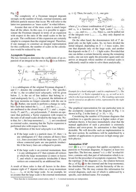
Fig. 2:<br />
Example for a hard subgraph γ and its complement Γ/γ. The<br />
integrand of γ is Taylor expanded in q2, q3, as well as in k,<br />
which is the loop momentum of Γ/γ. The resulting expression<br />
can be viewed as an effective vertex, represented by the right<br />
blob in Γ/γ.<br />
The graphical representation for one particular term in<br />
the asymptotic expansion of the diagram in FIg. 1 is<br />
shown in Fig. 2 in the limit q 2 1 ≫ M1 = M2.<br />
Considering the number of Feynman diagrams that<br />
contribute to a specific process at higher orders of perturbation<br />
theory, it becomes immediately clear that the<br />
manual application of such a procedure is extremely<br />
tedious and error-prone. Its automation is thus highly<br />
desirable. We will describe such an implementation in<br />
the next section. Its usefulness will be underlined by a<br />
number of applications to processes in high energy particle<br />
physics.<br />
Automation: EXP<br />
EXP [2] is a C++ program that applies asymptotic expansions<br />
to Feynman diagrams. It requires at least two<br />
input files. The first one, named “edia-file” in what follows,<br />
contains only that part of information which is relevant<br />
for the procedure of asymptotic expansion. This is<br />
the topology of the diagrams (i.e., the relation between<br />
the pi of Eq. (1) to the external and the loop momenta),<br />
the distribution of masses, and the hierarchy of the external<br />
scales. The file may contain this information for<br />
several diagrams, each one of which is addressed by a<br />
specific, user-defined name. For example,