2002 - Volume 1 - JEFF. Journal of Engineered Fibers and Fabrics
2002 - Volume 1 - JEFF. Journal of Engineered Fibers and Fabrics
2002 - Volume 1 - JEFF. Journal of Engineered Fibers and Fabrics

You also want an ePaper? Increase the reach of your titles
YUMPU automatically turns print PDFs into web optimized ePapers that Google loves.
A B<br />
C<br />
D<br />
Figure 1<br />
Simulated isotropic <strong>and</strong> anisotropic r<strong>and</strong>om samples<br />
(crimp k=1.35, density 20 fibers/mm2 ): (a) isotropic<br />
network; (b) anisotropic network; (c) polar plot <strong>of</strong> the<br />
isotropic fiber network; (d) polar plot <strong>of</strong> the<br />
anisotropic fiber network<br />
Simulation Results And Discussion<br />
A range <strong>of</strong> simulated nonwovens were generated with different<br />
conditions <strong>of</strong> anisotropy, fiber crimp, fiber clumping,<br />
<strong>and</strong> fiber spatial density. Figures 1 (a), (b), (c) <strong>and</strong> (d) show<br />
some simulated crimp fiber networks. Usually, in papermaking<br />
mean fiber length (i.e. L) ranges from 1.5–6 mm (Smook,<br />
1994). In our experiments we utilize short fibers, i.e. mean<br />
fiber length <strong>of</strong> 2 mm, <strong>and</strong> st<strong>and</strong>ard deviation <strong>of</strong> 0.5 mm. The<br />
density <strong>of</strong> the simulated samples in Figure 1 vary from 15 –<br />
70 fibers per mm 2 . The area represented in those images corresponds<br />
approximately to 100 mm 2 (i.e. approximately 10<br />
mm x 10 mm). Notice that Figures 1(a) <strong>and</strong> (b) show r<strong>and</strong>om<br />
isotropic <strong>and</strong> anisotropic simulated samples with 20 fibers per<br />
mm 2 , <strong>and</strong> k=1.35.<br />
Figures 1(c) <strong>and</strong> (d) show the polar plots obtained for those<br />
samples, using the technique proposed in (Scharcanski et. al.,<br />
1996), indicating that the sample shown in Figure 1(a) is in<br />
fact nearly isotropic (i.e. e=1.30), while the sample shown in<br />
Figure 1(b) is anisotropic (i.e. e=2.33).<br />
Both samples were simulated with the same density <strong>and</strong><br />
fiber length distributions. Nevertheless, we used s x =4 mm <strong>and</strong><br />
s y =4 mm to generate the nearly r<strong>and</strong>om sample. For image<br />
analysis purposes, the simulated images were sub-divided<br />
into approximately 200 x 200 square blocks, namely, pixels<br />
(i.e. each pixel is 25 x 10 –4 mm 2) , <strong>and</strong> after that, the density<br />
(i.e. pixels occupied by fibers) as well as void areas (i.e. pixels<br />
not occupied by fibers) were computed. Therefore, the<br />
A B<br />
C<br />
D<br />
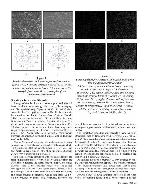
Figure 2<br />
Simulated isotropic samples with different fiber densities<br />
<strong>and</strong> degrees <strong>of</strong> flocculation<br />
(a) lower density r<strong>and</strong>om fiber network containing<br />
straight fibers only (crimp k=1.0, density 15<br />
fibers/mm2 ); (b) higher density flocculated network<br />
containing straight fibers only (crimp k=1.0, density<br />
30 fibers/mm2); (c) higher density r<strong>and</strong>om fiber network<br />
containing crimped fibers only (crimp k=1.3,<br />
density 30 fibers/mm2); (d) higher density flocculated<br />
fiber network containing crimped fibers only<br />
(crimp k=1.3, density 30 fibers/mm2)<br />
side <strong>of</strong> the square zones utilized for fiber density calculations<br />
correspond approximately to 50 microns (i.e. nearly one fiber<br />
width).<br />
Our simulation procedure can generate a wide range <strong>of</strong><br />
structures, such as those displayed in Figures 2(a), (b), (c)<br />
<strong>and</strong> (d). Two examples <strong>of</strong> isotropic fiber networks constituted<br />
by straight fibers (i.e. k = 1.0), with different fiber densities<br />
<strong>and</strong> degrees <strong>of</strong> flocculation (i.e. fiber clumping), are shown in<br />
Figures 2(a) <strong>and</strong> (b). Also, two examples <strong>of</strong> isotropic fiber<br />
networks constituted by crimped fibers (i.e. k = 1.3), with the<br />
same fiber densities, but different degrees <strong>of</strong> flocculation, are<br />
displayed in Figures 2(c) <strong>and</strong> (d).<br />
All statistics displayed in Figures 3–11 were obtained by simple<br />
image analysis techniques applied to the synthesized images<br />
<strong>of</strong> the simulated structures (e.g. detecting voids based on zones<br />
not occupied by fibers, or counting fiber crossings at zones/pixels<br />
as the pixel intensities generated by the simulation).<br />
Figures 3 <strong>and</strong> 4 show logarithmic scale plots <strong>of</strong> the mean<br />
versus the st<strong>and</strong>ard deviation <strong>of</strong> all voids occurring in each<br />
INJ Spring <strong>2002</strong> 25