- Page 1: RANDOM FIELDS AND THEIR GEOMETRY Ro
- Page 4 and 5: iv Contents 2.5 Orthogonal expansio
- Page 6 and 7: 1 Random fields 1.1 Random fields a
- Page 8 and 9: 1.2 Gaussian fields 3 • In applic
- Page 10 and 11: 1.2 Gaussian fields 5 A judicious c
- Page 12 and 13: 1.3 The Brownian family of processe
- Page 14 and 15: 1.3 The Brownian family of processe
- Page 16 and 17: 1.4 Stationarity 11 Then Aω and B
- Page 18 and 19: 1.4 Stationarity 13 operation +, if
- Page 20 and 21: 1.4 Stationarity 15 L 2 (P) ≡ L 2
- Page 22 and 23: 1.4 Stationarity 17 additional defi
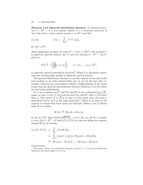
- Page 26 and 27: 1.4 Stationarity 21 and the terms i
- Page 28 and 29: W1 and W2, such that 26 (1.4.24) ft
- Page 30 and 31: moments, when they exist, are zero;
- Page 32 and 33: 1.4.5 Constant variance 1.4 Station
- Page 34 and 35: 1.4 Stationarity 29 ∆ where δij
- Page 36 and 37: Now use the spectral decomposition
- Page 38 and 39: 1.4 Stationarity 33 If T = R N unde
- Page 40 and 41: 1.5 Non-Gaussian fields 35 know the
- Page 42 and 43: 1.5 Non-Gaussian fields 37 In other
- Page 44 and 45: 2 Gaussian fields The aim of this C
- Page 46 and 47: 2.1 Boundedness and continuity 41 b
- Page 48 and 49: 2.1 Boundedness and continuity 43 T
- Page 50 and 51: should be taken as the definition o
- Page 52 and 53: 2.1 Boundedness and continuity 47 w
- Page 54 and 55: 2.2 Examples 2.2.1 Fields on R N 2.
- Page 56 and 57: 2.2 Examples 51 for |t| small enoug
- Page 58 and 59: To see why, endow the space R N ×
- Page 60 and 61: 2.2 Examples 55 The proof requires
- Page 62 and 63: canonical metric d, where (2.2.15)
- Page 64 and 65: 2.2 Examples 59 Similarly, again re
- Page 66 and 67: of a measure µ on RN , then by ana
- Page 68 and 69: 2.2 Examples 63 These inequalities
- Page 70 and 71: 2.2 Examples 65 Fix ε > 0 and supp
- Page 72 and 73: 2.3 Borell-TIS inequality 2.3 Borel
- Page 74 and 75:
2.3 Borell-TIS inequality 69 But th
- Page 76 and 77:
2.3 Borell-TIS inequality 71 the se
- Page 78 and 79:
2.3 Borell-TIS inequality 73 so tha
- Page 80 and 81:
2.4 Comparison inequalities 75 g, a
- Page 82 and 83:
2.5 Orthogonal expansions 77 which
- Page 84 and 85:
versa. Start with � S = u : T →
- Page 86 and 87:
2.5 Orthogonal expansions 81 With S
- Page 88 and 89:
2.5 Orthogonal expansions 83 where
- Page 90 and 91:
2.5 Orthogonal expansions 85 where
- Page 92 and 93:
2.6 Majorising measures 87 is alway
- Page 94 and 95:
2.6 Majorising measures 89 replacin
- Page 96 and 97:
2.6 Majorising measures 91 This Lem
- Page 98 and 99:
Finally, set Λ = min(Dµ, Dν). Th
- Page 100 and 101:
3 Geometry For this Chapter we are
- Page 102 and 103:
3.2 Basic integral geometry 97 fiel
- Page 104 and 105:
3.2 Basic integral geometry 99 Now
- Page 106 and 107:
and define (3.2.9) ϕ(A) = � h(A,
- Page 108 and 109:
3.3 Excursion sets again 103 drille
- Page 110 and 111:
espect to T at the level u. (3.3.4)
- Page 112 and 113:
3.3 Excursion sets again 107 this p
- Page 114 and 115:
3.3 Excursion sets again 109 will c
- Page 116 and 117:
3.3 Excursion sets again 111 FIGURE
- Page 118 and 119:
3.4 Intrinsic volumes 113 suitable
- Page 120 and 121:
3.4 Intrinsic volumes 115 Comparing
- Page 122 and 123:
functional ˜ ψu for which � �
- Page 124 and 125:
3.5 Manifolds and tensors 119 If a
- Page 126 and 127:
3.5 Manifolds and tensors 121 for a
- Page 128 and 129:
3.5 Manifolds and tensors 123 up th
- Page 130 and 131:
y (3.5.8) α ∧ β = (r + s)! A(α
- Page 132 and 133:
3.5 Manifolds and tensors 127 and t
- Page 134 and 135:
3.6 Riemannian manifolds 129 Simila
- Page 136 and 137:
3.6 Riemannian manifolds 131 The ba
- Page 138 and 139:
3.6 Riemannian manifolds 133 If θ
- Page 140 and 141:
3.6 Riemannian manifolds 135 Given
- Page 142 and 143:
3.6 Riemannian manifolds 137 manifo
- Page 144 and 145:
3.6 Riemannian manifolds 139 FIGURE
- Page 146 and 147:
3.6 Riemannian manifolds 141 and we
- Page 148 and 149:
3.6 Riemannian manifolds 143 With t
- Page 150 and 151:
3.6 Riemannian manifolds 145 We are
- Page 152 and 153:
3.7 Piecewise smooth manifolds 147
- Page 154 and 155:
3.7 Piecewise smooth manifolds 149
- Page 156 and 157:
3.7 Piecewise smooth manifolds 151
- Page 158 and 159:
3.7 Piecewise smooth manifolds 153
- Page 160 and 161:
and the homeomorphisms ψt are such
- Page 162 and 163:
3.8 Intrinsic volumes again 157 We
- Page 164 and 165:
3.8 Intrinsic volumes again 159 to
- Page 166 and 167:
3.9 Critical Point Theory 161 C 2 f
- Page 168 and 169:
� k 3.9 Critical Point Theory 163
- Page 170 and 171:
3.9 Critical Point Theory 165 What
- Page 172 and 173:
3.9 Critical Point Theory 167 [0, 1
- Page 174 and 175:
3.9 Critical Point Theory 169 and t
- Page 176 and 177:
4 Gaussian random geometry With the
- Page 178 and 179:
4.1 An expectation meta-theorem 173
- Page 180 and 181:
4.1 An expectation meta-theorem 175
- Page 182 and 183:
have 4.1 An expectation meta-theore
- Page 184 and 185:
4.1 An expectation meta-theorem 179
- Page 186 and 187:
4.1 An expectation meta-theorem 181
- Page 188 and 189:
4.1 An expectation meta-theorem 183
- Page 190 and 191:
4.1 An expectation meta-theorem 185
- Page 192 and 193:
4.2 Suitable regularity and Morse f
- Page 194 and 195:
our manifold as usual as (4.2.2) 4.
- Page 196 and 197:
4.4 Higher moments 191 Take α(t) =
- Page 198 and 199:
4.5 Preliminary Gaussian computatio
- Page 200 and 201:
implying 4.5 Preliminary Gaussian c
- Page 202 and 203:
4.6 Mean Euler characteristics: Euc
- Page 204 and 205:
4.6 Mean Euler characteristics: Euc
- Page 206 and 207:
all out again. We start with 4.6 Me
- Page 208 and 209:
4.6 Mean Euler characteristics: Euc
- Page 210 and 211:
4.6 Mean Euler characteristics: Euc
- Page 212 and 213:
4.6 Mean Euler characteristics: Euc
- Page 214 and 215:
4.7 The meta-theorem on manifolds 2
- Page 216 and 217:
4.7 The meta-theorem on manifolds 2
- Page 218 and 219:
4.8 Riemannian structure induced by
- Page 220 and 221:
4.8 Riemannian structure induced by
- Page 222 and 223:
4.8 Riemannian structure induced by
- Page 224 and 225:
4.8 Riemannian structure induced by
- Page 226 and 227:
4.9 Another Gaussian computation 22
- Page 228 and 229:
4.10.1 Manifolds without boundary 4
- Page 230 and 231:
4.10 Mean Euler characteristics: Ma
- Page 232 and 233:
4.10 Mean Euler characteristics: Ma
- Page 234 and 235:
4.10 Mean Euler characteristics: Ma
- Page 236 and 237:
4.11 Examples 231 Stationary fields
- Page 238 and 239:
4.11 Examples 233 its own curvature
- Page 240 and 241:
4.12 Chern-Gauss-Bonnet Theorem 4.1
- Page 242 and 243:
References [1] R. J. Adler. The Geo
- Page 244 and 245:
References 283 [25] R. M. Dudley. L
- Page 246 and 247:
References 285 [58] John M. Lee. In
- Page 248 and 249:
References 287 [88] D. Slepian. On