Lecture 5: Polarization and Related Antenna Parameters

Lecture 5: Polarization and Related Antenna Parameters
(Polarization of EM fields – revision. Polarization vector. Antenna
polarization. Polarization loss factor and polarization efficiency.)
1. Polarization of EM fields
The polarization of the EM field describes the orientation of its vectors at a
given point and how it varies with time. In other words, it describes the way the
direction and magnitude of the field vectors (usually E) change in time.
Polarization is associated with TEM time-harmonic waves where the H vector
relates to the E vector simply by H rˆ E
/ .
In antenna theory, we are concerned with the polarization of the field in the
plane orthogonal to the direction of propagation—this is the plane defined by
the vectors of the far field. Remember that the far field is a quasi-TEM field.
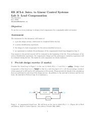
The polarization is the locus traced by the extremity of the time-varying field
vector at a fixed observation point.
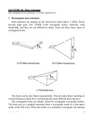
According to the shape of the trace, three types of polarization exist for
harmonic fields: linear, circular and elliptical. Any polarization can be
represented by two orthogonal linear polarizations, ( Ex, E y)
or ( EH, E V),
whose
fields are out of phase by an angle of L .
z
y
E
x
y
z
E
x
z E
(a) linear polarization (b) circular polarization (c) elliptical polarization
Nikolova 2012 1
y
x

If L 0 or n , then linear polarization results.
t
0
t e ( t)
only
H
e ( t)
only
H
t
e () t
e () t
Animation: Linear Polarization, L 0,
Ex Ey
Nikolova 2012 2
0
t H
e () t
V
V
e () t
H

If / 2 (90 ) and | E | | E | , then circular polarization results.
t1
L
x y
t t
2 1 /2
Animation: Clockwise Circular Rotation
In the most general case, elliptical polarization is defined.
t
0
t /2
Animation: Counter-clockwise Elliptical Rotation
It is also true that any type of polarization can be represented by a righthand
circular and a left-hand circular polarizations ( E L,
E R ). Next, we review
the above statements and definitions, and introduce the new concept of
polarization vector.
Nikolova 2012 3

2. Field polarization in terms of two orthogonal linearly polarized
components
The polarization of any field can be represented by a set of two orthogonal
linearly polarized fields. Assume that locally a far-field wave propagates along
the z-axis. The far-zone field vectors have only transverse components. Then,
the set of two orthogonal linearly polarized fields along the x-axis and along
the y-axis, is sufficient to represent any TEMz field. We use this arrangement to
introduce the concept of polarization vector.
The field (time-dependent or phasor vector) is decomposed into two
orthogonal components:
e ex ey E Ex E y,
(5.1)
ex Excos tzxˆ e E cos t z
yˆ
Ex Exxˆ
E EejLyˆ.
(5.2)
y y L
y y
At a fixed position (assume z 0),
equation (5.1) can be written as
e( t) xˆEcostyˆEcos( t )
x y L
ˆ E ˆ E e j L
E x y
x y
Case 1: Linear polarization: Ln, n
0,1,2,
e( t) xˆEcos( t) yˆEcos(
t n
)
E y
y
(a)
x y
E xˆE yˆE
2k
L
0 E
E x
x
x y
Ey arctan
E
x
(2k1)
(5.3)
(5.4)
Nikolova 2012 4
E
y
L
E
(b)
y
0
Ex
x

Case 2: Circular polarization:
3
t
5
2
t
4
t 3
t
4
Ex Ey Em and L n, n 0,1,2,
2
e( t) xˆEcos( t) yˆEcos[
t ( / 2 n
)]
x y
E E ( xˆ jyˆ)
E E ( xˆ jyˆ)
m
L2n 2
y
z
t
2
m
7
t
4
t
4
t 0
x
If z ˆ is the direction of
propagation: counterclockwise
(CCW) or left-hand polarization
t
t 5
t
4
E E ( xˆ jyˆ)
t y
2
L2n 2
3
4
3
t
2
(5.5)
t
4
t 0
x
7
t
4
Note that the sense of rotation changes if the direction of propagation changes.
In the example above, if the wave propagates along z, ˆ the plot to the left,
where E Em( xˆ jy
ˆ)
, corresponds to a right-hand wave, while the plot to the
right, where E E ( xˆ jy
ˆ)
, corresponds to a left-hand wave.
m
If ˆ
z is the direction of
propagation: clockwise (CW) or
right-hand polarization
Nikolova 2012 5
m
z

A snapshot of the field vector (at a particular moment of time) along the axis
of propagation is given below for a left-hand circularly polarized wave
travelling along z.
Pick an observing position along the z axis and
imagine that the whole helical trajectory of the tip of the field vector moves
along z.
Are you going to see the vector rotating clockwise or counterclockwise
(as you look toward z ). (Ans.: counter-clockwise)
y
Case 3: Elliptic polarization
x
The field vector at a given point traces an ellipse as a function of time. This
is the most general type of polarization, obtained for any phase difference
and any ratio ( Ex / E y)
. Mathematically, the linear and the circular
polarizations are special cases of the elliptical polarization. In practice,
however, the term elliptical polarization is used to indicate polarizations other
than linear or circular.
( t) ˆExcostˆEycos( t L)
ˆEˆEejL
e x y
(5.6)
E x y
x y
z
Nikolova 2012 6

Show that the trace of the time-dependent vector is an ellipse:
e ( t) E (cost cos sin t sin )
y y L L
ex() t
ex() t
cost
and sint 1
E
x
E
x
2
ex( t) ex( t)
ey t ey t
L L
E
x E
x Ey Ey
sin2
2
( )
cos
( )
or (dividing both sides by sin2 L ),
1 x2( t) 2 x( t) y( t)cos 2
L y ( t)
,
where
ex( t) cost
xt () ,
Ex
sinLsinL ey() t cos( tL) yt () .
E sin sin
(5.7)
y L L
Equation (5.7) is the equation of an ellipse centered in the xy plane. It
describes the trajectory of a point of coordinates x(t) and y(t), i.e., normalized
ex() t and ey() t values, along an ellipse where the point moves with an angular
frequency .
As the circular polarization, the elliptical polarization can be right-handed
or left-handed, depending on the relation between the direction of propagation
and the direction of rotation.
e () t
y
major axis (2 OA)
E
Ey
minor axis (2 OB)
Nikolova 2012 7
2
Ex
ex() t
2

The parameters of the polarization ellipse are given below. Their derivation
is given in Appendix I.
a) major axis (2 OA)
OA =
1
E22 x Ey
2
E4 4 2 2 2
x Ey Ex Ey cos(2 L
)
(5.8)
b) minor axis (2 OB)
OB =
1
E22 x Ey
2
E4 4 2 2 2
x Ey Ex Ey cos(2 L
)
(5.9)
c) tilt angle
1 2EE
x y
arctan cos
2
2 2
L
Ex Ey
(5.10)
Note: Eq. (5.10) produces an infinite number of angles, τ = (arctanA)/2
n /2,
n = 1,2,….Thus, it gives not only the angle which the major
axis of the ellipse forms with the x axis but also the angle of the minor
axis with the x axis. In spherical coordinates, τ is usually specified
with respect to the ˆ θ direction
d) axial ratio
Nikolova 2012 8
A
major axis OA
AR (5.11)
minor axis OB
Note: The linear and circular polarizations as special cases of the elliptical
polarization:
If L 2n
2 and Ex Ey,
then OA OB Ex Ey;
the ellipse
becomes a circle.
If L n,
then OB 0 and arctan( Ey / Ex)
; the ellipse collapses
into a line.

3. Field polarization in terms of two circularly polarized components
The representation of a complex vector field in terms of circularly polarized
components is somewhat less easy to perceive but it is actually more useful in
the calculation of the polarization ellipse parameters. This time, the total field
phasor is represented as the superposition of two circularly polarized waves,
one right-handed and the other left-handed. For the case of a wave propagating
along z [see Case 2 and Eq. (5.5)],
E E ( xˆ jyˆ ) E ( xˆ jy
ˆ)
. (5.12)
R L
Here, ER and EL are in general complex phasors. Assuming a relative phase
difference of C L R,
one can write (5.12) as
e ( ˆ ˆ) j C
R j eLe( ˆ jˆ
)
E x y x y , (5.13)
where e R and e L are real numbers.
The relations between the linear-component and the circular-component
representations of the field polarization are easily found as
E xˆ( E E ) y ˆ j( E E )
(5.14)
R L R L
E E
x y
Ex ER EL
E j( E E)
y R L
ER 0.5( Ex jEy
)
E 0.5( E jE )
L x y
4. Polarization vector and polarization ratio
The polarization vector is the normalized phasor of the electric field vector.
It is a complex-valued vector of unit magnitude, i.e., ρˆ ρ ˆ 1.
L L
x y j L
2 2
L e Em Ex Ey
Em Em Em
(5.15)
(5.16)
E E E
ρˆ xˆ y ˆ ,
(5.17)
The polarization vector takes the following specific forms:
Case 1: Linear polarization
Nikolova 2012 9

Ex
Ey
ρˆ xˆ y ˆ ,
Em Em
Em E2 2
x Ey
(5.18)
where E x and E y are real numbers.
Case 2: Circular polarization
ρˆ L
1
xˆ jy ˆ ,
2
Em 2Ex 2Ey
(5.19)
The polarization ratio is the ratio of the phasors of the two orthogonal
polarization components. In general, it is a complex number:
E j L
y Eye EV
r L
L rLe or rL
(5.20)
E E E
x x H
Point of interest: In the case of circular-component representation, the
polarization ratio is defined as
r r e
j
C
C . (5.21)
EL
C R
The circular polarization ratio r C is of particular interest since the axial ratio of
the polarization ellipse AR can be expressed as
rC
1
AR . (5.22)
r 1
Besides, its tilt angle with respect to the y (vertical) axis is simply
/2
Nikolova 2012 10
C
E
V C . (5.23)
Comparing (5.10) and (5.23) readily shows the relation between the phase
difference δC of the circular-component representation and the linear
polarization ratio r j L
L rLe :
2rL
C arctan cos
1 2
L
r
.
(5.24)
L
We can calculate r C from the linear polarization ratio r L making use of (5.11)
and (5.22):

C 1
1 r2 L 1 r4 2 2
L rL
cos(2 L
)
C 1 1 2
L 1 4 2 2
L L cos(2 L
)
r
AR
. (5.25)
r r r r
Using (5.24) and (5.25) allows switching between the representation of the
wave polarization in terms of linear and circular components.
5. Antenna polarization
The polarization of a transmitting antenna is the polarization of its
radiated wave in the far zone. The polarization of a receiving antenna is the
polarization of a plane wave, incident from a given direction, which, for a
given power flux density, results in maximum available power at the antenna
terminals.
The antenna polarization is defined by the polarization vector of the
radiated (transmitted) wave. Notice that the polarization vector of a wave in the
coordinate system of the transmitting antenna is represented by its complex
conjugate in the coordinate system of the receiving antenna:
ˆr ( ˆt
w w) ρ ρ . (5.26)
The conjugation is without importance for a linearly polarized wave since its
polarization vector is real. It is, however, important in the cases of circularly
and elliptically polarized waves.
This is illustrated in the figure below with a right-hand CP wave. Let the
t t t
coordinate triplet ( x1, x2, x 3)
represents the coordinate system of the
r r r
transmitting antenna while ( x1, x2, x 3 ) represents that of the receiving antenna.
Note that in antenna theory the plane of polarization is usually given in
spherical coordinates by ( xˆ ˆ
1, xˆ2) ( θφ , ˆ ) and the third axis obeys xˆ 1 xˆ2x ˆ 3,
i.e., xˆ3r. ˆ Since the transmitting and receiving antennas face each other, their
t r
coordinate systems are oriented so that xˆ3 x
ˆ3
(i.e., ˆr ˆt
r r
). If we align the
axes ˆ1 t x and ˆ1 r x , then ˆt 2 ˆr
x x
2 must hold. This changes the sign in the
imaginary part of the wave polarization vector.
Nikolova 2012 11

RHCP wave
t
x2
t
x1
ˆ ˆ t
k x
t /2
x
t 1 t t
ρˆ w ( xˆ1 jxˆ2)
2
3
t
3
Nikolova 2012 12
r
x3
r
x1
t 0
t 0
r
x2
ˆ ˆ 3
r
k x
t /2
r 1 r r
ρˆ w ( xˆ1 jxˆ2)
2
Bearing in mind the definitions of antenna polarization in transmitting and
receiving modes, we conclude that the transmitting-mode polarization vector
of an antenna is the conjugate of its receiving-mode polarization vector.
6. Polarization loss factor and polarization efficiency
Generally, the polarization of the receiving antenna is not the same as the
polarization of the incident wave. This is called polarization mismatch.
The polarization loss factor (PLF) characterizes the loss of EM power
because of polarization mismatch:
PLF | ρˆ ˆ | 2
iρ a . (5.27)
The above definition is based on the representation of the incident field and the
antenna polarization by their polarization vectors. If the incident field is
Ei Ei
mρ ˆ i,
then the field of the same magnitude that would produce maximum received
power at the antenna terminals is
E Ei
ρ ˆ .
a m a

If the antenna is polarization matched, then PLF 1,
and there is no
polarization power loss. If PLF 0,
then the antenna is incapable of receiving
the signal.
0 PLF 1
(5.28)
The polarization efficiency means the same as the PLF.
Examples
Example 5.1. The electric field of a linearly polarized EM wave is
i ˆ E ( , ) j z
m x y e
E x
.
It is incident upon a linearly polarized antenna whose polarization is
Ea ( xˆ y ˆ)
Er ( , , ) .
Find the PLF.
Nikolova 2012 13

PLF xˆ
1
( xˆ y ˆ)
2
1
2
PLF 10log 0.5 3 dB
[dB] 10
2
Example 5.2. A transmitting antenna produces a far-zone field, which is
RH circularly polarized. This field impinges upon a receiving antenna,
whose polarization (in transmitting mode) is also RH circular. Determine
the PLF.
Both antennas (the transmitting one and the receiving one) are RH
circularly polarized in transmitting mode. Assume that a transmitting
antenna is located at the center of a spherical coordinate system. The farzone
field it would produce is described as
E far E ˆ
m cost ˆ cos( t
/ 2)
θ φ
It is a RH circularly polarized field with respect to the outward radial
direction. Its polarization vector is
θˆjφˆ ρ ˆ .
2
This is exactly the polarization vector of the transmitting antenna.
x
z
E
r
Nikolova 2012 14
E
y

This same field Ε far is incident upon a receiving antenna, which has the
polarization vector ρˆ ( ˆ
a θa jφ
ˆa)
/ 2 in its own coordinate system
( ra , a, a)
. However, Ε far propagates along r ˆa in the ( ra , a, a)
coordinate system, and, therefore, its polarization vector becomes
θˆ a jφˆa
ρ ˆ i .
2
The PLF is calculated as
ˆ ˆ ˆ ˆ 2
2 | ( θa jφa)( θa jφa)
|
PLF | ρˆiρ ˆa
| 1,
PLF[dB] 10log101 0.
4
There are no polarization losses.
Exercise: Show that an antenna of RH circular polarization (in transmitting
mode) cannot receive LH circularly polarized incident wave (or a wave
emitted by a left-circularly polarized antenna).
Appendix I
Find the tilt angle , the length of the major axis OA, and the length of the
minor axis OB of the ellipse described by the equation:
2
x x
( ) ( )
2 e ( t) e ( t)
ey t ey t
sin 2 cos
E
x E
x Ey Ey
ey() t
major axis (2 OA)
E
Ey
minor axis (2 OB)
ex() t
Nikolova 2012 15
Ex
2
.
(A-1)

Equation (A-1) can be written as
a x2bxycy2 1,
(A-2)
where
x ex() t and y ey() t are the coordinates of a point of the ellipse
centered in the xy plane;
1
a ;
E2sin2 x
2cos
b ;
EE sin2
x y
1
c .
E2sin2 y
After dividing both sides of (A-2) by ( xy ) , one obtains
x y 1
a b c .
(A-3)
y x xy
y ey() t
Introducing , one obtains that
x ex() t
2 1
x
c2b a
1
( ) (1 ) .
2
2 x2 y2 x2
2
c2b a
Here, is the distance from the center of the coordinate system to the point on
the ellipse. We want to know at what values of the maximum and the
minimum of occur ( min , max ). This will produce the tilt angle . We also
want to know the values of max (major axis) and min (minor axis). Then, we
have to solve
d(
2)
0,
or
d
2 2( ac) m m
1 0,
where m min, max
. (A-5)
b
(A-5) is solved for the angle τ, which relates to ξmax as
tan y/ x
.
(A-6)
max max
(A-4)
Nikolova 2012 16

Substituting (A-6) in (A-5) yields:
sin sin
2C 1 0
cos cos
where
2 2
ac Ey Ex
C .
b 2ExEycos Multiplying both sides of (A-7) by cos2 and re-arranging results in
2 2 cos sin 2C sin cos 0.
Thus, the solution of (A-7) is
or
2
cos(2 ) Csin(2
)
tan(2 ) 1/ C
1 2EE cos
arctan ;
x y
1 2 2 2 1 .
2 Ex Ey
2
The angles τ1 and τ2 are the angles between the major and minor axes with the x
axis. Substituting 1 and 2 back in (see A-4) yields the expressions for OA
and OB.
(A-7)
(A-8)
Nikolova 2012 17