
You also want an ePaper? Increase the reach of your titles
YUMPU automatically turns print PDFs into web optimized ePapers that Google loves.
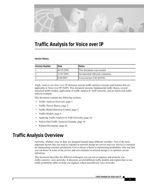
<strong>Traffic</strong> <strong>Analysis</strong> <strong>for</strong> <strong>Voice</strong> <strong>over</strong> <strong>IP</strong><br />
Version History<br />
Version Number Date Notes<br />
1 06/25/2001 This document was created.<br />
2 11/01/2001 Incorporated editorial comments.<br />
3 6/20/2007 Corrected per CSCsj34541.<br />
<strong>Traffic</strong> <strong>Analysis</strong> <strong>for</strong> <strong>Voice</strong> <strong>over</strong> <strong>IP</strong> discusses various traffic analysis concepts and features that are<br />
applicable to <strong>Voice</strong> <strong>over</strong> <strong>IP</strong> (Vo<strong>IP</strong>). This document presents fundamental traffic theory, several<br />
statistical traffic models, application of traffic analysis to Vo<strong>IP</strong> networks, and an end-to-end traffic<br />
analysis example.<br />
This document contains the following sections:<br />
• <strong>Traffic</strong> <strong>Analysis</strong> Overview, page 1<br />
• <strong>Traffic</strong> Theory Basics, page 2<br />
• <strong>Traffic</strong> Model Selection Criteria, page 5<br />
• <strong>Traffic</strong> Models, page 8<br />
• Applying <strong>Traffic</strong> <strong>Analysis</strong> to Vo<strong>IP</strong> Networks, page 14<br />
• End-to-End <strong>Traffic</strong> <strong>Analysis</strong> Example, page 18<br />
• Related Documents, page 20<br />
<strong>Traffic</strong> <strong>Analysis</strong> Overview<br />
Networks, whether voice or data, are designed around many different variables. Two of the most<br />
important factors that you need to consider in network design are service and cost. Service is essential<br />
<strong>for</strong> maintaining customer satisfaction. Cost is always a factor in maintaining profitability. One way that<br />
you can factor in some of the service and cost elements in network design is to optimize circuit<br />
utilization.<br />
This document describes the different techniques you can use to engineer and properly size<br />
traffic-sensitive voice networks. It discusses several different traffic models and explain how to use<br />
traffic probability tables to help you engineer robust and efficient voice networks.<br />
<strong>Traffic</strong> <strong>Analysis</strong> <strong>for</strong> <strong>Voice</strong> <strong>over</strong> <strong>IP</strong><br />
1
<strong>Traffic</strong> Theory Basics<br />
<strong>Traffic</strong> Theory Basics<br />
2<br />
<strong>Traffic</strong> <strong>Analysis</strong> <strong>for</strong> <strong>Voice</strong> <strong>over</strong> <strong>IP</strong><br />
<strong>Traffic</strong> <strong>Analysis</strong> <strong>for</strong> <strong>Voice</strong> <strong>over</strong> <strong>IP</strong><br />
Network designers need a way to properly size network capacity, especially as networks grow. <strong>Traffic</strong><br />
theory enables network designers to make assumptions about their networks based on past experience.<br />
<strong>Traffic</strong> is defined as either the amount of data or the number of messages <strong>over</strong> a circuit during a given<br />
period of time. <strong>Traffic</strong> also includes the relationship between call attempts on traffic-sensitive<br />
equipment and the speed with which the calls are completed. <strong>Traffic</strong> analysis enables you to determine<br />
the amount of bandwidth you need in your circuits <strong>for</strong> data and <strong>for</strong> voice calls. <strong>Traffic</strong> engineering<br />
addresses service issues by enabling you to define a grade of service or blocking factor. A properly<br />
engineered network has low blocking and high circuit utilization, which means that service is increased<br />
and your costs are reduced.<br />
There are many different factors that you need to take into account when analyzing traffic. The most<br />
important factors are described in the following sections:<br />
• <strong>Traffic</strong> Load Measurement<br />
• Grade of Service<br />
• <strong>Traffic</strong> Types<br />
<strong>Traffic</strong> Load Measurement<br />
• Sampling Methods<br />
Of course, other factors might affect the results of traffic analysis calculations, but these are the main<br />
ones. You can make assumptions about the other factors.<br />
In traffic theory, you measure traffic load. <strong>Traffic</strong> load is the ratio of call arrivals in a specified period<br />
of time to the average amount of time taken to service each call during that period. These measurement<br />
units are based on Average Hold Time (AHT). AHT is the total time of all calls in a specified period<br />
divided by the number of calls in that period, as shown in the following example:<br />
(3976 total call seconds)/(23 calls) = 172.87 sec per call = AHT of 172.87 seconds<br />
The two main measurement units used today to measure traffic load are erlangs and centum call seconds<br />
(CCS).<br />
One erlang is 3600 seconds of calls on the same circuit, or enough traffic load to keep one circuit busy<br />
<strong>for</strong> 1 hour. <strong>Traffic</strong> in erlangs is the product of the number of calls times AHT divided by 3600, as shown<br />
in the following example:<br />
(23 calls * 172.87 AHT)/3600 = 1.104 erlangs<br />
One CCS is 100 seconds of calls on the same circuit. <strong>Voice</strong> switches generally measure the amount of<br />
traffic in CCS.<br />
<strong>Traffic</strong> in CCS is the product of the number of calls times the AHT divided by 100, as shown in the<br />
following example:<br />
(23 calls * 172.87 AHT)/100 = 39.76 CCS<br />
Which unit you use depends highly on the equipment you use and what unit of measurement they record<br />
in. Many switches use CCS because it is easier to work with increments of 100 rather than 3600. Both<br />
units are recognized standards in the field. The following is how the two relate: 1 erlang = 36 CCS.<br />
Although you can take the total call seconds in an hour and divide that amount by 3600 seconds to<br />
determine the traffic in erlangs, you can also use averages of various time periods. These averages allow<br />
you to use more sample periods and determine the proper traffic.
<strong>Traffic</strong> <strong>Analysis</strong> <strong>for</strong> <strong>Voice</strong> <strong>over</strong> <strong>IP</strong><br />
Busy Hour <strong>Traffic</strong><br />
Network Capacity Measurements<br />
Grade of Service<br />
<strong>Traffic</strong> Types<br />
<strong>Traffic</strong> <strong>Analysis</strong> <strong>for</strong> <strong>Voice</strong> <strong>over</strong> <strong>IP</strong><br />
<strong>Traffic</strong> Theory Basics<br />
You commonly measure network traffic load during the busiest hour because this period represents the<br />
maximum traffic load that your network must support. The result gives you a traffic load measurement<br />
commonly referred to as the Busy Hour <strong>Traffic</strong> (BHT). There are times when you cannot do a thorough<br />
sampling or you have only an estimate of how many calls you are handling daily. In such a<br />
circumstance, you can usually make assumptions about your environment, such as average number of<br />
calls per day and the AHT. In the standard business environment, the busy hour of any given day<br />
accounts <strong>for</strong> approximately 15 to 20 percent of the traffic <strong>for</strong> that day. In your computations, you<br />
generally use 17 percent of the total daily traffic to represent the peak hour traffic. In many business<br />
environments, an acceptable AHT is generally assumed to be 180 to 210 seconds. You can use these<br />
estimates if you ever need to determine trunking requirements without having more complete data.<br />
Among the many ways to measure network capacity are the following:<br />
• Busy Hour Call Attempts (BHCA)<br />
• Busy Hour Call Completions (BHCC)<br />
• Calls per Second (CPS)<br />
All of these measurements are based on the number of calls. Although these measurements do describe<br />
network capacity, they are fairly meaningless to traffic analysis because they do not consider the hold<br />
time of the call. You need to use these measurements in conjunction with an AHT to derive a BHT that<br />
you can use <strong>for</strong> traffic analysis.<br />
Grade of Service (GoS) is defined as the probability that calls will be blocked while attempting to seize<br />
circuits. It is written as P.xx blocking factor or blockage, where xx is the percentage of calls that are<br />
blocked <strong>for</strong> a traffic system. For example, traffic facilities requiring P.01 GoS define a 1 percent<br />
probability of callers being blocked to the facilities. A GoS of P.00 is rarely requested and will rarely<br />
happen because to be 100 percent sure that there is no blocking, you would have to design a network<br />
where the caller to circuit ratio is 1:1. Also, most traffic <strong>for</strong>mulas assume that there are an infinite<br />
number of callers.<br />
You can use the telecommunications equipment that is offering the traffic to record the data described.<br />
Un<strong>for</strong>tunately, most of the samples received are based on the carried traffic on the system and not the<br />
offered traffic load.<br />
Carried traffic is the traffic that is actually serviced by telecommunications equipment. Offered traffic<br />
is the actual amount of traffic attempts on a system. Note that the difference in the two can cause some<br />
inaccuracies in your calculation.<br />
The greater the amount of blockage you have, the greater the difference between carried and offered<br />
load. You can use the following <strong>for</strong>mula to calculate offered load from carried load:<br />
Offered load = carried load/(1 – blocking factor)<br />
3
<strong>Traffic</strong> Theory Basics<br />
Sampling Methods<br />
4<br />
<strong>Traffic</strong> <strong>Analysis</strong> <strong>for</strong> <strong>Voice</strong> <strong>over</strong> <strong>IP</strong><br />
<strong>Traffic</strong> <strong>Analysis</strong> <strong>for</strong> <strong>Voice</strong> <strong>over</strong> <strong>IP</strong><br />
Un<strong>for</strong>tunately, this <strong>for</strong>mula does not take into account any retries that might happen when a caller is<br />
blocked. You can use the following <strong>for</strong>mula to take the retry rate into account:<br />
Offered load = carried load * Offered Load Adjustment Factors (OAF)<br />
OAF = [1.0 – (R * blocking factor)]/(1.0 – blocking factor)<br />
Where R is a percentage of retry probability. For example, R = 0.6 <strong>for</strong> a 60 percent retry rate.)<br />
The accuracy of your traffic analysis will also depend on the accuracy of your sampling methods. The<br />
following parameters will change the represented traffic load:<br />
• Weekdays versus weekends<br />
• Holidays<br />
• Type of traffic (modem versus traditional voice)<br />
• Apparent versus offered load<br />
• Sample period<br />
• Total number of samples taken<br />
• Stability of the sample period<br />
Probability theory states that to accurately assess voice network traffic, you need to have at least 30 of<br />
the busiest hours of a voice network in the sampling period. Although this is a good starting point, other<br />
variables can skew the accuracy of this sample. You cannot take the top 30 out of 32 samples and expect<br />
that sampling to be an accurate picture of the network. To get the most accurate results, you need to take<br />
as many samples of the offered load as possible. Alternatively, if you take samples throughout the year,<br />
your results can be skewed as your year-to-year traffic load increases or decreases. The International<br />
Telecommunication Union Telecommunication Standardization Sector (ITU-T) makes<br />
recommendations on how you can accurately sample a network to dimension it properly.<br />
The ITU-T recommends that public switched telephone network (PSTN) connections measurement or<br />
read-out periods be 60 minutes and/or 15-minute intervals. These intervals are important because they<br />
let you summarize the traffic intensity <strong>over</strong> a period of time. If you take measurements throughout the<br />
day, you can find the peak hour of traffic in any given day. There are two recommended ways to<br />
determine the peak daily traffic, as follows:<br />
• Daily Peak Period (DPP) records the highest traffic volume measured during a day. This method<br />
requires continuous measurement and is typically used in environments where the peak hour may<br />
be different from day to day.<br />
• Fixed Daily Measurement Interval (FDMI) requires measurements only during the predetermined<br />
peak periods. It is used when traffic patterns are somewhat predictable and peak periods occur at<br />
regular intervals. Business traffic usually peaks around 10:00 a.m. to 11:00 a.m. and 2:00 p.m. to<br />
3:00 p.m.<br />
In the example in Table 1, using FDMI sampling, you see that the hour with the highest total traffic load<br />
is 10 a.m., with a total traffic load of 60.6 erlangs.<br />
Table 1 Daily Peak Period Measurement<br />
Hour Monday Tuesday Wednesday Thursday Friday Total Load<br />
9:00 a.m. 12.7 11.5 10.8 11.0 8.6 54.6<br />
10:00 a.m. 12.6 11.8 12.5 12.2 11.5 60.6
<strong>Traffic</strong> <strong>Analysis</strong> <strong>for</strong> <strong>Voice</strong> <strong>over</strong> <strong>IP</strong><br />
The example in Table 2 uses DPP to calculate total traffic load.<br />
<strong>Traffic</strong> Model Selection Criteria<br />
You also need to divide the daily measurements into groups that have the same statistical behavior. The<br />
ITU-T defines these groups as: workdays, weekend days, and yearly exceptional days. Grouping<br />
measurements that have the same statistical behavior becomes important because exceptionally high<br />
call volume days (such as Christmas Day and Mother’s Day) might skew the results.<br />
ITU-T Recommendation E.492 includes recommendations <strong>for</strong> determining the normal and high load<br />
traffic intensities <strong>for</strong> the month. Per ITU-T recommendation E.492, the normal load traffic intensity <strong>for</strong><br />
the month is defined as the fourth highest daily peak traffic. If you select the second highest<br />
measurement <strong>for</strong> the month, it will result in the high load traffic intensity <strong>for</strong> the month. The result<br />
allows you to define expected monthly traffic load.<br />
<strong>Traffic</strong> Model Selection Criteria<br />
Now that you know what measurements are needed, you can determine how to use them. You need to<br />
pick the appropriate traffic model. The key elements to picking the appropriate model are described in<br />
the following sections:<br />
• Call Arrival Patterns<br />
• Blocked Calls<br />
• Number of Sources<br />
• Holding Times<br />
Call Arrival Patterns<br />
Table 1 Daily Peak Period Measurement (continued)<br />
Hour Monday Tuesday Wednesday Thursday Friday Total Load<br />
11:00 a.m. 11.1 11.3 11.6 12.0 12.3 58.3<br />
12:00 p.m. 9.2 8.4 8.9 9.3 9.4 45.2<br />
1:00 p.m. 10.1 10.3 10.2 10.6 9.8 51.0<br />
2:00 p.m. 12.4 12.2 11.7 11.9 11.0 59.2<br />
3:00 p.m. 9.8 11.2 12.6 10.5 11.6 55.7<br />
4:00 p.m. 10.1 11.1 10.8 10.5 10.2 52.7<br />
Table 2 Using DDP to Calculate Total <strong>Traffic</strong> Load<br />
Monday Tuesday Wednesday Thursday Friday Total Load<br />
Peak <strong>Traffic</strong> 12.7 12.2 12.5 12.2 12.3 61.9<br />
Peak Time 9:00 a.m. 2:00 p.m. 10:00 a.m. 10:00 a.m. 11:00 a.m.<br />
The first step in choosing the proper traffic model is to determine the call arrival pattern. Call arrival<br />
patterns are important in choosing a traffic model because different arrival patterns affect traffic<br />
facilities differently.<br />
The three main call arrival patterns are as follows and are described in the following sections:<br />
<strong>Traffic</strong> <strong>Analysis</strong> <strong>for</strong> <strong>Voice</strong> <strong>over</strong> <strong>IP</strong><br />
5
<strong>Traffic</strong> Model Selection Criteria<br />
Smooth Call Arrival Pattern<br />
Peaked Call Arrival Pattern<br />
6<br />
• Smooth Call Arrival Pattern<br />
• Peaked Call Arrival Pattern<br />
• Random Call Arrival Pattern<br />
<strong>Traffic</strong> <strong>Analysis</strong> <strong>for</strong> <strong>Voice</strong> <strong>over</strong> <strong>IP</strong><br />
<strong>Traffic</strong> <strong>Analysis</strong> <strong>for</strong> <strong>Voice</strong> <strong>over</strong> <strong>IP</strong><br />
A smooth or hypo-exponential traffic pattern occurs when there is not a great amount of variation in<br />
traffic. Call hold time and call interarrival times are predictable, allowing you to predict traffic in any<br />
given instance when there are a finite number of sources. For example, suppose you were designing a<br />
voice network <strong>for</strong> an outbound telemarketing company, where a few agents spend all day on the phone.<br />
Suppose that in a one-hour period, you could expect 30 sequential calls of 2 minutes each. You would<br />
then need to allocate one trunk to handle the calls <strong>for</strong> the hour.<br />
For a smooth call arrival pattern, a graph of calls versus time might look like Figure 1.<br />
Figure 1 Smooth Call Arrival Pattern<br />
Calls<br />
Time<br />
A peaked traffic pattern has big spikes in traffic from the mean. This call arrival pattern is also known<br />
as a hyperexponential arrival pattern. Peaked traffic patterns demonstrate why it might not be a good<br />
idea to include Mother's Day and Christmas Day in a traffic study. There might be times when you<br />
would want to engineer roll<strong>over</strong> trunk groups to handle this kind of traffic pattern. In general, however,<br />
to handle this kind of traffic pattern you would need to allocate enough resources to handle the peak<br />
traffic. For example, to handle 30 calls all at once, you would need 30 trunks.<br />
A graph of calls versus time <strong>for</strong> a peaked call arrival pattern might look like Figure 2.<br />
56569
<strong>Traffic</strong> <strong>Analysis</strong> <strong>for</strong> <strong>Voice</strong> <strong>over</strong> <strong>IP</strong><br />
Random Call Arrival Pattern<br />
Blocked Calls<br />
Figure 2 Peaked Call Arrival Pattern<br />
Calls<br />
<strong>Traffic</strong> Model Selection Criteria<br />
Random traffic patterns are exactly that—random. They are also known as Poisson or exponential<br />
distribution. Poisson was the mathematician that originally defined this type of distribution. Random<br />
traffic patterns occur in instances where there are many callers, each generating a little bit of traffic.<br />
You generally see this kind of random traffic pattern in private branch exchange (PBX) environments.<br />
The number of circuits that you would need in this situation would vary from 1 to 30 circuits.<br />
A graph of calls versus time <strong>for</strong> a random call arrival pattern might look like Figure 3.<br />
Figure 3 Random Call Arrival Pattern<br />
Calls<br />
A blocked call is a call that is not serviced immediately. Calls are considered blocked if they are<br />
rerouted to another trunk group, placed in a queue, or played back a tone or announcement. The nature<br />
of the blocked call determines the model you select because blocked calls result in differences in the<br />
traffic load.<br />
Time<br />
Time<br />
56570<br />
56571<br />
<strong>Traffic</strong> <strong>Analysis</strong> <strong>for</strong> <strong>Voice</strong> <strong>over</strong> <strong>IP</strong><br />
7
<strong>Traffic</strong> Models<br />
Number of Sources<br />
Holding Times<br />
<strong>Traffic</strong> Models<br />
8<br />
The main types of blocked calls are as follows:<br />
<strong>Traffic</strong> <strong>Analysis</strong> <strong>for</strong> <strong>Voice</strong> <strong>over</strong> <strong>IP</strong><br />
<strong>Traffic</strong> <strong>Analysis</strong> <strong>for</strong> <strong>Voice</strong> <strong>over</strong> <strong>IP</strong><br />
• Lost Calls Held (LCH)—These blocked calls are lost, never to come back again. Originally LCH<br />
was based on the theory that all calls introduced to a traffic system were held <strong>for</strong> a finite amount of<br />
time. All calls include any of the calls that were blocked, which meant the calls were still held until<br />
time ran out <strong>for</strong> the call.<br />
• Lost Calls Cleared (LCC)—These blocked calls are cleared from the system, meaning that when a<br />
caller is blocked, the call goes somewhere else (mainly to other traffic-sensitive facilities).<br />
• Lost Calls Delayed (LCD)—These blocked calls remain on the system until facilities are available<br />
to service the call. LCD is used mainly in call center environments or with data circuits because the<br />
key factors <strong>for</strong> LCD would be delay in conjunction with traffic load.<br />
• Lost Calls Retried (LCR)—LCR assumes that once a call is blocked, a percentage of the blocked<br />
callers retry and all other blocked callers retry until they are serviced. LCR is a derivative of the<br />
LCC model and is used in the Extended Erlang B model.<br />
The number of sources of calls also has bearing on what traffic model you choose. For example, if there<br />
is only one source and one trunk, the probability of blocking the call is zero. As the number of sources<br />
increases, the probability of blocking gets higher. The number of sources comes into play when sizing<br />
a small PBX or key system, where you can use a smaller number of trunks and still arrive at the<br />
designated GoS.<br />
Some traffic models take into account the holding times of the call. Most models do not take holding<br />
time into account because call holding times are assumed to be exponential. Generally, calls have short<br />
rather than long hold times, meaning that call holding times will have a negative exponential<br />
distribution.<br />
After you have determined the call arrival patterns and determined the blocked calls, number of sources,<br />
and holding times of the calls, you are ready to select the traffic model that most closely fits your<br />
environment. Although no traffic model can exactly match real life situations, these models assume the<br />
average in each situation. There are many different traffic models—the key is to find the model that best<br />
suits your environment.<br />
The traffic models that have the widest adoption are Erlang B, Extended Erlang B, and Erlang C. Other<br />
commonly adopted traffic models are Engset, Poisson, EART/EARC, and Neal-Wilkerson. A<br />
comparison of traffic model features is shown in Table 3.<br />
Table 3 <strong>Traffic</strong> Model Comparison<br />
<strong>Traffic</strong> Model Sources Arrival Pattern<br />
Blocked Call<br />
Disposition Holding Times<br />
Poisson Infinite Random Held Exponential<br />
Erlang B Infinite Random Cleared Exponential
<strong>Traffic</strong> <strong>Analysis</strong> <strong>for</strong> <strong>Voice</strong> <strong>over</strong> <strong>IP</strong><br />
Erlang B<br />
Table 3 <strong>Traffic</strong> Model Comparison (continued)<br />
<strong>Traffic</strong> Model Sources Arrival Pattern<br />
<strong>Traffic</strong> <strong>Analysis</strong> <strong>for</strong> <strong>Voice</strong> <strong>over</strong> <strong>IP</strong><br />
<strong>Traffic</strong> Models<br />
Extended Erlang B Infinite Random Retried Exponential<br />
Erlang C Infinite Random Delayed Exponential<br />
Engset Finite Smooth Cleared Exponential<br />
EART/EARC Infinite Peaked Cleared Exponential<br />
Neal-Wilkerson Infinite Peaked Held Exponential<br />
Crommelin Infinite Random Delayed Constant<br />
Binomial Finite Random Held Exponential<br />
Delay Finite Random Delayed Exponential<br />
The following sections describe various traffic models from which you can choose when you are<br />
calculating the number of trunks required <strong>for</strong> your network configuration. Although the tables <strong>for</strong> all<br />
the traffic models are too large to be included in a document of this size, you can find the in<strong>for</strong>mation<br />
on line or from other sources. You can choose to calculate blocking factor by using any of the following:<br />
• The <strong>for</strong>mulas in this document<br />
• On-line calculators, such as can be found at the following URL:<br />
http://www.erlang.com/calculator/index.htm<br />
• <strong>Traffic</strong> tables, available on line or in reference books<br />
The Erlang B traffic model is based on the following assumptions:<br />
• An infinite number of sources<br />
• Random traffic arrival pattern<br />
• Blocked calls cleared<br />
Blocked Call<br />
Disposition Holding Times<br />
• Hold times exponentially distributed<br />
The Erlang B model is used when blocked calls are rerouted, never to come back to the original trunk<br />
group. This model assumes a random call arrival pattern. The caller makes only one attempt; if the call<br />
is blocked, then the call is rerouted. The Erlang B model is commonly used <strong>for</strong> first-attempt trunk<br />
groups where you need not take into consideration the retry rate because callers are rerouted, or you<br />
expect to see very little blockage.<br />
The following <strong>for</strong>mula is used to derive the Erlang B traffic model:<br />
B(c,a) =<br />
a c<br />
c!<br />
Σc<br />
a<br />
k=0<br />
k<br />
k!<br />
60246<br />
9
<strong>Traffic</strong> Models<br />
10<br />
Where:<br />
• B(c,a) is the probability of blocking the call.<br />
• c is the number of circuits.<br />
• a is the traffic load.<br />
Example 1: Using the Erlang B <strong>Traffic</strong> Model<br />
Extended Erlang B<br />
<strong>Traffic</strong> <strong>Analysis</strong> <strong>for</strong> <strong>Voice</strong> <strong>over</strong> <strong>IP</strong><br />
<strong>Traffic</strong> <strong>Analysis</strong> <strong>for</strong> <strong>Voice</strong> <strong>over</strong> <strong>IP</strong><br />
Problem<br />
You need to redesign your outbound long distance trunk groups, which are currently experiencing some<br />
blocking during the busy hour. The switch reports state that the trunk group is offered 17 erlangs of<br />
traffic during the busy hour. You want to have low blockage so you want to design <strong>for</strong> less than 1 percent<br />
blockage.<br />
Solution<br />
If you look at the Erlang B Tables, you see that <strong>for</strong> 17 erlangs of traffic and a GoS of 0.64 percent, you<br />
need 27 circuits to handle this traffic load.<br />
You can also check the blocking factor using the Erlang B equation, given the in<strong>for</strong>mation provided.<br />
Another way you can check the blocking factor is by using the Microsoft Excel Poisson function in the<br />
following <strong>for</strong>mat:<br />
=(POISSON(,,FALSE))/(POISSON(,,TRUE))<br />
There is a very handy Erlang B, Extended Erlang B and Erlang C calculator at the following URL:<br />
http://www.erlang.com/calculator/index.htm<br />
The Extended Erlang B traffic model is based on the following assumptions:<br />
• An infinite number of sources<br />
• Random traffic arrival pattern<br />
• Blocked calls cleared<br />
• Hold times exponentially distributed<br />
The Extended Erlang B model is designed to take into account the calls that are retried at a certain rate.<br />
This model assumes a random call arrival pattern, that blocked callers make multiple attempts to<br />
complete their calls, and that no <strong>over</strong>flow is allowed. The Extended Erlang B model is commonly used<br />
<strong>for</strong> standalone trunk groups with a retry probability (<strong>for</strong> example, a modem pool).<br />
Example 2: Using the Extended Erlang B <strong>Traffic</strong> Model<br />
Problem<br />
You want to determine how many circuits you need <strong>for</strong> your dial access server. You know that you<br />
receive about 28 erlangs of traffic during the busy hour and that 5 percent blocking during that period<br />
is acceptable. You also expect that 50 percent of the users will retry immediately.
<strong>Traffic</strong> <strong>Analysis</strong> <strong>for</strong> <strong>Voice</strong> <strong>over</strong> <strong>IP</strong><br />
Erlang C<br />
<strong>Traffic</strong> <strong>Analysis</strong> <strong>for</strong> <strong>Voice</strong> <strong>over</strong> <strong>IP</strong><br />
<strong>Traffic</strong> Models<br />
Solution<br />
If you look at the Extended Erlang B Tables, you see that <strong>for</strong> 28 erlangs of traffic with a retry probability<br />
of 50 percent and 4.05 percent blockage, you need 35 circuits to handle this traffic load.<br />
Again, there is a very handy Erlang B, Extended Erlang B, and Erlang C calculator at the following<br />
URL: http://www.erlang.com/calculator/index.htm<br />
The Erlang C traffic model is based on the following assumptions:<br />
• An infinite number of sources<br />
• Random traffic arrival pattern<br />
• Blocked calls delayed<br />
• Hold times exponentially distributed<br />
The Erlang C model is designed around queuing theory. This model assumes a random call arrival<br />
pattern; the caller makes one call and is held in a queue until the call is answered. The Erlang C model<br />
is more commonly used <strong>for</strong> conservative automatic call distributor (ACD) design to determine the<br />
number of agents needed. It can also be used <strong>for</strong> determining bandwidth on data transmission circuits,<br />
but it is not the best model to use <strong>for</strong> that purpose.<br />
In the Erlang C model, you need to know the number of calls or packets in the busy hour, the average<br />
call length or packet size, and the expected amount of delay in seconds.<br />
The following <strong>for</strong>mula is used to derive the Erlang C traffic model:<br />
C(c,a) =<br />
Where:<br />
• C(c,a) is the probability of delaying the call.<br />
• c is the number of circuits.<br />
• a is the traffic load.<br />
Example 3: Using the Erlang C <strong>Traffic</strong> Model <strong>for</strong> <strong>Voice</strong><br />
Problem<br />
c–1<br />
Σ<br />
k=0<br />
a c<br />
c<br />
c!(c – a)<br />
a c<br />
c k<br />
a<br />
+<br />
k! c!(c – a)<br />
60247<br />
You expect the call center to have approximately 600 calls lasting approximately 3 minutes each, and<br />
that each agent has an after-call work time of 20 seconds. You would like the average time in the queue<br />
to be approximately 10 seconds.<br />
11
<strong>Traffic</strong> Models<br />
12<br />
<strong>Traffic</strong> <strong>Analysis</strong> <strong>for</strong> <strong>Voice</strong> <strong>over</strong> <strong>IP</strong><br />
<strong>Traffic</strong> <strong>Analysis</strong> <strong>for</strong> <strong>Voice</strong> <strong>over</strong> <strong>IP</strong><br />
Solution<br />
Calculate the amount of expected traffic load. You know that you have approximately 600 calls of 3<br />
minutes duration. To that number you must add 20 seconds because each agent is not answering a call<br />
<strong>for</strong> approximately 20 seconds. The additional 20 seconds is part of the amount of time it takes to service<br />
a call, as shown in the following <strong>for</strong>mula:<br />
(600 calls * 200 seconds AHT)/3600 = 33.33 erlangs of traffic<br />
Compute the delay factor by dividing the expected delay time by AHT, as follows:<br />
(10 sec delay)/(200 seconds) = 0.05 delay factor<br />
Example 4: Using the Erlang C <strong>Traffic</strong> Model <strong>for</strong> Data<br />
Engset<br />
Problem<br />
You are designing your backbone connection between two routers. You know that you will generally<br />
see about 600 packets per second (pps) with 200 bytes per packet or 1600 bits per packet. Multiplying<br />
600 pps by 1600 bits per packet gives the amount of needed bandwidth: 960,000 bits per second (bps).<br />
You know that you can buy circuits in increments of 64,000 bps, the amount of data necessary to keep<br />
the circuit busy <strong>for</strong> 1 second. How many circuits will you need to keep the delay under 10 ms?<br />
Solution<br />
Calculate the traffic load as follows:<br />
(960,000 bps)/(64,000 bps) = 15 erlangs of traffic load<br />
Calculate the average transmission time. Multiply the number of bytes per packet by 8 to get the number<br />
of bits per packet, then divide that by 64,000 bps (circuit speed) to get the average transmission time<br />
per packet as follows:<br />
(200 bytes per packet) * (8 bits) = (1600 bits per packet)/(64000 bps)<br />
= 0.025 seconds (25 ms) to transmit<br />
(Delay factor 10 ms)/(25 ms) = 0.4 delay factor<br />
If you look at the Erlang C Tables, you see that with a traffic load of 15.47 erlangs and a delay factor<br />
of 0.4, you need 17 circuits. This calculation is based on the assumption that the circuits are clear of<br />
any packet loss.<br />
Again, there is a very handy Erlang B, Extended Erlang B, and Erlang C calculator at the following<br />
URL: http://www.erlang.com/calculator/index.htm.<br />
The Engset model is based on the following assumptions:<br />
• A finite number of sources<br />
• Smooth traffic arrival pattern<br />
• Blocked calls cleared from the system<br />
• Hold times exponentially distributed
<strong>Traffic</strong> <strong>Analysis</strong> <strong>for</strong> <strong>Voice</strong> <strong>over</strong> <strong>IP</strong><br />
Poisson<br />
<strong>Traffic</strong> <strong>Analysis</strong> <strong>for</strong> <strong>Voice</strong> <strong>over</strong> <strong>IP</strong><br />
<strong>Traffic</strong> Models<br />
The Engset <strong>for</strong>mula is generally used <strong>for</strong> environments where it is easy to assume that a finite number<br />
of sources are using a trunk group. By knowing the number of sources, you can maintain a high grade<br />
of service. You would use the Engset <strong>for</strong>mula in applications such as global system <strong>for</strong> mobile<br />
communication (GSM) cells and subscriber loop concentrators. Because the Engset traffic model is<br />
c<strong>over</strong>ed in many books dedicated to traffic analysis, it is not discussed here.<br />
The Poisson model is based on the following assumptions:<br />
• An infinite number of sources<br />
• Random traffic arrival pattern<br />
• Blocked calls held<br />
• Hold times exponentially distributed<br />
In the Poisson model, blocked calls are held until a circuit becomes available. This model assumes a<br />
random call arrival pattern; the caller makes only one attempt to place the call and blocked calls are<br />
lost. The Poisson model is commonly used <strong>for</strong> <strong>over</strong>engineering standalone trunk groups.<br />
The following <strong>for</strong>mula is used to derive the Poisson traffic model:<br />
P(c,a) = 1 – e –a<br />
Where:<br />
• P(c,a) is the probability of blocking the call.<br />
• e is the natural log base.<br />
• c is the number of circuits.<br />
• a is the traffic load.<br />
Example 5: Using the Poisson <strong>Traffic</strong> Model<br />
Problem<br />
Σc–1<br />
a<br />
k=0<br />
k<br />
k!<br />
You are creating a new trunk group to be used only by your new office and you need to determine how<br />
many lines are needed. You expect the office to make and receive approximately 300 calls per day with<br />
an AHT of about 4 minutes (240 seconds). The goal is a P.01 GoS or 1 percent blocking rate. To be<br />
conservative, we assume that approximately 20 percent of the calls happen during the busy hour.<br />
Calculate the busy hour traffic as follows:<br />
300 calls * 20% = 60 calls during the busy hour<br />
(60 calls * 240 AHT)/3600 = 4 erlangs during the busy hour<br />
60248<br />
Solution<br />
If you look at the Poisson Tables, you see that at 4 erlangs of traffic with a blocking rate of 0.81 percent<br />
(close enough to 1 percent), you need 10 trunks to handle this traffic load. You can check this number<br />
by plugging the variables into the Poisson <strong>for</strong>mula, as follows:<br />
13
Applying <strong>Traffic</strong> <strong>Analysis</strong> to Vo<strong>IP</strong> Networks<br />
14<br />
<strong>Traffic</strong> <strong>Analysis</strong> <strong>for</strong> <strong>Voice</strong> <strong>over</strong> <strong>IP</strong><br />
<strong>Traffic</strong> <strong>Analysis</strong> <strong>for</strong> <strong>Voice</strong> <strong>over</strong> <strong>IP</strong><br />
Another easy way to find blocking is by using the Microsoft Excel POISSON function with the<br />
following <strong>for</strong>mat:<br />
=1 – POISSON( – 1,,TRUE)<br />
EART/EARC and Neal-Wilkerson<br />
The EART/EARC and Neal-Wilkerson models are used <strong>for</strong> peaked traffic patterns. Most telephone<br />
companies use these models <strong>for</strong> roll<strong>over</strong> trunk groups that have peaked arrival patterns. The<br />
EART/EARC model treats blocked calls as cleared and the Neal-Wilkerson model treats them as held.<br />
Because the EART/EARC and Neal-Wilkerson traffic models are c<strong>over</strong>ed in many books dedicated to<br />
traffic analysis, they are not discussed here.<br />
Applying <strong>Traffic</strong> <strong>Analysis</strong> to Vo<strong>IP</strong> Networks<br />
<strong>Voice</strong> Codecs<br />
10–1<br />
Σ<br />
k<br />
–4 4 –4 16 64 256<br />
P(10, 4) = 1 – e = 1 – e (1+ 4 + + + +... ) ≈ 0.00813<br />
k!<br />
2 6 24<br />
k=0<br />
Because Vo<strong>IP</strong> traffic uses Real-time Transport Protocol (RTP) to transport voice traffic, you can use the<br />
same principles to define the bandwidth on your WAN links.<br />
There are some challenges in defining the bandwidth. The considerations discussed in the following<br />
sections will affect the bandwidth of voice networks:<br />
• <strong>Voice</strong> Codecs<br />
• Samples<br />
• <strong>Voice</strong> Activity Detection<br />
• RTP Header Compression<br />
• Point-to-Point Versus Point-to-Multipoint<br />
Many voice codecs are used in <strong>IP</strong> telephony. These codecs all have different bit rates and complexities<br />
to them. Some of the standard voice codecs are G.711, G.729, G.726, G.723.1, and G.728. All Cisco<br />
voice-enabled routers and access servers support some or all of these codecs.<br />
Codecs impact bandwidth because they determine the payload size of the packets transferred <strong>over</strong> the<br />
<strong>IP</strong> leg of a call. In Cisco voice gateways, you can configure the payload size to control bandwidth. By<br />
increasing payload size, you reduce the total number of packets sent, thus decreasing the bandwidth<br />
needed by reducing the number of headers required <strong>for</strong> the call.<br />
60249
<strong>Traffic</strong> <strong>Analysis</strong> <strong>for</strong> <strong>Voice</strong> <strong>over</strong> <strong>IP</strong><br />
Samples<br />
Applying <strong>Traffic</strong> <strong>Analysis</strong> to Vo<strong>IP</strong> Networks<br />
The number of samples per packet is another factor in determining the bandwidth of a voice call. The<br />
codec defines the size of the sample but the total number of samples placed in a packet affects how many<br />
packets are sent per second. So, the number of samples included in a packet affects the <strong>over</strong>all<br />
bandwidth of a call.<br />
For example, a G.711 10-ms sample is 80 bytes per sample. A call with only one sample per packet<br />
would yield the following:<br />
80 bytes + 20 bytes <strong>IP</strong> + 12 UDP + 8 RTP = 120 bytes per packet<br />
120 bytes per packet * 100 pps = (12000 * 8 bits)/1000 = 96 kbps per call<br />
The same call using two 10 ms samples per packet would yield the following:<br />
(80 bytes * 2 samples) + 20 bytes <strong>IP</strong> + 12 UDP + 8 RTP = 200 bytes per packet<br />
(200 bytes per packet) * (50 pps) = (10000 * 8 bits)/1000 = 80 kbps per call<br />
Note Layer 2 headers were not included in the preceding calculations.<br />
<strong>Voice</strong> Activity Detection<br />
RTP Header Compression<br />
The results show that there is a 16 kbps difference between the two calls. By changing the number of<br />
samples per packet, you definitely can change the amount of bandwidth a call uses, but there is a<br />
trade-off. When you increase the number of samples per packet, you also increase the amount of delay<br />
on each call. DSP resources, which handle each call, must buffer the samples <strong>for</strong> a longer period of time.<br />
You should keep this in mind when you design a voice network.<br />
Typical voice conversations can contain up to 35 to 50 percent silence. With traditional, circuit-based<br />
voice networks, all voice calls use a fixed bandwidth of 64 kbps regardless of how much of the<br />
conversation is speech and how much is silence. With Vo<strong>IP</strong> networks, all conversation and silence is<br />
packetized. <strong>Voice</strong> Activity Detection (VAD) sends RTP packets only when voice is detected. For Vo<strong>IP</strong><br />
bandwidth planning, assume that VAD reduces bandwidth by 35 percent. Although this value might be<br />
less than the actual reduction, it provides a conservative estimate that takes into consideration different<br />
dialects and language patterns.<br />
The G.729 Annex-B and G.723.1 Annex-A codecs include an integrated VAD function, but otherwise<br />
have identical per<strong>for</strong>mance to G.729 and G.723.1, respectively.<br />
All Vo<strong>IP</strong> packets have two components: voice samples and <strong>IP</strong>/UDP/RTP headers. Although the voice<br />
samples are compressed by the digital signal processor (DSP) and vary in size depending on the codec<br />
used, the headers are always a constant 40 bytes. When compared to the 20 bytes of voice samples in a<br />
default G.729 call, these headers take up a considerable amount of <strong>over</strong>head. By using RTP Header<br />
Compression (cRTP), which is used on a link by link basis, these headers can be compressed to 2 or 4<br />
bytes. This compression can offer substantial Vo<strong>IP</strong> bandwidth savings. For example, a default G.729<br />
Vo<strong>IP</strong> call consumes 24 kbps without cRTP, but only 12 kbps with cRTP enabled.<br />
Codec type, samples per packet, VAD, and cRTP affect, in one way or another, the bandwidth of a call.<br />
In each case, there is a trade-off between voice quality and bandwidth. Table 1-4 shows the bandwidth<br />
utilization <strong>for</strong> various scenarios. VAD efficiency in the graph is assumed to be 50 percent.<br />
<strong>Traffic</strong> <strong>Analysis</strong> <strong>for</strong> <strong>Voice</strong> <strong>over</strong> <strong>IP</strong><br />
15
Applying <strong>Traffic</strong> <strong>Analysis</strong> to Vo<strong>IP</strong> Networks<br />
Table 4 <strong>Voice</strong> Codec Characteristics<br />
16<br />
<strong>Traffic</strong> <strong>Analysis</strong> <strong>for</strong> <strong>Voice</strong> <strong>over</strong> <strong>IP</strong><br />
<strong>Traffic</strong> <strong>Analysis</strong> <strong>for</strong> <strong>Voice</strong> <strong>over</strong> <strong>IP</strong><br />
Table 4 lists the effects of payload size on the bandwidth requirements of various codecs.<br />
Total Total<br />
<strong>Voice</strong> Frame Cisco Packets <strong>IP</strong>/UDP/RTP CRTP<br />
Layer 2 Bandwidth Bandwidth<br />
BW Size Payload per Header Header<br />
Header (kb/s) (kb/s)<br />
Algorithm (kb/s) (bytes) (bytes) Second (bytes) (bytes) L2 (bytes) No VAD With VAD<br />
G.711 64 80 160 50 40 — Ether 14 85.6 42.8<br />
G.711 64 80 160 50 — 2 Ether 14 70.4 35.2<br />
G.711 64 80 160 50 40 — PPP 6 82.4 41.2<br />
G.711 64 80 160 50 — 2 PPP 6 67.2 33.6<br />
G.711 64 80 160 50 40 — FR 4 81.6 40.8<br />
G.711 64 80 160 50 — 2 FR 4 66.4 33.2<br />
G.711 64 80 80 100 40 — Ether 14 107.2 53.6<br />
G.711 64 80 80 100 — 2 Ether 14 76.8 38.4<br />
G.711 64 80 80 100 40 — PPP 6 100.8 50.4<br />
G.711 64 80 80 100 — 2 PPP 6 70.4 35.2<br />
G.711 64 80 80 100 40 — FR 4 99.2 49.6<br />
G.711 64 80 80 100 — 2 FR 4 68.8 34.4<br />
G.729 8 10 20 50 40 — Ether 14 29.6 14.8<br />
G.729 8 10 20 50 — 2 Ether 14 14.4 7.2<br />
G.729 8 10 20 50 40 — PPP 6 26.4 13.2<br />
G.729 8 10 20 50 — 2 PPP 6 11.2 5.6<br />
G.729 8 10 20 50 40 — FR 4 25.6 12.8<br />
G.729 8 10 20 50 — 2 FR 4 10.4 5.2<br />
G.729 8 10 30 33 40 — Ether 14 22.4 11.2<br />
G.729 8 10 30 33 — 2 Ether 14 12.3 6.1<br />
G.729 8 10 30 33 40 — PPP 6 20.3 10.1<br />
G.729 8 10 30 33 — 2 PPP 6 10.1 5.1<br />
G.729 8 10 30 33 40 — FR 4 19.7 9.9<br />
G.729 8 10 30 33 — 2 FR 4 9.6 4.8<br />
G.723.1 6.3 30 30 26 40 — Ether 14 17.6 8.8<br />
G.723.1 6.3 30 30 26 — 2 Ether 14 9.7 4.8<br />
G.723.1 6.3 30 30 26 40 — PPP 6 16.0 8.0<br />
G.723.1 6.3 30 30 26 — 2 PPP 6 8.0 4.0<br />
G.723.1 6.3 30 30 26 40 — FR 4 15.5 7.8<br />
G.723.1 6.3 30 30 26 — 2 FR 4 7.6 3.8<br />
G.723.1 5.3 30 30 22 40 — Ether 14 14.8 7.4<br />
G.723.1 5.3 30 30 22 — 2 Ether 14 8.1 4.1
<strong>Traffic</strong> <strong>Analysis</strong> <strong>for</strong> <strong>Voice</strong> <strong>over</strong> <strong>IP</strong><br />
Table 4 <strong>Voice</strong> Codec Characteristics (continued)<br />
Algorithm<br />
<strong>Voice</strong><br />
BW<br />
(kb/s)<br />
Frame<br />
Size<br />
(bytes)<br />
Point-to-Point Versus Point-to-Multipoint<br />
Applying <strong>Traffic</strong> <strong>Analysis</strong> to Vo<strong>IP</strong> Networks<br />
G.723.1 5.3 30 30 22 40 — PPP 6 13.4 6.7<br />
G.723.1 5.3 30 30 22 — 2 PPP 6 6.7 3.4<br />
G.723.1 5.3 30 30 22 40 — FR 4 13.1 6.5<br />
G.723.1 5.3 30 30 22 — 2 FR 4 6.4 3.2<br />
Because the PSTN circuits are built as point-to-point links, and Vo<strong>IP</strong> networks are basically<br />
point-to-multipoint, you must consider where your traffic is going and group it accordingly. This<br />
grouping becomes more of a factor when deciding bandwidth on fail<strong>over</strong> links.<br />
Figure 4 depicts a network with all WAN links functioning properly.<br />
Figure 4 Properly Functioning Topology<br />
A1<br />
Cisco<br />
Payload<br />
(bytes)<br />
Packets<br />
per<br />
Second<br />
2 erlangs<br />
A2<br />
3 erlangs<br />
<strong>IP</strong>/UDP/RTP<br />
Header<br />
(bytes)<br />
2 erlangs<br />
A<br />
10 erlangs<br />
Physical link<br />
Virtual link<br />
CRTP<br />
Header<br />
(bytes) L2<br />
10 erlangs<br />
3 erlangs<br />
Layer 2<br />
Header<br />
(bytes)<br />
2 erlangs<br />
Total<br />
Bandwidth<br />
(kb/s)<br />
No VAD<br />
10 erlangs 56576<br />
Point-to-point links will not need more bandwidth than the number of voice calls being introduced to<br />
and from the PSTN links, although voice quality might suffer as you approach link speed. If one of those<br />
links is lost, you need to ensure that your fail<strong>over</strong> links have the capacity to handle the increased traffic.<br />
In Figure 5, the WAN link between nodes A and B is down. <strong>Traffic</strong> would then increase between nodes<br />
A and C, and between C and B. This additional traffic would require that those links be engineered to<br />
handle the additional load.<br />
B<br />
C1<br />
2 erlangs<br />
C<br />
B1<br />
<strong>Traffic</strong> <strong>Analysis</strong> <strong>for</strong> <strong>Voice</strong> <strong>over</strong> <strong>IP</strong><br />
Total<br />
Bandwidth<br />
(kb/s)<br />
With VAD<br />
17
End-to-End <strong>Traffic</strong> <strong>Analysis</strong> Example<br />
18<br />
Figure 5 Topology with Broken Connection<br />
A1<br />
2 erlangs<br />
A2<br />
End-to-End <strong>Traffic</strong> <strong>Analysis</strong> Example<br />
<strong>Traffic</strong> <strong>Analysis</strong> <strong>for</strong> <strong>Voice</strong> <strong>over</strong> <strong>IP</strong><br />
3 erlangs<br />
2 erlangs<br />
<strong>Traffic</strong> <strong>Analysis</strong> <strong>for</strong> <strong>Voice</strong> <strong>over</strong> <strong>IP</strong><br />
With the proper traffic tables, defining the number of circuits needed to handle calls becomes fairly<br />
simple. By defining the number of calls on the PSTN side, you can also define the amount of bandwidth<br />
needed on the <strong>IP</strong> leg of the call. Un<strong>for</strong>tunately, putting them together can be an issue.<br />
Figure 6 shows the topology of the network used <strong>for</strong> this example.<br />
Figure 6 Example Topology<br />
12,882.4 min<br />
per day<br />
A<br />
10 erlangs<br />
Physical link<br />
Virtual link<br />
36,000 min<br />
per day<br />
UK<br />
10 erlangs<br />
3 erlangs<br />
US China<br />
B<br />
C1<br />
2 erlangs<br />
10 erlangs 56577<br />
2 erlangs<br />
28,235.3 min<br />
per day<br />
C<br />
56578<br />
B1
<strong>Traffic</strong> <strong>Analysis</strong> <strong>for</strong> <strong>Voice</strong> <strong>over</strong> <strong>IP</strong><br />
End-to-End <strong>Traffic</strong> <strong>Analysis</strong> Example<br />
Problem<br />
As illustrated in Figure 6, you have offices in the U.S., China and the U.K. Because your main office is<br />
in the U.K., you will purchase leased lines from the U.K. to the U.S. and to China. Most of your traffic<br />
goes from the U.K. to the U.S. or China, with some traffic going between China and the U.S. Your call<br />
detail records (CDR) show the following statistics:<br />
• U.K. 36,000 minutes per day<br />
• U.S. 12,882.4 minutes per day<br />
• China 28,235.3 minutes per day<br />
In this network, you are making the following assumptions:<br />
• <strong>Traffic</strong> at each node has a random arrival pattern<br />
• Hold times are exponential<br />
• Blocked calls are cleared from the system<br />
• There are an infinite number of callers<br />
These assumptions tell you that you can use the Erlang B model <strong>for</strong> sizing your trunk groups to the<br />
PSTN. You want to have a GoS of P.01 on each of your trunk groups.<br />
Solution<br />
Compute the traffic load <strong>for</strong> the PSTN links at each node as follows:<br />
U.K. = (36,000 min per day) * 17% = (6,120 min per busy hour)/60 = 102 BHT<br />
U.S. = (12,882.4 min per day) * 17% = (2,190 min per busy hour)/60 = 36.5 BHT<br />
China = (28,235.3 min per day) * 17% = (4,800 min per busy hour)/60 = 80 BHT<br />
These numbers will effectively give you the number of circuits needed <strong>for</strong> your PSTN connections in<br />
each of the nodes. Now that you have a usable traffic number, look in the tables to find the closest<br />
number that matches.<br />
For the U.K., a BHT of 102 with a P.01 GoS indicates the need <strong>for</strong> a total of 120 DS-0s to support this<br />
load.<br />
U.S. traffic shows that <strong>for</strong> P.01 blocking with a traffic load of 36.108, you need 48 circuits. Because<br />
your BHT is 36.5 erlangs, you might experience a slightly higher rate of blocking than P.01. By using<br />
the Erlang B <strong>for</strong>mula, you see that you will experience a blocking rate of ~0.01139.<br />
At 80 erlangs of BHT with P.01 GoS, the Erlang B table shows you that you can use one of two numbers.<br />
At P.01 blocking you see that 80.303 erlangs of traffic requires 96 circuits. Because circuits are ordered<br />
in blocks of 24 or 30 when working with digital carriers, you must choose either 4 T1s or 96 DS-0s, or<br />
4 E1s or 120 DS-0s. Four E1s is excessive <strong>for</strong> the amount of traffic you will be experiencing, but you<br />
know you will meet your blocking numbers.<br />
Now that you know how many PSTN circuits you need, you must determine how much bandwidth you<br />
will have on your point-to-point circuits. Because the amount of traffic you need on the <strong>IP</strong> leg is<br />
determined by the amount of traffic you have on the PSTN leg, you can directly relate DS-0s to the<br />
amount of bandwidth needed.<br />
You must first choose a codec to use between POPs. The G.729 is the most popular because it has very<br />
high voice quality <strong>for</strong> the amount of compression it provides.<br />
A G.729 call uses the following bandwidth:<br />
• 26.4 kbps per call full rate with headers<br />
• 11.2 kbps per call with VAD<br />
• 9.6 kbps per call with cRTP<br />
<strong>Traffic</strong> <strong>Analysis</strong> <strong>for</strong> <strong>Voice</strong> <strong>over</strong> <strong>IP</strong><br />
19
Related Documents<br />
Related Documents<br />
20<br />
<strong>Traffic</strong> <strong>Analysis</strong> <strong>for</strong> <strong>Voice</strong> <strong>over</strong> <strong>IP</strong><br />
<strong>Traffic</strong> <strong>Analysis</strong> <strong>for</strong> <strong>Voice</strong> <strong>over</strong> <strong>IP</strong><br />
• 6.3 kbps per call with VAD and cRTP<br />
There<strong>for</strong>e, the bandwidth needed on the link between the U.K. and the U.S. is as follows:<br />
• Full Rate: 96 DS0s * 26.4 kbps = 2.534 Mbps<br />
• VAD: 96 DS0s * 11.2 kbps = 1.075 Mbps<br />
• cRTP: 96 DS0s * 17.2 kbps = 1.651 Mbps<br />
• VAD/cRTP: 96 DS0s * 7.3 kbps = 700.8 kbps<br />
The bandwidth needed on the link between the U.K. and China is as follows:<br />
• Full Rate: 72 DS0s * 26.4 kbps = 1.9 Mbps<br />
• VAD: 72 DS0s * 11.2 kbps = 806.4 kbps<br />
• cRTP: 72 DS0s * 17.2 kbps = 1.238 Mbps<br />
• VAD/cRTP: 72 DS0s * 7.3 kbps = 525.6 kbps<br />
As you can see, VAD and cRTP have a substantial impact on the bandwidth needed on the WAN link.<br />
Cisco IOS <strong>Voice</strong>, Video and Fax Configuration Guide<br />
<strong>Voice</strong> <strong>over</strong> <strong>IP</strong> Fundamentals, Cisco Press, 2000<br />
ITU-T Recommendation E.500, <strong>Traffic</strong> Intensity Measurement Principles<br />
ITU-T Recommendation E.492, <strong>Traffic</strong> Reference Period