EE 3CL4: Intro. to Linear Control Systems Lab 3: Lead Compensation
EE 3CL4: Intro. to Linear Control Systems Lab 3: Lead Compensation
EE 3CL4: Intro. to Linear Control Systems Lab 3: Lead Compensation

Create successful ePaper yourself
Turn your PDF publications into a flip-book with our unique Google optimized e-Paper software.
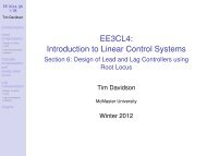
<strong>EE</strong> <strong>3CL4</strong>: <strong>Intro</strong>. <strong>to</strong> <strong>Linear</strong> <strong>Control</strong> <strong>Systems</strong><br />
<strong>Lab</strong> 3: <strong>Lead</strong> <strong>Compensation</strong><br />
Tim Davidson<br />
Ext. 27352<br />
davidson@mcmaster.ca<br />
Objective<br />
To use the root locus technique <strong>to</strong> design a lead compensa<strong>to</strong>r for a marginally-stable servomo<strong>to</strong>r.<br />
Assessment<br />
The assessment for this labora<strong>to</strong>ry will consist of<br />
1. a pre-lab design exercise, which must be completed before the lab,<br />
2. a system identification experiment,<br />
3. the design of a lead compensa<strong>to</strong>r for the system identified in item 2,<br />
4. an experiment <strong>to</strong> evaluate the performance of the compensated closed loop designed in item 3.<br />
Your answer <strong>to</strong> the pre-lab exercise will be evaluated at the beginning of the lab. Your performance of the<br />
system identification experiment, the compensa<strong>to</strong>r design and the performance evaluation experiment will<br />
be evaluated during the lab. The marks for each component are clearly indicated.<br />
1 Pre-lab design exercise (5 marks)<br />
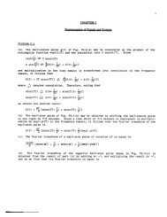
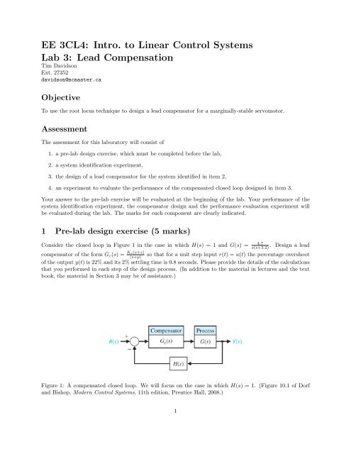
Consider the closed loop in Figure 1 in the case in which H(s) = 1 and G(s) = 4.7<br />
s(s+3.2) . Design a lead<br />
compensa<strong>to</strong>r of the form Gc(s) = Kc(s+z)<br />
(s+p) so that for a unit step input r(t) = u(t) the percentage overshoot<br />
of the output y(t) is 22% and its 2% settling time is 0.8 seconds. Please provide the details of the calculations<br />
that you performed in each step of the design process. (In addition <strong>to</strong> the material in lectures and the text<br />
book, the material in Section 3 may be of assistance.)<br />
Figure 1: A compensated closed loop. We will focus on the case in which H(s) = 1. (Figure 10.1 of Dorf<br />
and Bishop, Modern <strong>Control</strong> <strong>Systems</strong>, 11th edition, Prentice Hall, 2008.)<br />
1
2 Exp. 1: Closed Loop System Identification (2 marks)<br />
Recall that we will model the mo<strong>to</strong>r in the experiments using the transfer function<br />
A<br />
G(s) =<br />
. (1)<br />
s(sτm + 1)<br />
In order <strong>to</strong> perform the design component of this lab, we will need <strong>to</strong> obtain the A and τm for the mo<strong>to</strong>r<br />
that you will use in this labora<strong>to</strong>ry. Note that the values that you obtain may be different from those that<br />
you obtained in <strong>Lab</strong>. 1, even if you are using the same mo<strong>to</strong>r.<br />
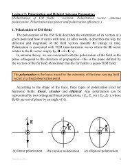
• Repeat experiments 1 and 2 from <strong>Lab</strong>. 1 <strong>to</strong> obtain the parameters A and τm for the mo<strong>to</strong>r that you<br />
will use in this labora<strong>to</strong>ry.<br />
• Remember that this involves constructing a circuit of the form in Fig. 2 using components in the form<br />
of Figs 3 and 4. For these systems you can choose R1 = R2 = 10 kΩ. Please follow the instructions<br />
from <strong>Lab</strong>. 1 carefully.<br />
To obtain your mark for this experiment you must show your TA the scope trace for input frequency ωp and<br />
must provide the corresponding values of A and τm.<br />
3 Design of a <strong>Lead</strong> Compensa<strong>to</strong>r for the Servomo<strong>to</strong>r<br />
In <strong>Lab</strong>. 2, we designed a proportional controller that had a large gain and achieved no more than 25%<br />
overshoot. However, we were unable <strong>to</strong> adjust the settling time of the closed loop by manipulating the value<br />
of the amplifier gain.<br />
In this lab, we will design a lead compensa<strong>to</strong>r that will enable us <strong>to</strong> achieve 25% overshoot and a settling<br />
time that is three times shorter than that achieved in <strong>Lab</strong>. 2. We will also examine the velocity error constant<br />
obtained in this design.<br />
3.1 Design of compensa<strong>to</strong>r (7 marks)<br />
In this section we will determine the pole positions required <strong>to</strong> achieve the desired goals.<br />
• Begin a sketch of the root locus by rewriting the mo<strong>to</strong>r transfer function as G(s) = A/τm<br />
s(s+1/τm) and<br />
plotting the poles of the model in (1).<br />
• Recall from <strong>Lab</strong>. 2 that the time constant for an underdamped closed loop with proportional control<br />
is 2τm.<br />
• On your graph, mark with squares the positions of the closed loop poles that would result in an<br />
overshoot of 25% and a settling time that is 1/3 of that achieved in the previous lab.<br />
• As a first step in the design of the compensa<strong>to</strong>r, Gc(s) = Kc s+z<br />
s+p , place the zero of the compensa<strong>to</strong>r on<br />
the real axis with the same real part as that of the desired closed-loop poles.<br />
• The pole of the compensa<strong>to</strong>r will be on the real axis <strong>to</strong> the left of this zero. Use the angle criterion <strong>to</strong><br />
determine where the pole should be placed in order for the root locus <strong>to</strong> pass through the squares.<br />
• Use the magnitude criterion <strong>to</strong> determine the gain KcA/τm required <strong>to</strong> place the poles in this position.<br />
• Complete the sketch of the root locus. You will need <strong>to</strong> compute the angles and the centroid of the<br />
asymp<strong>to</strong>tes, but you may simply estimate the breakaway points.<br />
2
Figure 2: Closed loop circuit from <strong>Lab</strong>s 1 and 2.<br />
Figure 3: Summing amplifier.<br />
Figure 4: Unit-gain inverting amplifier (inverter).<br />
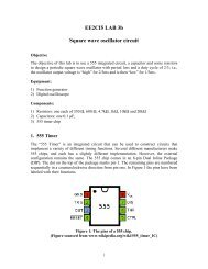
Figure 5: An implementation of a lead compensa<strong>to</strong>r.<br />
3
• If we write the compensa<strong>to</strong>r in the form Gc(s) = ˜ Kc aτs+1<br />
τs+1 what values should we choose for τ, a and<br />
˜Kc?<br />
• Compute the velocity error constant for the closed loop that you have designed. Recall that the velocity<br />
error constant of a stable closed loop satisfies 1<br />
Kv = lims→0 s 1<br />
1+Gc(s)G(s)<br />
To obtain your marks for this section, you must show a TA your worked solution, including the computed<br />
position for the pole, your sketch of the root locus, and the values you computed for τ, a and ˜ Kc<br />
3.2 Design of compensa<strong>to</strong>r circuit (3 marks)<br />
The goal of this section is <strong>to</strong> design a circuit that will implement the compensa<strong>to</strong>r that was designed in the<br />
previous section.<br />
• For the circuit in Fig. 5, assume that the op-amp is ideal and the bias resis<strong>to</strong>r is absent. Show that<br />
the transfer function can be written as<br />
Gc(s) = − ˜ aτs + 1<br />
Kc<br />
τs + 1<br />
where ˜ Kc = R3/R2, τ = C1R1, and a = (R1 + R2)/R1. Note that a > 1 so that the zero is closer <strong>to</strong><br />
the origin than the pole. Hence, this circuit can be used <strong>to</strong> construct a lead compensa<strong>to</strong>r.<br />
• Now choose values for R1, R2, R3 and C1 so that we achieve the desired value of ˜ Kc, and the zero and<br />
pole positions designed above. Note that there are three requirements, and four degrees of freedom.<br />
This provides the flexibility required <strong>to</strong> ensure that we can use standard values for at least some of the<br />
components. In particular,<br />
– Capaci<strong>to</strong>rs should be selected between 0.1µF and 30µF, preferably from standard values.<br />
– For the op-amps that we are using, resis<strong>to</strong>rs should be chosen between 10kΩ and 1MΩ. If R2 is<br />
chosen <strong>to</strong> be larger than 500kΩ, we must add the bias resis<strong>to</strong>r in Fig. 5.<br />
– As a guide, you should consider choosing R2 <strong>to</strong> be a value that satisfies 10 4 (a − 1) ≤ R2 ≤<br />
10 7 (a − 1), preferably a standard value. That should enable you <strong>to</strong> choose values for the capaci<strong>to</strong>r<br />
and R1 that can be constructed from the available equipment and enable linear operation of the<br />
op-amp.<br />
To obtain your marks for this section, you must show a TA your worked solution, including the values for<br />
the resis<strong>to</strong>rs and the capaci<strong>to</strong>r.<br />
4 Exp. 2: Implementation of the <strong>Lead</strong> Compensa<strong>to</strong>r<br />
4.1 Construct the closed loop (1 mark)<br />
Construct a closed loop that implements the designed system using a combination of the summing amplifier<br />
in Fig. 3, the inverter in Fig. 4, the lead compensa<strong>to</strong>r in Fig. 5, and the SEU. (Recall that the output of<br />
the summing amplifier is proportional <strong>to</strong> the negative of the sum.) Make sure that the Laplace Transform<br />
of the output of the compensa<strong>to</strong>r is Gc(s) � R(s) − Θ(s) � , where R(s) is the Laplace Transform of the input<br />
and Θ(s) is the Laplace Transform of the angle output. In order <strong>to</strong> ensure that the sign of this output is<br />
correct, the architecture of your closed loop may need <strong>to</strong> be different from that in Fig. 2.<br />
Before enabling this circuit, obtain your mark for this section by showing your block diagram <strong>to</strong> a TA, and<br />
showing the TA your implementation.<br />
4<br />
1<br />
s 2 .<br />
(2)
4.2 Evaluation of the design<br />
To obtain your marks for each section, you must show a TA the appropriate trace on the oscilloscope and<br />
your associated calculations, and you should provide appropriate discussion.<br />
4.2.1 Evaluate the percentage overshoot of your design (4 marks)<br />
Apply a square wave <strong>to</strong> the command input, and measure the percentage overshoot that you obtained. Make<br />
sure that the amplitude is large enough so that the non-linear effects of the mo<strong>to</strong>r are mitigated, but small<br />
enough so that the op-amp voltage does not saturate. Some guidance on the latter point can be obtained<br />
by considering the steady-state response of the compensa<strong>to</strong>r circuit <strong>to</strong> a step input, and the percentage<br />
overshoot.<br />
4.2.2 Evaluate the settling time of your design (4 marks)<br />
Apply a square wave <strong>to</strong> the command input, and assess the settling time. Compare this value <strong>to</strong> 8τm, which<br />
was the settling time of an underdamped closed-loop with proportional control.<br />
4.2.3 Evaluate the velocity error constant of your design (2 marks)<br />
Apply a triangular wave <strong>to</strong> the command input. Make sure that the frequency of the wave is low enough for<br />
the loop <strong>to</strong> settle in<strong>to</strong> the steady state before the wave reverses. Let β be the magnitude of the slope of the<br />
triangular wave. Estimate the velocity error constant by dividing the steady-state value of r(t) − θ(t) by β.<br />
The steady-state error can be measured by measuring the input r(t) using channel 1 of the oscilloscope and<br />
measuring the output θ(t) using channel 2. Be sure <strong>to</strong> select a value of β that facilitates this measurement.<br />
Compare the achieved velocity error constant <strong>to</strong> the value that can be calculated from the gains and the<br />
positions of the open-loop poles and zeros in your design in Section 3.1.<br />
5