Lead and Lag Compensator Design using Root Locus
Lead and Lag Compensator Design using Root Locus
Lead and Lag Compensator Design using Root Locus

Create successful ePaper yourself
Turn your PDF publications into a flip-book with our unique Google optimized e-Paper software.
EE 3CL4, §6<br />
1 / 38<br />
Tim Davidson<br />
<strong>Compensator</strong>s<br />
<strong>Lead</strong><br />
compensation<br />
<strong>Design</strong> via <strong>Root</strong><br />
<strong>Locus</strong><br />
<strong>Lead</strong> <strong>Compensator</strong><br />
example<br />
Cascade<br />
compensation<br />
<strong>and</strong><br />
steady-state<br />
errors<br />
<strong>Lag</strong><br />
Compensation<br />
<strong>Design</strong> via <strong>Root</strong><br />
<strong>Locus</strong><br />
<strong>Lag</strong> compensator<br />
example<br />
Insights<br />
EE3CL4:<br />
Introduction to Linear Control Systems<br />
Section 6: <strong>Design</strong> of <strong>Lead</strong> <strong>and</strong> <strong>Lag</strong> Controllers <strong>using</strong><br />
<strong>Root</strong> <strong>Locus</strong><br />
Tim Davidson<br />
McMaster University<br />
Winter 2012
EE 3CL4, §6<br />
2 / 38<br />
Tim Davidson<br />
<strong>Compensator</strong>s<br />
<strong>Lead</strong><br />
compensation<br />
<strong>Design</strong> via <strong>Root</strong><br />
<strong>Locus</strong><br />
<strong>Lead</strong> <strong>Compensator</strong><br />
example<br />
Cascade<br />
compensation<br />
<strong>and</strong><br />
steady-state<br />
errors<br />
<strong>Lag</strong><br />
Compensation<br />
<strong>Design</strong> via <strong>Root</strong><br />
<strong>Locus</strong><br />
<strong>Lag</strong> compensator<br />
example<br />
Insights<br />
1 <strong>Compensator</strong>s<br />
2 <strong>Lead</strong> compensation<br />
<strong>Design</strong> via <strong>Root</strong> <strong>Locus</strong><br />
<strong>Lead</strong> <strong>Compensator</strong> example<br />
Outline<br />
3 Cascade compensation <strong>and</strong> steady-state errors<br />
4 <strong>Lag</strong> Compensation<br />
<strong>Design</strong> via <strong>Root</strong> <strong>Locus</strong><br />
<strong>Lag</strong> compensator example<br />
5 Insights
EE 3CL4, §6<br />
4 / 38<br />
Tim Davidson<br />
<strong>Compensator</strong>s<br />
<strong>Lead</strong><br />
compensation<br />
<strong>Design</strong> via <strong>Root</strong><br />
<strong>Locus</strong><br />
<strong>Lead</strong> <strong>Compensator</strong><br />
example<br />
Cascade<br />
compensation<br />
<strong>and</strong><br />
steady-state<br />
errors<br />
<strong>Lag</strong><br />
Compensation<br />
<strong>Design</strong> via <strong>Root</strong><br />
<strong>Locus</strong><br />
<strong>Lag</strong> compensator<br />
example<br />
Insights<br />
<strong>Compensator</strong>s<br />
• Early in the course we provided some useful guidelines<br />
regarding the relationships between the pole positions<br />
of a system <strong>and</strong> certain aspects of its performance<br />
• Using root locus techniques, we have seen how the<br />
pole positions of a closed loop can be adjusted by<br />
varying a parameter<br />
• What happens if we are unable to obtain that<br />
performance that we want by doing this?<br />
• Ask ourselves whether this is really the performance<br />
that we want<br />
• Ask whether we can change the system,<br />
say by buying different components<br />
• seek to compensate for the undesirable aspects of the<br />
process
EE 3CL4, §6<br />
5 / 38<br />
Tim Davidson<br />
<strong>Compensator</strong>s<br />
<strong>Lead</strong><br />
compensation<br />
<strong>Design</strong> via <strong>Root</strong><br />
<strong>Locus</strong><br />
<strong>Lead</strong> <strong>Compensator</strong><br />
example<br />
Cascade<br />
compensation<br />
<strong>and</strong><br />
steady-state<br />
errors<br />
<strong>Lag</strong><br />
Compensation<br />
<strong>Design</strong> via <strong>Root</strong><br />
<strong>Locus</strong><br />
<strong>Lag</strong> compensator<br />
example<br />
Insights<br />
Cascade compensation<br />
• Usually, the plant is a physical process<br />
• If comm<strong>and</strong>s <strong>and</strong> measurements are made electrically,<br />
compensator is often an electric circuit<br />
• General form of the compensator is<br />
Gc(s) = Kc<br />
�M i=1 (s + zi)<br />
�n j=1 (s + pj)<br />
• Therefore, the cascade compensator adds open loop<br />
poles <strong>and</strong> open loop zeros<br />
• These will change the shape of the root locus
EE 3CL4, §6<br />
6 / 38<br />
Tim Davidson<br />
<strong>Compensator</strong>s<br />
<strong>Lead</strong><br />
compensation<br />
<strong>Design</strong> via <strong>Root</strong><br />
<strong>Locus</strong><br />
<strong>Lead</strong> <strong>Compensator</strong><br />
example<br />
Cascade<br />
compensation<br />
<strong>and</strong><br />
steady-state<br />
errors<br />
<strong>Lag</strong><br />
Compensation<br />
<strong>Design</strong> via <strong>Root</strong><br />
<strong>Locus</strong><br />
<strong>Lag</strong> compensator<br />
example<br />
Insights<br />
<strong>Compensator</strong> design<br />
• Where should we put new poles <strong>and</strong> zeros to achieve<br />
desired performance?<br />
• That is the art of compensator design<br />
• We will consider first order compensators of the form<br />
Gc(s) = Kc(s + z)<br />
(s + p) = ˜ Kc(1 + s/z)<br />
(1 + s/p) , where ˜ Kc = Kcz/p<br />
• with the pole −p in the left half plane<br />
• <strong>and</strong> the zero, −z in the left half plane, too<br />
• For reasons that will soon become clear<br />
• when |z| < |p|: phase lead network<br />
• when |z| > |p|: phase lag network
EE 3CL4, §6<br />
8 / 38<br />
Tim Davidson<br />
<strong>Compensator</strong>s<br />
<strong>Lead</strong><br />
compensation<br />
<strong>Design</strong> via <strong>Root</strong><br />
<strong>Locus</strong><br />
<strong>Lead</strong> <strong>Compensator</strong><br />
example<br />
Cascade<br />
compensation<br />
<strong>and</strong><br />
steady-state<br />
errors<br />
<strong>Lag</strong><br />
Compensation<br />
<strong>Design</strong> via <strong>Root</strong><br />
<strong>Locus</strong><br />
<strong>Lag</strong> compensator<br />
example<br />
Insights<br />
<strong>Lead</strong> compensation<br />
Gc(s) = Kc(s + z)<br />
(s + p)<br />
with |z| < |p|. That is, zero closer to origin than pole<br />
Let p = 1/τ <strong>and</strong> z = 1/(αleadτ). Since z < p, αlead > 1.<br />
Define ˜ Kc = Kcz/p = Kc/αlead. Then<br />
Gc(s) = Kc(s + z)<br />
(s + p) = ˜ Kc(1 + αleadτs)<br />
(1 + τs)
EE 3CL4, §6<br />
9 / 38<br />
Tim Davidson<br />
<strong>Compensator</strong>s<br />
<strong>Lead</strong><br />
compensation<br />
<strong>Design</strong> via <strong>Root</strong><br />
<strong>Locus</strong><br />
<strong>Lead</strong> <strong>Compensator</strong><br />
example<br />
Cascade<br />
compensation<br />
<strong>and</strong><br />
steady-state<br />
errors<br />
<strong>Lag</strong><br />
Compensation<br />
<strong>Design</strong> via <strong>Root</strong><br />
<strong>Locus</strong><br />
<strong>Lag</strong> compensator<br />
example<br />
Insights<br />
<strong>Lead</strong> compensation<br />
With |z| < |p|, αlead > 1, Gc(s) = Kc(s+z)<br />
(s+p) = ˜ Kc(1+αleadτs) (1+τs)<br />
• Frequency response:<br />
• Bode diagram<br />
Gc(jω) = ˜ Kc(1 + jωαleadτ)<br />
(1 + jωτ)<br />
• Between ω = z <strong>and</strong> ω = p, |Gc(jω)| ≈ ˜ Kcωαleadτ<br />
• What kind of operator has a frequency response with<br />
magnitude proportional to ω? Differentiator<br />
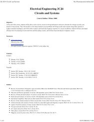
• Note that the phase is positive. Hence “phase lead”
EE 3CL4, §6<br />
10 / 38<br />
Tim Davidson<br />
<strong>Compensator</strong>s<br />
<strong>Lead</strong><br />
compensation<br />
<strong>Design</strong> via <strong>Root</strong><br />
<strong>Locus</strong><br />
<strong>Lead</strong> <strong>Compensator</strong><br />
example<br />
Cascade<br />
compensation<br />
<strong>and</strong><br />
steady-state<br />
errors<br />
<strong>Lag</strong><br />
Compensation<br />
<strong>Design</strong> via <strong>Root</strong><br />
<strong>Locus</strong><br />
<strong>Lag</strong> compensator<br />
example<br />
Insights<br />
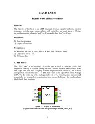
A passive phase lead network<br />
Homework: Show that V 2(s)<br />
V 1(s) has the phase lead<br />
characteristic
EE 3CL4, §6<br />
11 / 38<br />
Tim Davidson<br />
<strong>Compensator</strong>s<br />
<strong>Lead</strong><br />
compensation<br />
<strong>Design</strong> via <strong>Root</strong><br />
<strong>Locus</strong><br />
<strong>Lead</strong> <strong>Compensator</strong><br />
example<br />
Cascade<br />
compensation<br />
<strong>and</strong><br />
steady-state<br />
errors<br />
<strong>Lag</strong><br />
Compensation<br />
<strong>Design</strong> via <strong>Root</strong><br />
<strong>Locus</strong><br />
<strong>Lag</strong> compensator<br />
example<br />
Insights<br />
Active lead <strong>and</strong> lag networks<br />
Here’s an example of an active network architecture.
EE 3CL4, §6<br />
12 / 38<br />
Tim Davidson<br />
<strong>Compensator</strong>s<br />
<strong>Lead</strong><br />
compensation<br />
<strong>Design</strong> via <strong>Root</strong><br />
<strong>Locus</strong><br />
<strong>Lead</strong> <strong>Compensator</strong><br />
example<br />
Cascade<br />
compensation<br />
<strong>and</strong><br />
steady-state<br />
errors<br />
<strong>Lag</strong><br />
Compensation<br />
<strong>Design</strong> via <strong>Root</strong><br />
<strong>Locus</strong><br />
<strong>Lag</strong> compensator<br />
example<br />
Insights<br />
Principles of <strong>Lead</strong> design via<br />
<strong>Root</strong> <strong>Locus</strong><br />
• The compensator adds poles <strong>and</strong> zeros to the P(s) in<br />
the root locus procedure.<br />
• Hence we can change the shape of the root locus.<br />
• If we can capture desirable performance in terms of<br />
positions of closed loop poles<br />
• then compensator design problem reduces to:<br />
• changing the shape of the root locus so that these<br />
desired closed-loop pole positions appear on the root<br />
locus<br />
• finding the gain that places the closed-loop pole<br />
positions at their desired positions<br />
• What tools do we have to do this?<br />
• Phase criterion <strong>and</strong> magnitude criterion, respectively
EE 3CL4, §6<br />
13 / 38<br />
Tim Davidson<br />
<strong>Compensator</strong>s<br />
<strong>Lead</strong><br />
compensation<br />
<strong>Design</strong> via <strong>Root</strong><br />
<strong>Locus</strong><br />
<strong>Lead</strong> <strong>Compensator</strong><br />
example<br />
Cascade<br />
compensation<br />
<strong>and</strong><br />
steady-state<br />
errors<br />
<strong>Lag</strong><br />
Compensation<br />
<strong>Design</strong> via <strong>Root</strong><br />
<strong>Locus</strong><br />
<strong>Lag</strong> compensator<br />
example<br />
Insights<br />
<strong>Root</strong> <strong>Locus</strong> Principles<br />
• The point s0 is on the root locus of P(s) if 1 + KP(s0) = 0.<br />
• In first order compensator design with G(s) = K G<br />
<strong>and</strong> Gc = Kc(s+z)<br />
(s+z)<br />
(s+p) , we have P(s) = (s+p)<br />
QM i=1 (s+zi )<br />
Qn j=1 (s+pj )<br />
Q M<br />
i=1 (s+zi )<br />
Q n<br />
j=1 (s+pj ) <strong>and</strong><br />
K = KcKG. We will restrict attention to the case of K > 0<br />
• Phase cond. s0 is on root locus if ∠P(s0) = 180 ◦ + k360 ◦ :<br />
M�<br />
(angle from −zi to s0) −<br />
i=1<br />
n�<br />
(angle from −pj to s0)<br />
j=1<br />
+ (angle from −z to s0) − (angle from −p to s0)<br />
= 180 ◦ + k 360 ◦<br />
• Mag. cond. If s0 satisfies phase condition, the gain that puts<br />
a closed-loop pole at s0 is K = 1/|P(s0)|:<br />
�n j=1<br />
K =<br />
(dist from −pj to s0)<br />
�M i=1 (dist from −zi<br />
(dist from −p to s0)<br />
×<br />
to s0) (dist from −z to s0)
EE 3CL4, §6<br />
14 / 38<br />
Tim Davidson<br />
<strong>Compensator</strong>s<br />
<strong>Lead</strong><br />
compensation<br />
<strong>Design</strong> via <strong>Root</strong><br />
<strong>Locus</strong><br />
<strong>Lead</strong> <strong>Compensator</strong><br />
example<br />
Cascade<br />
compensation<br />
<strong>and</strong><br />
steady-state<br />
errors<br />
<strong>Lag</strong><br />
Compensation<br />
<strong>Design</strong> via <strong>Root</strong><br />
<strong>Locus</strong><br />
<strong>Lag</strong> compensator<br />
example<br />
Insights<br />
RL design: Basic procedure<br />
1 Translate design specifications into desired positions of<br />
dominant poles<br />
2 Sketch root locus of uncompensated system to see if desired<br />
positions can be achieved<br />
3 If not, choose the positions of the pole <strong>and</strong> zero of the<br />
compensator so that the desired positions lie on the root<br />
locus (phase criterion), if that is possible<br />
4 Evaluate the gain required to put the poles there<br />
(magnitude criterion)<br />
5 Evaluate the total system gain so that the steady-state error<br />
constants can be determined<br />
6 If the steady state error constants are not satisfactory, repeat<br />
This procedure enables relatively straightforward design of<br />
systems with specifications in terms of rise time, settling time, <strong>and</strong><br />
overshoot; i.e., the transient response.<br />
For systems with steady-state error specifications, Bode (<strong>and</strong><br />
Nyquist) methods may be more straightforward (later)
EE 3CL4, §6<br />
15 / 38<br />
Tim Davidson<br />
<strong>Compensator</strong>s<br />
<strong>Lead</strong><br />
compensation<br />
<strong>Design</strong> via <strong>Root</strong><br />
<strong>Locus</strong><br />
<strong>Lead</strong> <strong>Compensator</strong><br />
example<br />
Cascade<br />
compensation<br />
<strong>and</strong><br />
steady-state<br />
errors<br />
<strong>Lag</strong><br />
Compensation<br />
<strong>Design</strong> via <strong>Root</strong><br />
<strong>Locus</strong><br />
<strong>Lag</strong> compensator<br />
example<br />
Insights<br />
<strong>Lead</strong> Comp. example<br />
Consider a case with G(s) = 1<br />
s(s+2) <strong>and</strong> H(s) = 1.<br />
<strong>Design</strong> a lead compensator to achieve:<br />
• damping coefficient ζ = 0.45 <strong>and</strong><br />
• velocity error constant Kv = lims→0 sGc(s)G(s) > 20<br />
What to do?<br />
• Let’s draw something. Plot poles of G(s).<br />
Where should the closed-loop poles be? cos −1 (0.45) ≈ 64 ◦<br />
• Note that the settling time is not specified. We are free to<br />
choose it. However, we need a large Kv which will require<br />
large gain. Need desired positions far from open loop poles.<br />
• Let’s start with desired roots ≈ −4 ± j8<br />
• This pair has Ts = 1 <strong>and</strong> ωn ≈ 9
EE 3CL4, §6<br />
16 / 38<br />
Tim Davidson<br />
<strong>Compensator</strong>s<br />
<strong>Lead</strong><br />
compensation<br />
<strong>Design</strong> via <strong>Root</strong><br />
<strong>Locus</strong><br />
<strong>Lead</strong> <strong>Compensator</strong><br />
example<br />
Cascade<br />
compensation<br />
<strong>and</strong><br />
steady-state<br />
errors<br />
<strong>Lag</strong><br />
Compensation<br />
<strong>Design</strong> via <strong>Root</strong><br />
<strong>Locus</strong><br />
<strong>Lag</strong> compensator<br />
example<br />
Insights<br />
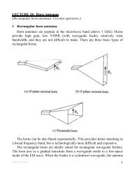
<strong>Lead</strong> Comp. example<br />
• Now where to put the zero <strong>and</strong> pole?<br />
• Rule of thumb: put zero under desired root, or just to the left<br />
• Determine position of the pole <strong>using</strong> angle criterion<br />
sum angles from open-loop zeros<br />
• Hence pole at ≈ −10.6<br />
• Gain of compensated system:<br />
− sum angles from open-loop poles = 180 ◦<br />
90 − (116 + 104 + θp) = 180<br />
=⇒ θp = 50<br />
Prod. dist. from open-loop poles 9(8.25)(10.4)<br />
≈ = 96.5<br />
Prod. dist. from open-loop zeros 8<br />
• Hence compensated open loop: Gc(s)G(s) = 96.5(s+4)<br />
s(s+2)(s+10.6)<br />
• Velocity constant: Kv = lims→0 sGc(s)G(s) = 18.2 :(
EE 3CL4, §6<br />
17 / 38<br />
Tim Davidson<br />
<strong>Compensator</strong>s<br />
<strong>Lead</strong><br />
compensation<br />
<strong>Design</strong> via <strong>Root</strong><br />
<strong>Locus</strong><br />
<strong>Lead</strong> <strong>Compensator</strong><br />
example<br />
Cascade<br />
compensation<br />
<strong>and</strong><br />
steady-state<br />
errors<br />
<strong>Lag</strong><br />
Compensation<br />
<strong>Design</strong> via <strong>Root</strong><br />
<strong>Locus</strong><br />
<strong>Lag</strong> compensator<br />
example<br />
Insights<br />
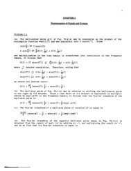
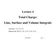
Compensated root locus<br />
<strong>Root</strong> locus <strong>and</strong> the step response with the dominant roots at<br />
their desired locations
EE 3CL4, §6<br />
18 / 38<br />
Tim Davidson<br />
<strong>Compensator</strong>s<br />
<strong>Lead</strong><br />
compensation<br />
<strong>Design</strong> via <strong>Root</strong><br />
<strong>Locus</strong><br />
<strong>Lead</strong> <strong>Compensator</strong><br />
example<br />
Cascade<br />
compensation<br />
<strong>and</strong><br />
steady-state<br />
errors<br />
<strong>Lag</strong><br />
Compensation<br />
<strong>Design</strong> via <strong>Root</strong><br />
<strong>Locus</strong><br />
<strong>Lag</strong> compensator<br />
example<br />
Insights<br />
What to do now?<br />
• We tried hard, but did not achieve the design specs<br />
• Let’s go back <strong>and</strong> re-examine our choices<br />
• Zero position of compensator was chosen via rule of<br />
thumb<br />
• Can we do better?<br />
Yes, but two parameter design becomes trickier.<br />
• What were other choices that we made?<br />
• We chose desired poles to be of magnitude ωn ≈ 9<br />
• We could choose them to be further away<br />
(faster transient response)<br />
• By how much?<br />
• Show that when desired poles have ωn = 10 as well as<br />
the required ζ = 0.45, then the choice of z = 4.5,<br />
p = 11.6 <strong>and</strong> the corresp. Kc results in Kv = 22.7
EE 3CL4, §6<br />
19 / 38<br />
Tim Davidson<br />
<strong>Compensator</strong>s<br />
<strong>Lead</strong><br />
compensation<br />
<strong>Design</strong> via <strong>Root</strong><br />
<strong>Locus</strong><br />
<strong>Lead</strong> <strong>Compensator</strong><br />
example<br />
Cascade<br />
compensation<br />
<strong>and</strong><br />
steady-state<br />
errors<br />
<strong>Lag</strong><br />
Compensation<br />
<strong>Design</strong> via <strong>Root</strong><br />
<strong>Locus</strong><br />
<strong>Lag</strong> compensator<br />
example<br />
Insights<br />
Outcomes<br />
• <strong>Root</strong> locus approach to phase lead design was<br />
reasonably successful in terms of putting dominant<br />
poles in desired positions; e.g., in terms of ζ <strong>and</strong> ωn<br />
• We did this by positioning the pole <strong>and</strong> zero of the lead<br />
compensator so as to change the shape of the root<br />
locus<br />
• However, root locus approach does not provide<br />
independent control over steady-state error constants<br />
(details upcoming)<br />
• That said, since lead compensators reduce the DC gain<br />
(they resemble differentiators), they are not normally<br />
used to control steady-state error.<br />
• The goal of our lag compensator design will be to<br />
increase the steady-state error constants, without<br />
moving the other poles too far
EE 3CL4, §6<br />
21 / 38<br />
Tim Davidson<br />
<strong>Compensator</strong>s<br />
<strong>Lead</strong><br />
compensation<br />
<strong>Design</strong> via <strong>Root</strong><br />
<strong>Locus</strong><br />
<strong>Lead</strong> <strong>Compensator</strong><br />
example<br />
Cascade<br />
compensation<br />
<strong>and</strong><br />
steady-state<br />
errors<br />
<strong>Lag</strong><br />
Compensation<br />
<strong>Design</strong> via <strong>Root</strong><br />
<strong>Locus</strong><br />
<strong>Lag</strong> compensator<br />
example<br />
Insights<br />
Cascade compensation<br />
• Throughout this lecture, <strong>and</strong> all the discussion on cascade<br />
compensation, we will consider the case in which H(s) = 1.<br />
• We will consider first order compensators of the form<br />
Gc(s) =<br />
K (s + z)<br />
(s + p)<br />
with the pole, −p, <strong>and</strong> the zero, −z, both in the left half plane<br />
• when |z| < |p|: phase lead network<br />
• when |z| > |p|: phase lag network
EE 3CL4, §6<br />
22 / 38<br />
Tim Davidson<br />
<strong>Compensator</strong>s<br />
<strong>Lead</strong><br />
compensation<br />
<strong>Design</strong> via <strong>Root</strong><br />
<strong>Locus</strong><br />
<strong>Lead</strong> <strong>Compensator</strong><br />
example<br />
Cascade<br />
compensation<br />
<strong>and</strong><br />
steady-state<br />
errors<br />
<strong>Lag</strong><br />
Compensation<br />
<strong>Design</strong> via <strong>Root</strong><br />
<strong>Locus</strong><br />
<strong>Lag</strong> compensator<br />
example<br />
Insights<br />
Steady-state errors<br />
If closed loop stable, steady state error for input R(s):<br />
Let G(s) = K G<br />
R(s)<br />
ess = lim e(t) = lim s<br />
t→∞ s→0 1 + GC(s)G(s)<br />
Q<br />
i (s+zi )<br />
Q<br />
j (s+pj ) <strong>and</strong> consider GC(s) = KC(s+z) (s+p)<br />
• Consider the case in which G(s) is a type-0 system.<br />
• Steady state error due to a step r(t) = Au(t):<br />
ess = A<br />
1+Kposn<br />
, where<br />
Kposn = GC(0)G(0) = KCz<br />
p<br />
• Note that for a lead compensator, z/p < 1,<br />
�<br />
KG i zi<br />
�<br />
j pj<br />
• So lead compensation may degrade steady-state error<br />
performance
EE 3CL4, §6<br />
23 / 38<br />
Tim Davidson<br />
<strong>Compensator</strong>s<br />
<strong>Lead</strong><br />
compensation<br />
<strong>Design</strong> via <strong>Root</strong><br />
<strong>Locus</strong><br />
<strong>Lead</strong> <strong>Compensator</strong><br />
example<br />
Cascade<br />
compensation<br />
<strong>and</strong><br />
steady-state<br />
errors<br />
<strong>Lag</strong><br />
Compensation<br />
<strong>Design</strong> via <strong>Root</strong><br />
<strong>Locus</strong><br />
<strong>Lag</strong> compensator<br />
example<br />
Insights<br />
Steady-state error<br />
• Now, consider the case in which G(s) is a type-1<br />
system, G(s) = K Q<br />
G i (s+zi )<br />
s Q<br />
j (s+pj )<br />
• Steady-state error due to a ramp r(t) = At: ess = A/Kv,<br />
where the velocity constant is<br />
Kv = lim<br />
s→0 sGc(s)G(s) = K Cz<br />
p<br />
�<br />
KG i zi<br />
�<br />
j pj<br />
• Once again, lead compensation may degrade<br />
steady-state error performance<br />
• Is there a way to increase the value of these error<br />
constants while leaving the closed loop poles in<br />
essentially the same place as they were in an<br />
uncompensated system? Perhaps |z| > |p|?
EE 3CL4, §6<br />
25 / 38<br />
Tim Davidson<br />
<strong>Compensator</strong>s<br />
<strong>Lead</strong><br />
compensation<br />
<strong>Design</strong> via <strong>Root</strong><br />
<strong>Locus</strong><br />
<strong>Lead</strong> <strong>Compensator</strong><br />
example<br />
Cascade<br />
compensation<br />
<strong>and</strong><br />
steady-state<br />
errors<br />
<strong>Lag</strong><br />
Compensation<br />
<strong>Design</strong> via <strong>Root</strong><br />
<strong>Locus</strong><br />
<strong>Lag</strong> compensator<br />
example<br />
Insights<br />
<strong>Lag</strong> compensation<br />
Gc(s) = Kc(s + z)<br />
(s + p)<br />
with |z| > |p|. That is, pole closer to origin than zero<br />
Let z = 1/τ <strong>and</strong> p = 1/(αlagτ). Since z > p, αlag > 1.<br />
Define ˜ Kc = Kcz/p = Kcαlag. Then<br />
Gc(s) = Kc(s + z)<br />
(s + p) = ˜ Kc(1 + τs)<br />
(1 + αlagτs)
EE 3CL4, §6<br />
26 / 38<br />
Tim Davidson<br />
<strong>Compensator</strong>s<br />
<strong>Lead</strong><br />
compensation<br />
<strong>Design</strong> via <strong>Root</strong><br />
<strong>Locus</strong><br />
<strong>Lead</strong> <strong>Compensator</strong><br />
example<br />
Cascade<br />
compensation<br />
<strong>and</strong><br />
steady-state<br />
errors<br />
<strong>Lag</strong><br />
Compensation<br />
<strong>Design</strong> via <strong>Root</strong><br />
<strong>Locus</strong><br />
<strong>Lag</strong> compensator<br />
example<br />
Insights<br />
Magnitude<br />
Frequency response<br />
Gc(jω) = ˜ K C(1 + jωτ)<br />
(1 + jωαlagτ)<br />
• Low frequency gain: ˜ K C<br />
• Corner frequency in denominator at ωp = p = 1/(αlagτ)<br />
• Corner frequency in numerator at ωz = z = 1/τ<br />
• ωp < ωz<br />
• High frequency gain: ˜ K C/αlag = K C<br />
Phase<br />
• φ(ω) = atan(ωτ) − atan(αlagωτ)<br />
• At low frequency: φ(ω) = 0<br />
• At high frequency: φ(ω) = 0<br />
• In between: negative, with max. lag at ω = √ zp
EE 3CL4, §6<br />
27 / 38<br />
Tim Davidson<br />
<strong>Compensator</strong>s<br />
<strong>Lead</strong><br />
compensation<br />
<strong>Design</strong> via <strong>Root</strong><br />
<strong>Locus</strong><br />
<strong>Lead</strong> <strong>Compensator</strong><br />
example<br />
Cascade<br />
compensation<br />
<strong>and</strong><br />
steady-state<br />
errors<br />
<strong>Lag</strong><br />
Compensation<br />
<strong>Design</strong> via <strong>Root</strong><br />
<strong>Locus</strong><br />
<strong>Lag</strong> compensator<br />
example<br />
Insights<br />
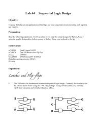
Note integrative characteristic<br />
Bode Diagram
EE 3CL4, §6<br />
28 / 38<br />
Tim Davidson<br />
<strong>Compensator</strong>s<br />
<strong>Lead</strong><br />
compensation<br />
<strong>Design</strong> via <strong>Root</strong><br />
<strong>Locus</strong><br />
<strong>Lead</strong> <strong>Compensator</strong><br />
example<br />
Cascade<br />
compensation<br />
<strong>and</strong><br />
steady-state<br />
errors<br />
<strong>Lag</strong><br />
Compensation<br />
<strong>Design</strong> via <strong>Root</strong><br />
<strong>Locus</strong><br />
<strong>Lag</strong> compensator<br />
example<br />
Insights<br />
A passive phase lag network
EE 3CL4, §6<br />
29 / 38<br />
Tim Davidson<br />
<strong>Compensator</strong>s<br />
<strong>Lead</strong><br />
compensation<br />
<strong>Design</strong> via <strong>Root</strong><br />
<strong>Locus</strong><br />
<strong>Lead</strong> <strong>Compensator</strong><br />
example<br />
Cascade<br />
compensation<br />
<strong>and</strong><br />
steady-state<br />
errors<br />
<strong>Lag</strong><br />
Compensation<br />
<strong>Design</strong> via <strong>Root</strong><br />
<strong>Locus</strong><br />
<strong>Lag</strong> compensator<br />
example<br />
Insights<br />
Active lead <strong>and</strong> lag networks<br />
Here’s an example of an active network architecture.
EE 3CL4, §6<br />
30 / 38<br />
Tim Davidson<br />
<strong>Compensator</strong>s<br />
<strong>Lead</strong><br />
compensation<br />
<strong>Design</strong> via <strong>Root</strong><br />
<strong>Locus</strong><br />
<strong>Lead</strong> <strong>Compensator</strong><br />
example<br />
Cascade<br />
compensation<br />
<strong>and</strong><br />
steady-state<br />
errors<br />
<strong>Lag</strong><br />
Compensation<br />
<strong>Design</strong> via <strong>Root</strong><br />
<strong>Locus</strong><br />
<strong>Lag</strong> compensator<br />
example<br />
Insights<br />
<strong>Lag</strong> compensator design<br />
• <strong>Lag</strong> compensator: Gc(s) = Kc s+z<br />
s+p . with |z| > |p|.<br />
• Recall position error constant for compensated type-0<br />
system <strong>and</strong> velocity error constant for compensated type-1<br />
system:<br />
Kposn = KCz<br />
p<br />
�<br />
KG i zi<br />
�<br />
j pj<br />
, Kv = KCz<br />
p<br />
�<br />
KG i zi<br />
�<br />
j pj<br />
where in the latter case the product in the denominator is<br />
over the non-zero poles.<br />
<strong>Design</strong> Principles<br />
• We don’t try to reshape the uncompensated root locus.<br />
• We just try to increase the value of the desired error constant<br />
by a factor αlag = z/p without moving the poles (well not<br />
much)<br />
• Reshaping was the goal of lead compensator design
EE 3CL4, §6<br />
31 / 38<br />
Tim Davidson<br />
<strong>Compensator</strong>s<br />
<strong>Lead</strong><br />
compensation<br />
<strong>Design</strong> via <strong>Root</strong><br />
<strong>Locus</strong><br />
<strong>Lead</strong> <strong>Compensator</strong><br />
example<br />
Cascade<br />
compensation<br />
<strong>and</strong><br />
steady-state<br />
errors<br />
<strong>Lag</strong><br />
Compensation<br />
<strong>Design</strong> via <strong>Root</strong><br />
<strong>Locus</strong><br />
<strong>Lag</strong> compensator<br />
example<br />
Insights<br />
<strong>Lag</strong> compensator design<br />
<strong>Design</strong> principles:<br />
• Don’t reshape the root locus<br />
• Adding the open loop pole <strong>and</strong> zero from the<br />
compensator should only result in a small change to the<br />
angle criterion for any point on the uncompensated root<br />
locus<br />
• Angles from compensator pole <strong>and</strong> zero to any point on<br />
the locus must be similar<br />
• Pole <strong>and</strong> zero must be close together<br />
• Increase value of error constant:<br />
• Want to have a large value for αlag = z/p.<br />
• How can that happen if z <strong>and</strong> p are close together?<br />
• Only if z <strong>and</strong> p are both small, i.e., close to the origin
EE 3CL4, §6<br />
32 / 38<br />
Tim Davidson<br />
<strong>Compensator</strong>s<br />
<strong>Lead</strong><br />
compensation<br />
<strong>Design</strong> via <strong>Root</strong><br />
<strong>Locus</strong><br />
<strong>Lead</strong> <strong>Compensator</strong><br />
example<br />
Cascade<br />
compensation<br />
<strong>and</strong><br />
steady-state<br />
errors<br />
<strong>Lag</strong><br />
Compensation<br />
<strong>Design</strong> via <strong>Root</strong><br />
<strong>Locus</strong><br />
<strong>Lag</strong> compensator<br />
example<br />
Insights<br />
<strong>Lag</strong> comp. design via <strong>Root</strong><br />
<strong>Locus</strong><br />
1 Obtain the root locus of uncompensated system<br />
2 From transient performance specs, locate suitable<br />
dominant pole positions on that locus<br />
3 Obtain the loop gain for these points, K = KPK G;<br />
hence the (closed-loop) steady-state error constant<br />
4 Calculate the necessary increase. Hence αlag = z/p<br />
5 Place pole <strong>and</strong> zero close to the origin (with respect to<br />
desired pole positions), with z = αlagp.<br />
Typically, choose z <strong>and</strong> p so that their angles to desired<br />
poles differ by less than 1 ◦ .<br />
6 Set Kc = KP<br />
What if there is nothing suitable at step 2?<br />
• Perhaps do lead compensation first,<br />
• then lag compensation on lead compensated plant.<br />
i.e., design a lead-lag compensator
EE 3CL4, §6<br />
33 / 38<br />
Tim Davidson<br />
<strong>Compensator</strong>s<br />
<strong>Lead</strong><br />
compensation<br />
<strong>Design</strong> via <strong>Root</strong><br />
<strong>Locus</strong><br />
<strong>Lead</strong> <strong>Compensator</strong><br />
example<br />
Cascade<br />
compensation<br />
<strong>and</strong><br />
steady-state<br />
errors<br />
<strong>Lag</strong><br />
Compensation<br />
<strong>Design</strong> via <strong>Root</strong><br />
<strong>Locus</strong><br />
<strong>Lag</strong> compensator<br />
example<br />
Insights<br />
Example<br />
Let’s consider, again, the case with G(s) = 1<br />
s(s+2) .<br />
<strong>Design</strong> a lag compensator to achieve damping coefficient<br />
ζ = 0.45 <strong>and</strong> velocity error constant Kv > 20<br />
Note: we will get a different closed loop from our lead<br />
design.<br />
First step, obtain uncompensated root locus, <strong>and</strong> locate<br />
desired dominant pole locations
EE 3CL4, §6<br />
34 / 38<br />
Tim Davidson<br />
<strong>Compensator</strong>s<br />
<strong>Lead</strong><br />
compensation<br />
<strong>Design</strong> via <strong>Root</strong><br />
<strong>Locus</strong><br />
<strong>Lead</strong> <strong>Compensator</strong><br />
example<br />
Cascade<br />
compensation<br />
<strong>and</strong><br />
steady-state<br />
errors<br />
<strong>Lag</strong><br />
Compensation<br />
<strong>Design</strong> via <strong>Root</strong><br />
<strong>Locus</strong><br />
<strong>Lag</strong> compensator<br />
example<br />
Insights<br />
Example<br />
• Gain required to put closed loop poles in desired position =<br />
prod. distances from open loop poles<br />
• That is, K = 2.24 2 = 5. Therefore KP = K /KG = 5<br />
• Velocity error const: Kv,unc = lims→0 sKPG(s) = K /2 = 2.5<br />
• The increase required is 20/2.5 = 8<br />
• That implies must choose p = z/8, where z is chosen to be<br />
close to the origin with respect to dominant closed-loop poles
EE 3CL4, §6<br />
35 / 38<br />
Tim Davidson<br />
<strong>Compensator</strong>s<br />
<strong>Lead</strong><br />
compensation<br />
<strong>Design</strong> via <strong>Root</strong><br />
<strong>Locus</strong><br />
<strong>Lead</strong> <strong>Compensator</strong><br />
example<br />
Cascade<br />
compensation<br />
<strong>and</strong><br />
steady-state<br />
errors<br />
<strong>Lag</strong><br />
Compensation<br />
<strong>Design</strong> via <strong>Root</strong><br />
<strong>Locus</strong><br />
<strong>Lag</strong> compensator<br />
example<br />
Insights<br />
Let’s choose z = 0.1. Hence, p = 1/80<br />
Example
EE 3CL4, §6<br />
36 / 38<br />
Tim Davidson<br />
<strong>Compensator</strong>s<br />
<strong>Lead</strong><br />
compensation<br />
<strong>Design</strong> via <strong>Root</strong><br />
<strong>Locus</strong><br />
<strong>Lead</strong> <strong>Compensator</strong><br />
example<br />
Cascade<br />
compensation<br />
<strong>and</strong><br />
steady-state<br />
errors<br />
<strong>Lag</strong><br />
Compensation<br />
<strong>Design</strong> via <strong>Root</strong><br />
<strong>Locus</strong><br />
<strong>Lag</strong> compensator<br />
example<br />
Insights<br />
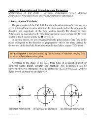
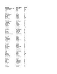
Example<br />
Compensated open loop transfer function is now<br />
Gc(s)G(s) =<br />
5(s + 0.1)<br />
(s + 1/80)<br />
1<br />
s(s + 2)<br />
Closed-loop poles of compensated system:<br />
−0.95 ± j1.98, −0.10<br />
Closed-loop poles of proportionally controlled system:<br />
−1 ± j2<br />
What do you expect from the transient response?
EE 3CL4, §6<br />
38 / 38<br />
Tim Davidson<br />
<strong>Compensator</strong>s<br />
<strong>Lead</strong><br />
compensation<br />
<strong>Design</strong> via <strong>Root</strong><br />
<strong>Locus</strong><br />
<strong>Lead</strong> <strong>Compensator</strong><br />
example<br />
Cascade<br />
compensation<br />
<strong>and</strong><br />
steady-state<br />
errors<br />
<strong>Lag</strong><br />
Compensation<br />
<strong>Design</strong> via <strong>Root</strong><br />
<strong>Locus</strong><br />
<strong>Lag</strong> compensator<br />
example<br />
Insights<br />
Insights<br />
• If we would like to improve the transient performance of<br />
a closed loop<br />
• We can try to place the dominant closed-loop poles in<br />
desired positions<br />
• One approach to doing that is lead compensator design<br />
• However, that typically requires the use of an amplifier<br />
in the compensator, <strong>and</strong> hence requires a power supply<br />
• If we would like to improve the steady-state error<br />
performance of a closed loop<br />
• We can consider designing a lag compensator to<br />
provide the required gain<br />
• However, that typically slows down the transient<br />
response<br />
• These insights also have frequency domain<br />
interpretations, which we will explore later