4.5 Geoelectrical methods - LIAG

4.5 Geoelectrical methods 

Geoelectrical methods are used extensively in 

groundwater mapping for investigation of the 

vulnerability of aquifers and shallow aquifers 

themselves. The vulnerability of aquifers is closely 

related to the heterogeneity of the clay cap. The 

clay content of the formation defines the 

electrical formation resistivity with clayish less 

permeable formations showing low resistivities 

and sandy permeable formations showing high 

resistivities. The geoelectrical method is capable 

of mapping both low and high resistive 

formations and therefore a valuable tool for 

vulnerability studies (Chistensen & Sørensen 

1998, Sørensen et al. 2005). 

The traditional single soundings in Schlumberger 

configuration or profiling in Wenner configuration 

are predominantly replaced by new 

computerized methods where profiling and 

sounding are carried out in one work process. 

The data collection is either done with multi 

electrode systems (CVES) or with an array of fixed 

electrode configurations (PACES, OhmMapper). 

In this section a brief description of the physical 

base is given. Furthermore the different 

instrument systems and field techniques, which 

have been used in the BurVal pilot areas, are 

described. Detailed descriptions of the 

geoelectrical method can be found in e.g. Binley 

& Kemna (2005), Ernstson & Kirsch (2006), and 

Ward (1990). 

4.5.1 Physical base 


A geoelectrical measurement is carried out by 

recording the electrical potential arising from 

current input into the ground with the purpose 

of achieving information on the resistivity 

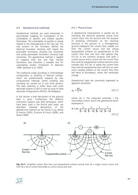
structure in the ground. In a homogeneous 

ground (halfspace) the current flow radially out 

from the current source and the arising 

equipotential surfaces run perpendicular to the 

current flow lines and form half spheres (Fig. 

4.5.1a). In the common situation with both a 

current source and a current sink the current flow 

lines and the equipotential surfaces become more 

complex (Fig. 4.5.1b). In reality the current flow 

lines and the equipotential lines will form an even 

more complex pattern as the current flow lines 

will bend at boundaries, where the resistivities 

change. 

Geoelectrical data are commonly expressed as 

apparent resistivities 

ΔV 

= K 

I 

ρ a (4.5.1) 

where ΔV is the measured potential, I the 

transmitted current, and K the geometrical factor 

expressed as 

K = 2π 

r 

A 

1 

- r 

M 

1 1 1 

- - + 

r - r r - r r - r 

A 

N 

B 

M 

B 

N 

. 

(4.5.2) 

Fig. 4.5.1: Simplified current flow lines and equipotential surfaces arising from (a) a single current source and 

from (b) a set of current electrodes (a current source and sink). 

77

78 

INGELISE MØLLER, KURT I. SØRENSEN & ESBEN AUKEN 

The apparent resistivity is defined so that it is 

equal to the true resistivity in a homogeneous 

halfspace. In Equation 4.5.2 r A and r B are positions 

of the current electrodes and r M and r N are 

positions of the potential electrodes (Fig. 4.5.1). 

Some of the most common electrode arrays are 

Wenner, Schlumberger, pole-pole, pole-dipole 

and dipole-dipole array (Fig. 4.5.2). Recently, the 

gradient array (Fig. 4.5.2) has gained renewed 

interest, since it is well suited for multichannel 

systems. Dahlin & Zhou (2004) have investigated 

the resolution capacity and efficiency of 10 

electrode arrays in a numerical modelling study. 

They find that the dipole-dipole, pole-dipole and 

the gradient arrays have the best resolution. 

However these arrays are most sensible to noise, 

whereas the often used Wenner array and the 

gamma array are less sensible to noise. Despite 

the sensibility to noise, they recommend for 2D 

resistivity surveying collected with a high data 

density, the gradient, pole-dipole and dipoledipole 

arrays as well as Schlumberger array, 

because of the resolution capacity. 

4.5.2 Field techniques 

In the following section three field techniques are 

described: the vertical electrical sounding, the 

continuous vertical electrical sounding and the 

pulled array continuous electrical sounding 

methods. 

Fig. 4.5.2: Some of the most common used electrode configurations. The letters A and B denote the current 

electrodes and the letters M and N denote the potential electrodes.

Fig. 4.5.3: Sketch of the field setup for a VES in Schlumberger configuration. 

Vertical electrical sounding 

Vertical electrical sounding, VES, is used to 

determine the resistivity variation with depth. 

Single VES should only be applied in areas, where 

the ground is assumed to be horizontal layered 

with very little lateral variation, since the 

sounding curves only can be interpreted using a 

horizontally layered earth (1D) model. A short 

description of the field technique is given here. A 

more comprehensive description can be found in, 

e.g., Ernstson & Kirsch (2006). 

A VES is typically carried out in Schlumberger 

array, where the potential electrodes are placed 

in a fixed position with a short separation and the 

current electrodes are placed symmetrically on 

the outer sides of the potential electrodes (Fig. 

4.5.3). After each resistivity measurement the 

current electrodes are moved further away from 

the centre of the array. In this way the current is 

stepwise made to flow through deeper and 

deeper parts of the ground. The positions of the 

current electrodes are typically logarithmically 

distributed with at least 10 positions per decade. 

For large distances between the current 

electrodes, the distance of the potential 

electrodes is increased to ensure that the 

measured voltage is above the noise level and the 

detection level in the instrument. 

For a VES in Schlumberger array, the distance 

between the current electrodes should be about 

250 m to detect a resistivity layer boundary in the 

depth of 50 m. 


Continuous Vertical Electrical Sounding 

Continuous vertical electrical sounding, CVES, 

combines profiling and sounding, so that a 2D 

data coverage along a profile is obtained. This 

results in an image of the resistivity structure 

along a profile. The development of the CVES 

method has taken place since the 1980’ies (e.g., 

van Overmeeren & Ritsema 1988; Dahlin 1996). 

A large number of electrodes are places on a line 

at equal distance and connected to a switching 

unit and the resistivity instrument by multicore 

cables (Fig. 4.5.4). One multicore cable has about 

20 electrode take-outs and up to three to four 

cables are used for one electrode setup. Long 

profiles are carried out using roll-along 

technique, where the last cable successively is 

moved to the front of the profile and connected 

to the first cable (Dahlin 1996). A computer, 

which typically is build into modern resistivity 

instrument, controls which electrodes are used as 

current and potential electrodes. 

Multichannel resistivity instruments become more 

and more used in stead of single channel 

resistivity meters. Data collection in Wenner 

arrays has been preferred when using single 

channel resistivity meters because of the Wenner 

arrays robustness against noise. When 

multichannel instruments are used other 

electrode arrays are more efficient. More noise 

sensible arrays are acceptable to use, when the 

data are collected with a high data density. 

Dahlin & Zhou (2004) recommend for instants 

the moving gradient array for multichannel 

instruments. 

79

80 


Fig. 4.5.4: The CVES method. a) A sketch of a field setup for CVES and data density for a profile acquired in 

Wenner configuration with 5 electrode spacings. b) Photo of the CVES system in the field. 

The productivity in the field depends on the 

density of the data points in the profiles and the 

number of channels in the resistivity instrument. 

The initial electrode spacing do also count, 

because the longer electrode spacing the longer 

distances the field crew have to walk, while they 

roll cables out, enter electrodes into the ground, 

and connect them to the cables. 

In groundwater mapping an initial electrode 

spacing of 5 m is very common. When the data 

are collected in Wenner arrays the maximum 

electrode spacing is thus typically about 100–120 

m with a total array length of 300–360 m. This 

leads to a penetration depth about 60–80 m. 

Other types of electrode arrays with similar 

maximum array lengths result in similar 

penetration depths. If the target is shallower, the 

initial electrode spacing can be decreased. This 

will also result in a higher resolution of particular 

the near surface small-scale resistivity structures. 

Pulled array continuous electrical sounding 

The PACES system was developed to meet the 

demands of high productivity, reliability and 

detailed, dense sampling (Sørensen 1996, 

Sørensen et al. 2005). Figure 4.5.5 shows 

schematics and photograph of the system. A 

small caterpillar pulls a tail of electrodes along 

with the processing electronics. The caterpillar, 

with a height of 80 cm and a width of 70 cm can 

pass under fences and in between trees. A small 

3 m platform is carried along and serves as a 

bridge for crossing small creeks and ditches. Eight 

electrode arrays are measured simultaneously 

allowing for sounding data to be acquired 

continuously along the profile (Fig. 4.5.5b). A 

crew of two workers can record profile lengths of 

10–20 km/day. 

Two electrodes with a current of 2–30 

milliamperes are maintained as sources. The 

current limit of 30 milliamperes is for the safety 

of personnel. The current is maintained at a 

constant level with a current generator in order 

to facilitate data processing. 

Processing electronics with a high input 

resistance of 5-10 Megaohms (MΩ) are mounted 

inside the potential electrodes to diminish earth 

contact problems, cross talk and capacitive 

coupling between receiver– and transmitter 

cabling in the tail. Light weighted mild-steel 

electrodes with a maximum of 10 kg are 

necessary as current and potential electrodes. 

Electrochemical interactions between the rapidly 

changing soil environment and metal potential 

electrodes are by far the largest noise sources. 

The decay time of these noise potentials is of the 

order of seconds. Clearly this is not an issue 

when using traditional metal rods, but in the case


Fig. 4.5.5: The PACES method. a) Sketch of the PACES system, where a tail of electrodes is pulled by a small 

caterpillar. b) A diagram of the eight electrode configurations, which all use the same two current electrodes. c) 

Photo of the PACES system in the field. 

of moving electrodes the influence may be 

severe. The electrochemical noise is suppressed 

by applying synchronous detection techniques 

with a frequency of 20 Hz followed by adapted 

filtering (Munkholm et al. 1995). 

Digital data acquisition is performed on-line by 

equipment on the caterpillar. The data are 

sampled with a frequency of 80 Hz and reduced 

to a dataset for every second, and the speed of 

the tail is approximately 1 m/s (3 km/h). The 

spatial averaging width in the post-processing 

stage is related to the electrode spacing and is 

usually 0.1 – 0.25 times the spacing, giving a 

detailed spatial resolution and smooth datasets. 

To monitor data quality, the system has the 

ability to detect insufficient galvanic contact at 

the current and potential electrodes while 

measuring. In addition, the magnitude of the 

emitted current is adapted automatically to 

ground contact to optimize the signal-to-noise 

ratio. The amplification in each channel adjusts 

automatically to the level of the incoming signals 

(Sørensen 1996). All parameters related to the 

measuring process are stored together with the 

data sets to insure high data quality. 

4.5.3 Data processing and inversion 

Data processing 

Geoelectrical data are normally processed by 

simply removing data influenced by noise. Figure 

4.5.6a shows an example of a data profile 

collected using gradient arrays (Dahlin & Zhou 

2004). A very simple data processing is done to 

the data and only data with a “jiggered” 

appearance are removed. The removal is done 

manual. The pseudosection in Figure 4.5.6b 

shows colour contour of the same data as in 

Figure 4.5.6a. 

Inversion 

In the following we will discuss inversion methodologies 

for CVES and PACES data focusing on the 

1-D and the 2D laterally constrained inversion 

(LCI) which uses sharp layer boundaries. 

The 1D-LCI was originally developed for inverting 

PACES data (Sørensen 1996). The data quantities 

from the PACES system are extremely large, and 

2D smooth inversion is therefore not practically 

possible on a routine basis. Because the PACES 

81

82 


Fig. 4.5.6: CVES data collected in gradient arrays are shown (a) as curves for each individual array and (b) as a 

data pseudo section. Hot colours indicate high resistivities while green and blue colours indicate low resistivities. 

system is used in sedimentary environments with 

relatively smooth lateral resistivity variations, a 

layered inversion model is desirable. 

The 1D-LCI solves a number of 1D problems 

simultaneously with constraints between 

neighbouring models (Auken et al. 2005). This 

requires that all separate 1D models have the 

same subset of model parameters. The 1D-LCI 

approach is illustrated in Figure 4.5.7. The CVES 

dataset in Figure 4.5.7a is divided into soundings 

and models. All models and corresponding 

datasets are inverted simultaneously, minimizing 

a common object function (Auken & Christiansen 

2004). The lateral constraints and constraints 

from a priori information are all part of the data 

vector together with the apparent resistivity data. 

Due to the lateral constraints, information from 

one model will spread to neighbour models. If 

the model parameters of a specific model are 

better resolved, due to, e.g., a priori information, 

this information will also spread to neighbour 

models. 

The lateral constraints can be considered as a 

priori information on the geological variability 

within the area, where the measurements are 

taken. The smaller the expected variation for a 

model parameter is, the harder the constraint. 

A priori information can be added to the dataset 

as depth to layers or layer resistivities. The 

information originates from auger– and coredrillings 

or geophysical well logs. If the a priori 

data agree with the resistivity data, the depth to 

layers in the resistivity model will coincide with


Fig. 4.5.7: a) The CVES profile is divided into n datasets. b) The datasets are inverted simultaneously with a 1D 

model resulting in a pseudo-2D image. The models are constrained laterally, and each model allows a priori 

constraints on the resistivities and thicknesses or depths. After Wisén et al. (2005). 

the a priori data. If, on the other hand, enough 

resistivity data suggest a different depth than the 

a priori data, the layer boundary in the resistivity 

model will most likely not agree with the a priori 

data. 

The 2D LCI algorithm (Auken & Christiansen 

2004) uses the same formulation of the inversion 

scheme as the 1D LCI. The difference is that the 

forward model is 2D and not 1D. This means that 

the 2D formulation can handle large lateral 

variations in the subsurface resistivity, variations 

causing the 1D formulation to output sections 

with 2D artefacts. 

A very common way of inverting CVES data is to 

use a 2D smooth inversion as presented by, e.g., 

Loke & Dahlin (2002) and Oldenburg & Li (1994). 

In the 2D smooth inversion the model is divided 

into cells and the inversion claims to some extent 

equality between neighbouring cells. The object 

function reduces a combination of data misfit 

and structure of the model to obtain a smooth 

model. This is the same as saying that the user 

picks a misfit and then the algorithm reduces 

structure of the model and data misfit to reach 

that misfit. 

Figure 4.5.8 shows the interpretation of a 300 m 

CVES profile from the southern part of Sweden. 

The resistivity survey was carried out as part of 

the geotechnical investigations for road 

construction in connection with the motorway 

connections to the Öresund bridge-tunnel 

between Denmark and Sweden. 

The data pseudo section in Figure 4.5.8a presents 

relatively smooth transitions and there are no 

clear signs of characteristic 2D structures, 

although near surface resistivity variations can be 

recognized at, e.g., profile coordinate 14.05 km. 

The minimum structure 2D inversion (Oldenburg 

& Li 1994) in Figure 4.5.8b detects a number of 

near-surface inhomogeneities along the profile. 

83

84 


Fig. 4.5.8: CVES field data. a) Data presented as a data pseudo section. b) Minimum structure 2D inversion. c) 

Stitched-together section of 1D inversion with analyses in (d). e) LCI section with analyses in (f). The colour-coding 

of the analyses ranges from well-resolved (red) to poorly resolved (blue). Two drill holes are located at 14.1 km 

and 14.2 km. The colours from the hole located at 14.2 km indicate from the bottom: grey medium fine clay 

(grey), silty sand (dark yellow), brown medium fine clay (brown) and medium sands at the top (yellow). In the drill 

hole at 14.2 km the silty layer is missing, otherwise they are the same. After Auken et al. (2005). 

Up to a depth of approximately 10 m, there 

seems to be a relatively horizontal layer with 

resistivities about 40 Ωm above a more resistive 

basement. Formation boundaries cannot be 

recognized from the inverted section. Figure 

4.5.8c presents a section of stitched-together 1D 

inversions along the profile. Indications of 

formation boundaries are seen, but they have a 

geologically unrealistic appearance mainly 

because of equivalence problems. The analyses 

(Fig. 4.5.8d) present poorly resolved parameters 

with only occasionally well determined 

parameters. The LCI model section (Fig. 4.5.8e) 

presents a model using 4 layers with smooth 

transitions in resistivities and layer boundaries, 

while still picking up the near-surface resistivity 

changes. The constraints between resistivities and 

depth interfaces used in the LCI inversion form a 

factor of 1.14. Now we can see a layered 

structure with a bowl-shape on the bottom layer 

along the profile, and we are able to differentiate 

between the two clay layers depicted in the drill 

holes. The thicknesses of the top layer and the 

brown clay layer are consistent with those found 

in the two drill holes. The silty layer is not found, 

either because it is a very local structure, as 

indicated by the drill holes, because the resistivity 

of the layer is close to that of the clay layers, or 

because the layer is too thin. The analyses (Fig. 

4.5.8f) present mainly well determined 

parameters along the profile. Only the thickness 

of the second layer is rather poorly determined 

due to the low resistivity contrast to the third 

layer. All the model sections presented produce 

data that fit the observed data to an acceptable 

level.

4.5.4 Penetration depth 

The penetration depth depends on the chosen 

electrode array, maximum electrode spacing and 

the data density. Furthermore the resistivity 

structure in the ground and the contrast of the 

resistivity structures influence on the penetration 

depth. A conductive layer close to terrain tends 

to decrease the penetration depth since the 

current primarily would flow in the conductive 

layer. If a resistive layer overlies a conductive layer 

the penetration depth may increase as the 

current tends to flow in the deeper conductive 

layer. 

In an area with glacial deposits like in Denmark, 

northern Germany and parts of The Netherlands 

the geological variability is relatively large, thus it 

is very helpful to introduce the term “robust 

penetration depth”. When you talk about robust 

penetration depth the dimension in the data is 

taken into account. A CVES dataset is collected 

along a profile and interpreted using a 2D 

resistivity model, though the geological setting 

and the thereby resistivity structure varies in three 

dimensions. At large electrode spacings in a CVES 

profile the volume of the ground also 

perpendicular to the array and profile direction 

becomes so large that resistivity variations also 

perpendicular to the profile start to influence in 

the measurements. In Denmark the experience is 

that for a CVES profile the robust penetration 

depth is about 60 m. Likewise a VES maps the 

resistivity variation with depth at one point and is 

interpreted using a 1D resistivity model thus the 

resistivity structure may vary in three dimensions. 

For a VES it is even more critical if there are 

resistivity variations in the direction of the 

electrode array. 

4.5.5 Resolution 

It is difficult to give quantitative measures for the 

resolution. It depends on the number and the 

type of electrode arrays used, the resistivity 

structures and the resistivity contrast of the 

resistivity structures. Numerical studies for 1D 

models can be carried out in a systematic way 

(e.g., Christensen & Sørensen 2001). There are 

only a few examples on studies of the resolution 

of 2D models. Dahlin & Zhou (2004) show how 

different electrode arrays resolve five different 2D 


models. From these results it is clearly seen that 

the resolution decreases both vertically and 

laterally by depth. 

By a rule of thump a horizontal resistivity 

structure should have a thickness of about 1.5–2 

times the layers above it to be well determined in 

a resistivity model. Thinner resistivity structures 

may be seen in the data and indication of the 

structure will appear in the resistivity model. 

Resistivity structures thinner than 1.5–2 times the 

layers above it may suffer from equivalences (see 

Sect. 4.5.6.). 

4.5.6 Restrictions, uncertainties, error 

sources and pitfalls 

Restrictions in penetration depth with lowvoltage 

equipment 

The small low-voltage resistivity meters, which 

usually are used in groundwater surveys, would 

normally be applicable for mapping in the upper 

100 m. If deeper penetration is wanted, very 

large electrode spacings must be used, which 

require high voltage for generating enough 

current to arise a detectable potential difference. 

This means that heavier equipment including 

strong generators is needed for the fieldwork. In 

the planning of a geoelectrical survey with deep 

penetration depth, it is important to judge if the 

geological setting is suited for 1D or 2D data 

collection (see Sect. 4.5.4 Penetration depth). 

Principle of equivalence 

The “principle of equivalence” is a serious 

problem for geoelectrical data. Equivalences 

occur, where a resistive layer lies in between two 

conductive layers or vice versa. If a relatively thin 

resistive layer lies in between two conductive 

layers, it may only be possible to determine the 

resistance of the layer, i.e., the product of the 

resistivity and the thickness. Therefore, a resistive 

layer and a layer with the half thickness and the 

double resistivity give very equal responses. 

Resistive layers should have a thickness more 

than 1.5–2 times the layers above it before the 

resistivity and the thickness of the layer can be 

resolved independently. 

85

86 


In the opposite case, where a conductive layer 

lies in between two resistive layers, it may only be 

possible to determine the conductance of the 

layer, i.e., the thickness divided by the resistivity. 

Therefore a conductive layer and a layer with the 

double resistivity and double thickness give very 

equal responses. The conductive layer also has to 

be about 1.5–2 times as thick as the layers in 

total above it to be determined by both its 

thickness and resistivity separately. 

In the interpretation of geoelectrical data it is 

important to take the possibility of equivalence 

into account since equivalent models may lead to 

quite different hydrogeological models. If we 

have a sand and gravel layer of high resistivity in 

between two clay layer of low resistivity that 

suffers from equivalence, the high resistive layer 

may either be interpreted as a thin layer of 

unsaturated sand and gravel or the thicker layer 

of saturated sand and gravel. 

Electromagnetic noise and other cultural 

noise sources 

Geoelectrical measurements are in general robust 

towards electromagnetic noise. Although one 

should avoid locating profiles parallel to highvoltage 

power lines. A safety distance of about 

1.5 to 2 times the expected penetration depth 

should ensure a good data quality. 

Elongated resistivity anomalies that are parallel to 

2D resistivity profiles may distort the data. If a 2D 

resistivity profile is placed parallel to an elongated 

good conductor like a metallic fence with 

galvanic contact to the ground, buried metal 

pipes or cables with a metallic casing, current can 

be channelled through the good conductor. It 

should also be avoided to place the profiles 

parallel to other elongated resistivity anomalies 

like road beds, dykes, ditches and streams 

because the symmetry of the current density 

parallel to the profile is distorted. A safety 

distance of about 1.5 to 2 times the expected 

penetration depth should also here ensure a 

good data quality. 

2D resistivity profiles that cross cultural resistivity 

anomalies perpendicular cause no problem. A 

thin metal pipe may even not cover a large 

enough area to be detected. 

Season of field work 

The best and less noisy data are collected if a 

good contact to the ground is present. A good 

ground contact results in a relative low contact 

resistance between the electrodes and the 

ground, which ensure that relative high current 

can be suppressed into the ground. Good contact 

between the electrodes and the ground is 

obtained, when the soil is moist and at least 

partly saturated by water. It can be difficult to 

obtain a good data quality or even to collect 

data, if the soil at ground surface is completely 

dry. In an area with dry soil, the data quality can 

be enhanced, if the soil around the electrodes are 

watered by salty water, thus it is labour-intensive. 

In agricultural areas the field work may be 

restricted to seasons of the year, where no crop is 

in the field or the plants still are small. 

4.5.7 References 

Auken E, Christiansen AV (2004): Layered and 

laterally constrained 2D inversion of resistivity 

data. – Geophysics 69: 752–761. 

Auken E, Christiansen AV, Jacobsen BH, Foged N, 

and Sørensen KI (2005): Piecewise 1D 

Laterally Constrained Inversion of resistivity 

data. – Geophysical Prospecting 53: 497–506. 

Binley A, Kemna A (2005): DC resistivity and 

induced polarization methods. – In Yuram R, 

Hubbard SS (eds.): Hydrogeophysics. Water 

and Science Technology Library 50: 129–156. 

Springer, New York. 

Christensen NB, Sørensen KI (1998): Surface and 

borehole electric and electromagnetic 

methods for hydrogeological investigations. – 

European Journal of Environmental and 

Engineering Geophysics 3: 75–90. 

Christensen NB, Sørensen K (2001): Pulled array 

continuous electrical sounding with an 

additional inductive source: an experimental 

design study. – Geophysical Prospecting 49: 

241–254. 

Dahlin T (1996): 2D resistivity surveying for 

environmental and engineering applications. – 

First Break 14: 275–283.

Dahlin T, Zhou B (2004): A numerical comparison 

of 2D resistivity imaging with 10 electrode 

arrays. – Geophysical Prospecting 52: 379– 

398. 

Ernstson K, Kirsch R (2006): Geoelectrical 

methods, basic principles. – In Kirsch R (ed): 

Groundwater Geophysics: A Tool for 

Hydrology, 85–108. Springer. 

Loke MH, Dahlin T (2002): A comparison of the 

Gauss-Newton and quasi-Newton methods in 

resistivity imaging inversion. – Journal of 

Applied Geophysics 49: 149–162. 

Munkholm MS, Sørensen KI, Jacobsen BH (1995): 

Characterization and in-field suppression of 

noise in Hydrogeophysics. – In: Proceedings of 

the Symposium on the Application of 

Geophysics to Engineering and Environmental 

Problems (SAGEEP), Orlando, Florida: 339– 

348. 

Oldenburg DW, Li Y (1994): Inversion of induced 

polarization data. – Geophysics 59: 1327– 

1341. 


Sørensen KI, Auken E, Christensen NB, Pellerin L 

(2005): An Integrated Approach for 

Hydrogeophysical Investigations: New 

Technologies and a Case History. – In Butler D 

K (ed.) Near-Surface Geophysics 2, 

Investigations in Geophysics 13: 585–603. 

Society of Exploration Geophysics. 

Sørensen KI (1996): Pulled Array Continuous 

Electrical Profiling. – First Break 14: 85–90. 

van Overmeeren RA, Ritsema IL (1988): 

Continouos vertical electrical sounding. – First 

Break 6: 313–324. 

Ward SH (1990): Resistivity and induced 

polarization methods. – In Ward SH (ed.): 

Geotechnical and Environmental Geophysics 

1, Investigations in Geophysics 5: 147–189. 

Society of Exploration Geophysics. 

Wisén R, Auken E, Dahlin T (2005): Combination 

of 1D laterally constrained inversion and 2D 

smooth inversion of resistivity data with a 

priori data from boreholes. – Near Surface 

Geophysics 3: 71–79. 

87

88 

INGELISE MØLLER, KURT I. SØRENSEN & ESBEN AUKEN

4.5 Geoelectrical methods - LIAG

You also want an ePaper? Increase the reach of your titles

Delete template?

Save as template?