4.5 Geoelectrical methods - LIAG

84
INGELISE MØLLER, KURT I. SØRENSEN & ESBEN AUKEN
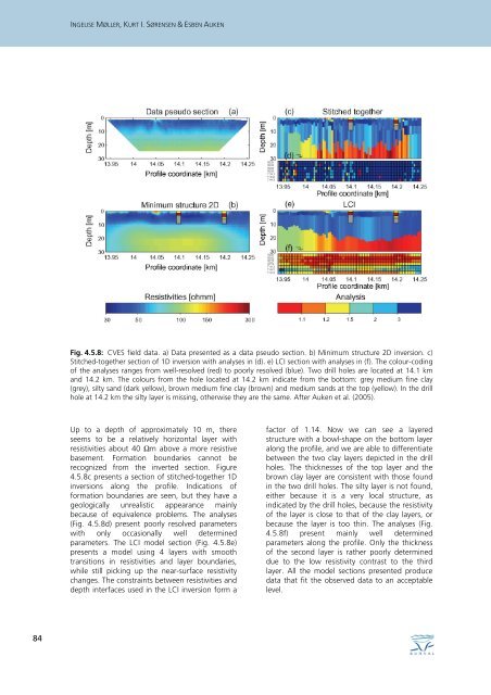
Fig. 4.5.8: CVES field data. a) Data presented as a data pseudo section. b) Minimum structure 2D inversion. c)
Stitched-together section of 1D inversion with analyses in (d). e) LCI section with analyses in (f). The colour-coding
of the analyses ranges from well-resolved (red) to poorly resolved (blue). Two drill holes are located at 14.1 km
and 14.2 km. The colours from the hole located at 14.2 km indicate from the bottom: grey medium fine clay
(grey), silty sand (dark yellow), brown medium fine clay (brown) and medium sands at the top (yellow). In the drill
hole at 14.2 km the silty layer is missing, otherwise they are the same. After Auken et al. (2005).
Up to a depth of approximately 10 m, there
seems to be a relatively horizontal layer with
resistivities about 40 Ωm above a more resistive
basement. Formation boundaries cannot be
recognized from the inverted section. Figure
4.5.8c presents a section of stitched-together 1D
inversions along the profile. Indications of
formation boundaries are seen, but they have a
geologically unrealistic appearance mainly
because of equivalence problems. The analyses
(Fig. 4.5.8d) present poorly resolved parameters
with only occasionally well determined
parameters. The LCI model section (Fig. 4.5.8e)
presents a model using 4 layers with smooth
transitions in resistivities and layer boundaries,
while still picking up the near-surface resistivity
changes. The constraints between resistivities and
depth interfaces used in the LCI inversion form a
factor of 1.14. Now we can see a layered
structure with a bowl-shape on the bottom layer
along the profile, and we are able to differentiate
between the two clay layers depicted in the drill
holes. The thicknesses of the top layer and the
brown clay layer are consistent with those found
in the two drill holes. The silty layer is not found,
either because it is a very local structure, as
indicated by the drill holes, because the resistivity
of the layer is close to that of the clay layers, or
because the layer is too thin. The analyses (Fig.
4.5.8f) present mainly well determined
parameters along the profile. Only the thickness
of the second layer is rather poorly determined
due to the low resistivity contrast to the third
layer. All the model sections presented produce
data that fit the observed data to an acceptable
level.