4.5 Geoelectrical methods - LIAG

More documents

Recommendations

Info

82 INGELISE MØLLER, KURT I. SØRENSEN & ESBEN AUKEN Fig. 4.5.6: CVES data collected in gradient arrays are shown (a) as curves for each individual array and (b) as a data pseudo section. Hot colours indicate high resistivities while green and blue colours indicate low resistivities. system is used in sedimentary environments with relatively smooth lateral resistivity variations, a layered inversion model is desirable. The 1D-LCI solves a number of 1D problems simultaneously with constraints between neighbouring models (Auken et al. 2005). This requires that all separate 1D models have the same subset of model parameters. The 1D-LCI approach is illustrated in Figure 4.5.7. The CVES dataset in Figure 4.5.7a is divided into soundings and models. All models and corresponding datasets are inverted simultaneously, minimizing a common object function (Auken & Christiansen 2004). The lateral constraints and constraints from a priori information are all part of the data vector together with the apparent resistivity data. Due to the lateral constraints, information from one model will spread to neighbour models. If the model parameters of a specific model are better resolved, due to, e.g., a priori information, this information will also spread to neighbour models. The lateral constraints can be considered as a priori information on the geological variability within the area, where the measurements are taken. The smaller the expected variation for a model parameter is, the harder the constraint. A priori information can be added to the dataset as depth to layers or layer resistivities. The information originates from auger– and coredrillings or geophysical well logs. If the a priori data agree with the resistivity data, the depth to layers in the resistivity model will coincide with
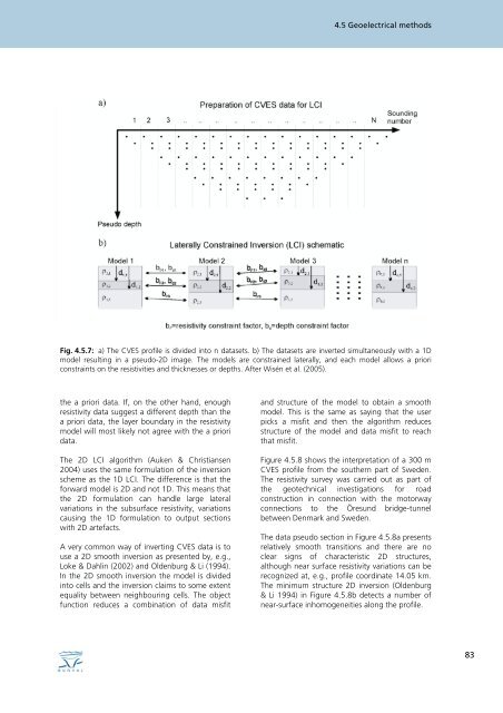
4.5 Geoelectrical methods Fig. 4.5.7: a) The CVES profile is divided into n datasets. b) The datasets are inverted simultaneously with a 1D model resulting in a pseudo-2D image. The models are constrained laterally, and each model allows a priori constraints on the resistivities and thicknesses or depths. After Wisén et al. (2005). the a priori data. If, on the other hand, enough resistivity data suggest a different depth than the a priori data, the layer boundary in the resistivity model will most likely not agree with the a priori data. The 2D LCI algorithm (Auken & Christiansen 2004) uses the same formulation of the inversion scheme as the 1D LCI. The difference is that the forward model is 2D and not 1D. This means that the 2D formulation can handle large lateral variations in the subsurface resistivity, variations causing the 1D formulation to output sections with 2D artefacts. A very common way of inverting CVES data is to use a 2D smooth inversion as presented by, e.g., Loke & Dahlin (2002) and Oldenburg & Li (1994). In the 2D smooth inversion the model is divided into cells and the inversion claims to some extent equality between neighbouring cells. The object function reduces a combination of data misfit and structure of the model to obtain a smooth model. This is the same as saying that the user picks a misfit and then the algorithm reduces structure of the model and data misfit to reach that misfit. Figure 4.5.8 shows the interpretation of a 300 m CVES profile from the southern part of Sweden. The resistivity survey was carried out as part of the geotechnical investigations for road construction in connection with the motorway connections to the Öresund bridge-tunnel between Denmark and Sweden. The data pseudo section in Figure 4.5.8a presents relatively smooth transitions and there are no clear signs of characteristic 2D structures, although near surface resistivity variations can be recognized at, e.g., profile coordinate 14.05 km. The minimum structure 2D inversion (Oldenburg & Li 1994) in Figure 4.5.8b detects a number of near-surface inhomogeneities along the profile. 83
Page 1 and 2: 4.5 Geoelectrical methods Geoelectr
Page 3 and 4: Fig. 4.5.3: Sketch of the field set
Page 5: 4.5 Geoelectrical methods Fig. 4.5.
Page 9 and 10: 4.5.4 Penetration depth The penetra
Page 11 and 12: Dahlin T, Zhou B (2004): A numerica

4.5 Geoelectrical methods - LIAG

You also want an ePaper? Increase the reach of your titles

Delete template?

Save as template?