Discontinuous Galerkin methods Lecture 3 - Brown University

Let us also consider a slightly more complicated problem, originating
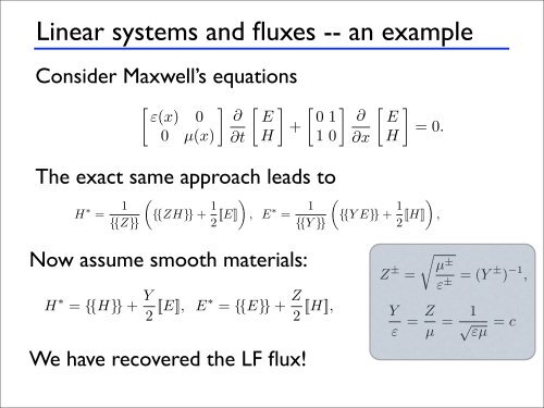
Linear systems and fluxes -- an example
electromagnetics.
2.5 Exercises 39
Example Consider 2.6. Consider Maxwell’s the equations
one-dimensional Maxwell’s equations
1
ε(x) 0 ∂ E 01 ∂ E
{{ZH}} + +
=0. (2.2
{{Z}}
0 µ(x) ∂t H 10 ∂x H
1
2 [[E]]
, E ∗ = 1
{{YE}} +
{{Y }}
1
2 [[H]]
or
H
,
∗ = 1
{{ZH}} +
{{Z}}
1
2 [[E]]
, E ∗ = 1
{{Y }}
where
Z ±
µ ±
=
ε ± =(Y ± ) −1 ,
2.5 Exercises 39
Here (E, H) = (E(x, t),H(x, t)) represent the electric and magnetic fiel
respectively, while ε and µ are the electric and magnetic material propertie
known as permittivity and permeability, respectively.
To simplify the notation, let us write this as
Q ∂q
+ A∂q
∂t ∂x =0,
or
H
where
ε(x) 0
01 E
Q =
, A = , q = ,
0 µ(x) 10 H
reflect the spatially varying material coefficients, the one-dimensional rotatio
operator, and the vector of state variables, respectively.
∗ = 1
{{ZH}} +
{{Z}}
1
2 [[E]]
, E ∗ = 1
{{YE}} +
{{Y }}
1
2 [[H]]
,
where
Z ±
µ ±
=
ε ± =(Y ± ) −1 ,
represents the impedance of the medium.
If we again consider the simplest case of a continuous medium, things
simplify considerably as
H ∗ = {{H}} + Y
2 [[E]], E∗ = {{E}} + Z
2 [[H]],
or
H
which we recognize as the Lax-Friedrichs flux since
∗ = 1
{{ZH}} +
{{Z}}
1
2 [[E]]
, E ∗ = 1
{{Y }}
where
Z ±
µ ±
=
ε ± =(Y ± ) −1 ,
represents the impedance of the medium.
If we again consider the simplest case of a cont
simplify considerably as
H ∗ = {{H}} + Y
2 [[E]], E∗ Z
= {{E}} +
±
µ ±
=
ε ± =(Y ± ) −1 ,
the impedance of the medium.
again consider the simplest case of a continuous medium, things
onsiderably as
H ∗ = {{H}} + Y
2 [[E]], E∗ = {{E}} + Z
2 [[H]],
recognize as the Lax-Friedrichs flux since
Y Z
=
ε µ = 1
represents the impedance of the medium.
If we again consider the simplest case of a cont
simplify considerably as
H
√ = c
εµ ∗ = {{H}} + Y
2 [[E]], E∗ = {{E}} +
which we recognize as the Lax-Friedrichs flux since
Y Z
=
ε µ = 1
The exact same approach leads to
Now assume smooth materials:
√ = c
εµ
We have recovered isthe the LF speed flux!
of light (i.e., the fastest wave speed in th
−1 −1/2