Discontinuous Galerkin methods Lecture 3 - Brown University

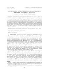
determinant continues to increase in size with N, reflecting a well-behaved
interpolation where ℓi(r) takes small values in between the nodes. For the
Local approximation - an example
equidistant nodes, the situation is entirely different.
While the determinant has comparable values for small values of N, the
determinant for the equidistant nodes begins to decay exponentially fast once
N exceeds So does 16, caused it really by the matter? close to linear -- dependence consider of Vthe
last columns
a)
c)
1.00 −1.00 1.00 −1.00 1.00 −1.00 1.00
1.00 −0.67 0.44 −0.30 0.20 −0.13 0.09
1.00 −0.33 0.11 −0.04 0.01 −0.00 0.00
1.00 0.00 0.00 0.00 0.00 0.00 0.00
1.00 0.33 0.11 0.04 0.01 0.00 0.00
1.00 0.67 0.44 0.30 0.20 0.13 0.09
1.00 1.00 1.00 1.00 1.00 1.00 1.00
0.71 −1.22 1.58 −1.87 2.12 −2.35 2.55
0.71 −0.82 0.26 0.49 −0.91 0.72 −0.04
0.71 −0.41 −0.53 0.76 0.03 −0.78 0.49
0.71 0.00 −0.79 0.00 0.80 0.00 −0.80
0.71 0.41 −0.53 −0.76 0.03 0.78 0.49
0.71 0.82 0.26 −0.49 −0.91 −0.72 −0.04
0.71 1.22 1.58 1.87 2.12 2.35 2.55
b)
d)
1.00 −1.00 1.00 −1.00 1.00 −1.00 1.00
1.00 −0.83 0.69 −0.57 0.48 −0.39 0.33
1.00 −0.47 0.22 −0.10 0.05 −0.02 0.01
1.00 0.00 0.00 0.00 0.00 0.00 0.00
1.00 0.47 0.22 0.10 0.05 0.02 0.01
1.00 0.83 0.69 0.57 0.48 0.39 0.33
1.00 1.00 1.00 1.00 1.00 1.00 1.00
0.71 −1.22 1.58 −1.87 2.12 −2.35 2.55
0.71 −1.02 0.84 −0.35 −0.28 0.81 −1.06
0.71 −0.57 −0.27 0.83 −0.50 −0.37 0.85
0.71 0.00 −0.79 0.00 0.80 0.00 −0.80
0.71 0.57 −0.27 −0.83 −0.50 0.37 0.85
0.71 1.02 0.84 0.35 −0.29 −0.81 −1.06
0.71 1.22 1.58 1.87 2.12 2.35 2.55
Bad points Good points
Fig. 3.1. Entries of V for N = 6 and different choices of the basis, ψn(r), and
evaluation points, ξi. For (a) and (c) we use equidistant points and (b) and (d) are
based on LGL points. Furthermore, (a) and (b) are based on V computed using a
simple monomial basis, ψn(r) =r n−1 , while (c) and (d) are based on the orthonormal
Bad
basis
Good
basis