Discontinuous Galerkin methods Lecture 3 - Brown University

Lagrange polynomial, ℓ
Approximation theory
k i (x). The connection between these two forms is through
the expansion coefficients, ûk n. We return to a discussion of these choices in much m
for now it suffices to assume that we have chosen one of these representations.
The global solution u(x, t) is then assumed to be approximated by the piecew
polynomial approximation uh(x, t),
K
u(x, t) uh(x, t) = u
k=1
k K
, v) Ω,h = (u, v) k
D , u
k=1
h(x, t),
2 Ω,h =(u, u) Ω,h .
cts that Ω is only approximated by the union of D k , that is
K
Ω Ωh = D
k=1
k K
u(x, t) uh(x, t) = u
k=1
Recall
,
not distinguish we assume the twothe domains local unless solution needed. to be
has local information as well as information from the neighong
an intersection between two elements. Often we will refer
ese intersections in an element as the trace of the element.
e discuss here, we will have two or more solutions or boundthe
same physical location along the trace of the element.
k h(x k ,t).
The careful reader will note that this notation is a bit careless, as we do not
address what exactly happens at the overlapping interfaces. However, a more
careful definition does not add anything essential at this point and we will use
this notation to reflect that the global solution is obtained by combining the
K local solutions as defined by the scheme.
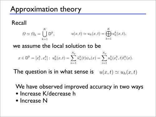
The local solutions are assumed to be of the form
x ∈ D k =[x k l ,x k r]: u k Np
h(x, t) = û
n=1
k Np
n(t)ψn(x) = u
i=1
k h(x k i ,t)ℓ k Here, we have introduced two complementary expressions
known as the modal form, we use a local polynomial basis
be ψn(x) =x
i (x).
n−1 . In the alternative form, known as the n
N + 1 local grid points, xk i ∈ Dk , and express the polynom
Lagrange polynomial, ℓk i (x). The connection between thes
the expansion coefficients, ûk n. We return to a discussion of
for now it suffices to assume that we have chosen one of th
The global solution u(x, t) is then assumed to be app
polynomial approximation uh(x, t),
K
The question is in what sense is
u(x, t) uh(x, t) =
We have observed improved accuracy in two ways
• Increase K/decrease h
• Increase N
k=1
u