Discontinuous Galerkin methods Lecture 3 - Brown University

know that
with λ > 0; that is, the wave corresponding to λ1 is entering the domain, the
λ1 = −λ, λ2 =0, λ3 = λ,
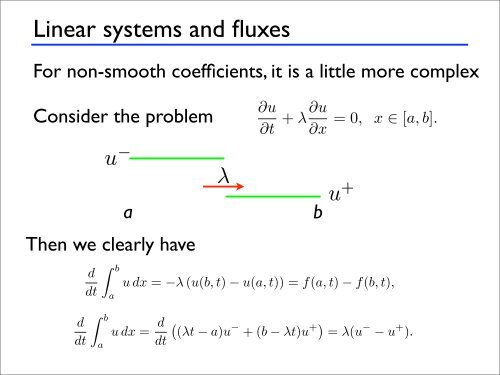
Linear systems and fluxes
∀i : −λiQ[u − − u + ] + [(Πu) − − (Πu) + ]=0
wave corresponding to λ3 is leaving, and λ2 corresponds to a stationary wave
must hold across each wave. This is also known as the Ra
condition and is a simple consequence of conservation of u ac
discontinuity. To appreciate this, consider the scalar wave eq
∂u
Consider the problem + λ∂u =0, x ∈ [a, b].
∂t ∂x
Integrating u over the interval, we have
−
with λ > 0; that is, the wave corresponding to λ1 is entering the domain, the
wave corresponding to λ3 is leaving, and λ2 corresponds to a stationary wave
as illustrated in Fig. 2.3.
Following the well-developed theory or Riemann solvers [218, 303], we
know that
∀i : −λiQ[u
λ
− − u + ] + [(Πu) − − (Πu) + as illustrated in Fig. 2.3.
Following the well-developed theory or Riemann solvers [218, 303], we
know that
∀i : −λiQ[u
]=0, (2.20)
must hold across each wave. This is also known as the Rankine-Hugoniot
condition and is a simple consequence of conservation of u across the point of
discontinuity. To appreciate this, consider the scalar wave equation
− − u + ] + [(Πu) − − (Πu) + ]=0, (2.20)
must hold across each wave. This is also known as the Rankine-Hugoniot
condition and is a simple consequence of conservation of u across the point of
discontinuity. To appreciate this, consider the scalar wave equation
∂u
+ λ∂u =0, x ∈ [a, b].
∂t ∂x
For non-smooth coefficients, it is a little more complex
d
dt
Then we clearly have
b
Integrating over the interval, ∂u we have
∂t a
∂x
b
d
Integrating over the interval, we have
u dx = −λ (u(b, t) − u(a, t)) = f(a, t) − f(b
a + λ∂u =0, x ∈ [a, b]. b
since f u= dx λu. = −λ On(u(b, thet) other − u(a, hand, t)) = f(a, since t) −the f(b, wave t), is propagati
dt a
speed, λ, we also have
b
d
dt
u dx = d
dt
u +
since f = λu. d On the u dx other = −λ hand,
dt (u(b, t) since − u(a, thet)) wave = f(a, is propagating t) − f(b, t), at a constant
speed, λ, we also b
a have
b
(λt − a)u − +(b − λt)u + = λ(u −
since f = λu. d On the other ahand,
since the wave is propagating at a constant
speed, λ, we alsou dt
have dx = d − +
(λt − a)u +(b− λt)u
dt
= λ(u − − u + ).
Taking a → x− and b → x + a
, we recover the jump conditions
d b
d − + Taking a → x − +
− and b → x + , we recover the jump conditions