Fourier Series and Partial Differential Equations Lecture Notes

Chapter 5. Laplace’s equation in the plane 54
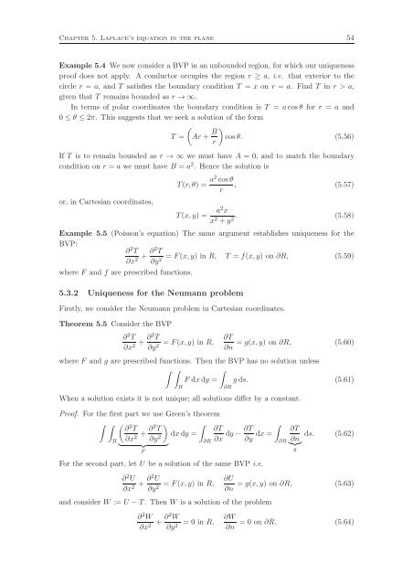
Example 5.4 We now consider a BVP in an unbounded region, for which our uniqueness
proof does not apply. A conductor occupies the region r ≥ a, i.e. that exterior to the
circle r = a, and T satisfies the boundary condition T = x on r = a. Find T in r > a,
given that T remains bounded as r → ∞.
In terms of polar coordinates the boundary condition is T = acosθ for r = a and
0 ≤ θ ≤ 2π. This suggests that we seek a solution of the form
T = Ar + B
cosθ. (5.56)
r
If T is to remain bounded as r → ∞ we must have A = 0, and to match the boundary
condition on r = a we must have B = a 2 . Hence the solution is
or, in Cartesian coordinates,
T(r,θ) = a2cosθ , (5.57)
r
T(x,y) = a2 x
x 2 +y 2.
(5.58)
Example 5.5 (Poisson’s equation) The same argument establishes uniqueness for the
BVP:
∂2T ∂x2 + ∂2T = F(x,y) in R, T = f(x,y) on ∂R,
∂y2 (5.59)
where F and f are prescribed functions.
5.3.2 Uniqueness for the Neumann problem
Firstly, we consider the Neumann problem in Cartesian coordinates.
Theorem 5.5 Consider the BVP
∂2T ∂x2 + ∂2T = F(x,y) in R,
∂y2 ∂T
∂n
= g(x,y) on ∂R, (5.60)
where F and g are prescribed functions. Then the BVP has no solution unless
F dxdy = gds. (5.61)
R
When a solution exists it is not unique; all solutions differ by a constant.
Proof. For the first part we use Green’s theorem
∂2T R ∂x2 + ∂2T ∂y2
∂T ∂T
dxdy = dy −
∂R ∂x ∂y
F
For the second part, let U be a solution of the same BVP i.e.
∂2U ∂x2 + ∂2U = F(x,y) in R,
∂y2 ∂R
∂U
∂n
dx =
and consider W := U −T. Then W is a solution of the problem
∂2W ∂x2 + ∂2W = 0 in R,
∂y2 ∂W
∂n
∂R
∂T
∂n
g
ds. (5.62)
= g(x,y) on ∂R, (5.63)
= 0 on ∂R. (5.64)