Selecting the Appropriate Numerical Soft - Polymath Software

Selecting the Appropriate Numerical Software
for a Chemical Engineering Course
Mordechai Shacham, shacham@bgumail.bgu.ac.il
Chemical Engineering Department, Ben-Gurion University of the Negev, Beer-Sheva 84105, Israel
Michael B. Cutlip, mcutlip@uconnvm.uconn.edu
Chemical Engineering Department, University of Connecticut, Storrs, CT 06269, USA
Abstract
Criteria for evaluating mathematical software packages and the results of a recent comparison of such packages are
briefly reviewed. A benchmark problem that was developed based on the results of this comparison is presented.
This problem can be used in various courses, representing various levels of knowledge in chemical process analysis,
mathematical modeling and numerical methods where the solution is achieved using the software most appropriate
to the objectives of the particular course. This work demonstrates and illustrates the conclusion that the most educational
benefits can be gained by using several packages throughout the chemical engineering curriculum. The software
that is most appropriate for a particular course must be determined according to the course objectives and the
previous exposure of the students to mathematical models, numerical algorithms and computer programming.
Keywords. Mathematical software, Numerical methods, Modeling, Chemical engineering, Problem solving
INTRODUCTION
Numerical software is routinely and extensively used
for problem solving in recent years in some of the
core chemical engineering courses ( the “process dynamics
and control” and “chemical reaction engineering”
courses, for example), but in many of the
courses the use of computers is still disappointingly
low. This may contribute to the finding that the number
of practicing engineers who use numerical software
for process design is below 10% as was found
in a recent survey (Davis et al., 1994).
This underutilization of computers and numerical
solution packages in some of the ChE courses has
been attributed to the following (Shacham et al.,
1996): The examples and homework problems given
in many of the textbooks are retained from the precomputer
era, and thus they can be solved either with
or without a computer. These problems do not encourage
educators and students to use numerical
software. Furthermore, most departments typically
select one numerical computation package to be used
by their students, and this package may be inappropriate
for use in a particular course. It may even be
too difficult to be used by the less computer-literate
students.
The departmental computer expert typically does the
identification of a package for general departmental
use. Often this expert will select the package that is
the most powerful, most flexible, and gives the user
the widest range of options. Typically some research
usage has been given strong emphasis. However,
other attributes of the package may be more important
for educational use by undergraduates. The
package must have enough capabilities to solve most
problems encountered in a particular course and it
should serve properly the objective of the course.
Serving the objective of the course means that the
effort spent in learning to use and using the package
for achieving the course objectives should be minimized.
This requirement puts more emphasis on user
friendliness and shorter learning curve than on the
power and the options provided by the software.
Cutlip and Shacham (1999) have published recently a
book entitled Problem Solving in Chemical Engineering
with Numerical Methods that contains examples
and homework assignments that require the use
of computer for their solution for most required
chemical engineering courses. The examples and
assignments in this book demonstrate for the students
and instructors the benefits of the use of the software
packages in solving realistic engineering problems.
Criteria for comparing mathematical software for
educational use has been developed (Shacham et al.,
1998, Shacham and Cutlip, 1998). Ten representative
problems from various required Chemical Engineering
courses were selected and this set of problems
was solved using six numerical software packages
including Excel, MAPLE, MATHCAD, MATLAB,
MATHEMATICA, and POLYMATH. Details of
some comparisons are given by Shacham and Cutlip,
1998.
The main conclusion from this comparison was that
there is no single package which is the best for all the
courses, but the most appropriate package must be
selected according to the objectives of the course and
the students previous exposure to mathematical models,
numerical algorithms and computer programming.
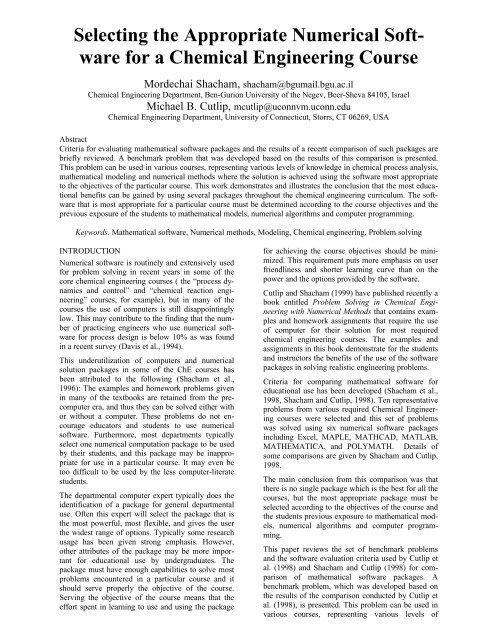
This paper reviews the set of benchmark problems
and the software evaluation criteria used by Cutlip et
al. (1998) and Shacham and Cutlip (1998) for comparison
of mathematical software packages. A
benchmark problem, which was developed based on
the results of the comparison conducted by Cutlip et
al. (1998), is presented. This problem can be used in
various courses, representing various levels of

knowledge in chemical process analysis, mathematical
modeling and numerical methods where the solution
is achieved using the most appropriate software
so as to attain the objectives of the particular course.
A BENCHMARK PROBLEM SET FOR
SOFTWARE PACKAGE EVALUATION
The set of benchmark problems of Cutlip et al.
(1998), which was developed for evaluation of software
packages, is shown in Table 1. Within this set
there are representative problems from almost every
required course in a typical chemical engineering
curriculum. This problem set has been solved with
six software packages. The CACHE Corporation
provides this problem set as well as the individual
package write-ups and problem solutions files for
downloading from the Internet at
http://www.che.utexas.edu/cache/.
Table 1 – Benchmark Problem Set
Problem Title
1 Molar Volume and Compressibility Factor
from Van Der Waal’s Equation
2 Steady State Material Balances on a Separation
Train
3 Vapor Pressure Data Representation by Polynomials
and Equations
4 Reaction Equilibrium for Multiple Gas Phase
Reactions
5 Terminal Velocity of Falling Particles
6 Unsteady State Heat Exchange in a Series of
Agitated Tanks
7 Diffusion with Chemical Reaction in a One
Dimensional Slab
8 Binary Batch Distillation
9 Reversible, Exothermic, Gas Phase Reaction in
a Catalytic Reactor
10 Dynamics of a Heated Tank with PI Temperature
Control
CRITERIA FOR SOFTWARE EVALUATION
Shacham et al. (1998) and Shacham and Cutlip
(1998) have suggested the following criteria for software
evaluation and comparison:
1. Numerical Performance
1.1. Ability to solve all typical benchmark
problems
2. User Friendliness
2.1. Menu versus command based program
control
2.2. Notation and format used in equation entry
2.3. Debugging aids (syntax errors, undefined
or not initialized variables, etc.)
2.4. Equation ordering and detection of implicit
relationships
2.5. Solution verification
3. Technical effort required for:
3.1. Preparation of the model
3.2. Documentation of the model
3.3. Setting up the solution algorithm
3.4. Presentation of the results
2
3.5. Documentation of the results
3.6. Alteration of the model for parametric
studies
Most of the above criteria are self-explanatory. More
detailed discussions of the various criteria are provided
in the references.
SELECTING THE APPROPRIATE SOFTWARE
BASED ON COURSE OBJECTIVES
Our work and experience with mathematical software,
as well as the results of the comparison that
was described in the previous sections, has lead us to
conclude that the most educational benefit can be
gained by using several packages throughout the curriculum.
The software that is most appropriate for a
particular course must be determined according to the
course objectives and the students previous exposure
to mathematical models, numerical algorithms and
computer programming. The software selection procedure
will be demonstrated in reference to a homework
assignment that is outlined below. The complete
paper including the problem statement and detailed
solutions are available on the Internet at
http://www.polymath-software.com/papers/.
RIGOROUS DISTILLATION CALCULATIONS BY THE
WANG AND HENKE METHOD - PROBLEM DEFINITION
Numerical Methods. Solution of a single nonlinear algebraic
equation, solution of systems of linear algebraic
equations.
Concepts used. Calculation of bubble point temperature for
a multicomponent mixture. Material and energy balance on
an equilibrium stage. Use of the Wang and Henke method
for rigorous distillation calculation.
Course (and Software) Usage. (I) Basic Principles and
Calculations (Excel, POLYMATH), (II) Separation Processes
(Excel, POLYMATH, HYSIS), (III) Process Modeling
and Simulation (Matlab, HYSIS)
Problem Statement. A simple distillation column with three
theoretical stages is used to separate n-hexane (1) and noctane
(2). Feed with flow rate of F (kgmol/hr) and composition
of z 1 and z 2 (mole fractions) enters the column at its
bubble point on tray No. 2. The column’s operating pressure
is P (mmHg). A total condenser is used and the
amount of heat added to the reboiler is Q (kcal/hr). Distillate
is removed at the rate of D (kgmol/hr).
The vapor-liquid equilibrium ratios (k j) can be calculated
assuming ideal solutions, thus k j = P j/P, where P j is the
vapor pressure of component j. The vapor pressure of a
pure component is calculated from the Antoine equation:
log(P j)=A j+B j/(t+C j) (1)
where P j is the vapor pressure (mmHg), t is the temperature
(°C) and A j, B j and C j are constants characteristic for
component j. The molar enthalpies of pure liquid (hj,
kgcal/mol) and pure vapor (Hj, kgcal/mol) can be calculated
from equations (2) and (3)
h j = al j *t (2)
H j=av j+bv j*t+cv j*t 2
(3)

where t is the temperature (°C) and al j, av j, bv j, and cv j are
constant.
Problem Questions
1a. Use the specified data and the estimates for vapor,
liquid flow rates, and liquid compositions (Tables 1A 1 to
5A 1 ) to calculate the bubble point temperatures of the feed,
condenser, and stages 1, 2, and 3. Carry out enthalpy balances
on stages 1, 2, and 3.
1b. Repeat the calculations using the estimates for vapor
and liquid flow rates, and liquid compositions that are
given. Explain the differences in the enthalpy balance discrepancies
between 1a and 1b.
2. Carry out one iteration of the Wang and Henke method
using the given data and the initial estimates for vapor flow
rates and the stage temperatures that are provided.
3. Solve the distillation column problem using the Wang
and Henke method using the given data and initial estimates.
The criteria for stopping the iterations: ||V k+1-V k||

Questions 2 and 4 can be useful in such a course.
Question 2 involves carrying out a single Wang and
Henke iteration using the data provided in Tables 2A 2
and 5A 2 . Solution of this question includes carrying
out all the steps of the Wang and Henke algorithm
shown previously, except the repetition of the iterations
until convergence. Question 2 can be solved
with either POLMATH or Excel. Figure 4A 2 shows
the POLYMATH input for material balance on the
three stages of the column, for the first component.
While this material balance yields a system of three
simultaneous linear equations it is preferable to solve
it using POLYMATH’s non-linear equation solver
program because it provides more detailed and clear
documentation of the equations used. The complete
solution of question 2, using POLYMATH, involves
solution of two sets of material balance equations (as
shown in Figure 4A 2 ), five bubble point temperature
and enthalpy calculations (as shown in Figure 3A 2 )
for the tree stages, condenser, and the feed stream,
and enthalpy balance. Because of the limit on the
number of equations in POLYMATH (maximum
number of equations is 32 for one input file), the
complete set of equations cannot be entered into one
file. Consequently, the iterative solution of the distillation
column (as requested in question 3) is too
cumbersome and time consuming if POLYMATH is
used. Excel is also inappropriate for this purpose.
Question 4 involves parametric study of the distillation
column behavior under different operating conditions.
The most appropriate software for solving
this question in a “Separation Processes” course
where programming and numerical methods are not
among the course objectives is a process simulation
program such as Hysis or Aspen.
III. Process Modeling and Simulation
This is the course where students typically learn various
techniques for simulating unit operations including
distillation columns. The subject matter includes
also learning numerical methods for solving steady
state and unsteady state models. To enable the students
to carry out modeling and simulation of complex
unit operations, programming is essential.
Question 3 involves iterative solution of the material
and energy balance equations of the distillation column
using the Wang and Henke method. Matlab, for
example, can be used for solving this question. The
script file “distil.m” shown in Appendix B is used to
solve this question. The final results obtained by this
program are shown in Table 4A 2 as “refined estimates”.
Note that the script file “distil.m” uses additional
functions for calculating vapor liquid equilibrium
k values, bubble point temperatures and vapor
and liquid molar enthalpies. These functions are not
shown in Appendix B.
For steady state simulation of a distillation column,
Matlab enables similar results to a programming language
like FORTRAN. Its main strengths are the
2 All Figures and Tables with the A suffix are found
in the Appendices.
4
convenience in which complex matrix operations can
be carried out as well as the subprograms and toolboxes
that are provided for various purposes that can
save a lot of programming. Because it enables students
to solve complex modeling and simulation assignments,
Matlab is an appropriate package for the
“Process Modeling and Simulation” course. For
demonstration of simple models POLYMATH and
Excel can also be useful. Commercial process simulators
should be used for simulation and parametric
studies of complete processes or complex unit operations.
CONCLUSIONS
This work demonstrates that several mathematical
packages should be used throughout the undergraduate
curriculum in order to obtain the most benefits
from the use of mathematical software packages in
the undergraduate chemical engineering education. If
there is a need to solve mathematical models in a
particular course without consideration of the technical
details of the solution (numerical methods and
programming), mathematical software packages such
as POLYMATH can be the most beneficial. If the
course involves study of numerical methods and/or
programming, then Matlab or packages with similar
capabilities should be used. When course objectives
include the simulation of complex unit operations or
complete chemical processes, commercial simulation
packages such as Hysis or Aspen should be utilized.
REFERENCES
Cutlip, M. B. and Shacham, M., 1999 Problem Solving
in Chemical Engineering with Numerical Methods.
Prentice-Hall, Upper Saddle River, NJ
Cutlip, M.B., Hwalek, J. J., Nuttal, H. E., Shacham,
M., Brule, J., Widman, J., Han, T., Finlayson, B.,
Rosen, E. M., and Taylor, R., 1998 A Collection of
10 Numerical Problems in Chemical Engineering
Solved by Various Mathematical Software Packages.
Comput. Appl. Eng. Educ. 6, 169-180.
Davis, J.F., Blau, G. E., and Reklaitis, G.V., 1994
Computers in Undergraduate Chemical Engineering
Education: A perspective on Training and Application,
Chem. Engr. Ed., 28.
Shacham, M., Cutlip, M. B., and Brauner, N., 1996
General Purpose Software for Equation Solving and
Modeling of Data, pp. 73-84 in Carnahan, B. (Ed),
Computers in Chemical Engineering Education,
CACHE Corporation, Austin, TX.
Shacham, M., Brauner, N., and Pozin, M., 1998
Comparing Software for Interactive Solution of Systems
of Nonlinear Algebraic Equations, Computers
Chem. Engng., 22, 321-323.
Shacham, M. and Cutlip, M. B., 1998 A Comparison
of Six Numerical Software Packages for Educational
Use in the Chemical Engineering Curriculum, Proceedings
of the 1998 ASEE Annual Conference, Seattle,
Washington, June 27 - July 1.

APPENDIX
1
2
3
4
5
6
7
8
9
10
11
12
13
14
15
16
17
18
19
20
21
22
A B C D E F G H I J K
DATA
K-value constants liquid and vapor enthalpy constants
F (kgmol/hr) 100 A B C al av bv cv
z1 0.5 n-hexane 6.87776 1171.53 224.366 51.72 7678 31.83 0.04515
z2 0.5 n-octane 6.92374 1355.126 209.517 66.07 10444.7 41.836 0.0609
D (kgmol/hr) 36
B (kgmol/hr) 64
P(mm Hg) 760
Q (kgcal/hr) 5.80E+05
Estimated Values Calculated values
L(kgmol/hr) V(kgmol/hr) x1 x2 T (deg C) k1 k2 f(T) hl(cal/mol) Hv(cal/mol)
Condenser 14 0 0.89725 0.10275 71.66984 1.0953526 0.16734717 7.29E-08 3812.439 10252.463
Stage 1 9 50 0.59349 0.40651 82.522401 1.51182 0.25276101 -7.7E-08 4749.446 10992.298
Feed 100 0 0.5 0.5 86.784325 1.7052531 0.29474998 1.54E-06 5111.163 11333.609
Stage 2 134 45 0.47128 0.52872 88.211151 1.7740903 0.31000707 2.14E-07 5231.55 11455.324
Stage 3 64 70 0.26853 0.73147 100.36232 2.4503205 0.46757344 5.05E-07 6244.202 12671.291
Figure 1A. Excel Solution Spreadsheet for Problem 1a
10
11
12
13
14
15
16
17
18
19
20
21
22
Figure 2A. Partial Excel Solution Spreadsheet Calculations for Problem 1a
5
Enthalpy Balance
In Out Difference
Stage 1 568863.743 592359.9 -23496.2
Stage 2 1440851.69 1216517 224334.3
Stage 3 1281027.75 1286619 -5591.55
F G H I J
Calculated values
=H22-I22
T (deg C) k1 k2 f(T) hl(cal/mol)
71.6698404234638 =10^($D$3-$E$3/(F12+$F$3))/$B$7 =10^($D$4-$E$4/(F12+$F$4))/$B$7 =G12*D12+H12*E12-1 =$H$3*$F12*D12+$H$4*$F12*E12
82.5224014414769 =10^($D$3-$E$3/(F13+$F$3))/$B$7 =10^($D$4-$E$4/(F13+$F$4))/$B$7 =G13*D13+H13*E13-1 =$H$3*$F13*D13+$H$4*$F13*E13
86.7843252819089 =10^($D$3-$E$3/(F14+$F$3))/$B$7 =10^($D$4-$E$4/(F14+$F$4))/$B$7 =G14*D14+H14*E14-1 =$H$3*$F14*D14+$H$4*$F14*E14
88.2111512503767 =10^($D$3-$E$3/(F15+$F$3))/$B$7 =10^($D$4-$E$4/(F15+$F$4))/$B$7 =G15*D15+H15*E15-1 =$H$3*$F15*D15+$H$4*$F15*E15
100.362321020106 =10^($D$3-$E$3/(F16+$F$3))/$B$7 =10^($D$4-$E$4/(F16+$F$4))/$B$7 =G16*D16+H16*E16-1 =$H$3*$F16*D16+$H$4*$F16*E16
In
Enthalpy Balance
Out Difference
Stage 1 =B12*J12+C15*K15 =B13*J13+C13*K13 =H20-I20
Stage 2 =B13*J13+C16*K16+B14*J14 =B15*J15+C15*K15 =H21-I21
Stage 3 =B15*J15+$B$8 =B16*J16+C16*K16

Figure 3. Tray bubble point and enthalpy calculations with POLYMATH
f(t)=k1*x1+k2*x2-1
x1=0.59349
x2=0.40651
hl1=51.72*t
hv1=7678+t*(31.83+0.04515*t)
hl2=66.07*t
hv2=10444.7+t*(41.836+0.0609*t)
P=760
k1=10^(6.87776-1171.53/(t+224.366))/P
k2=10^(6.92374-1355.126/(t+209.517))/P
hl=(hl1*x1+hl2*x2)
hv=(hv1*k1*x1+hv2*k2*x2)
t(min)=50, t(max)=150
Figure 3A. POLYMATH Problem File for Calculation of Bubble Point and Liquid and Vapor Molar Enthalpies
Figure 4. 1st component' material balance on the 3 equilibrium stages
f(x11)=-((V1-L0)*k11+L1)*x11+V2*k12*x12
f(x12)=L1*x11-(V2*k12+L2)*x12+V3*k13*x13+0.5*F
f(x13)=L2*x12-(V3*k13+B)*x13
V1=50
V2=45
V3=70
F=100
B=64
D=36
t1=80
t2=90
t3=100
P=760
L3=B
L0=V1-D
k11=10^(6.87776-1171.53/(t1+224.366))/P
L1=V2-D
k12=10^(6.87776-1171.53/(t2+224.366))/P
k13=10^(6.87776-1171.53/(t3+224.366))/P
L2=V3+F-D
x11(0)=0.5
x12(0)=0.4
x13(0)=0.3
Figure 4A. POLYMATH Problem File for Calculation of First Material Balance on the Three Equilibrium Stages
6

APPENDIX A
Table 1A. Pure Component Vapor Pressure and Enthalpy Equation Constants
A B C al av bv cv
n-hexane 6.87776 -1171.53 224.366 51.72 7678 31.83 0.04515
n-octane 6.92374 -1355.126 209.517 66.07 10444.7 41.836 0.0609
Table 2A. Data for the Distillation Column Example
F (kgmol/hr) 100
z1 0.5
z2 0.5
D (kgmol/hr) 36
B (kgmol/hr) 64
P (mm Hg) 760
Q (kgcal/hr) 5.80E+05
Table 3A. Initial Estimates for Vapor and Liquid Flowrates and Liquid Compositions for the Various Stages
L (kgmol/hr) V (kgmol/hr) x1 x2
Condenser 14 0 0.89725 0.10275
Stage 1 9 50 0.59349 0.40651
Feed 100 0 0.5 0.5
Stage 2 134 45 0.47128 0.52872
Stage 3 64 70 0.26853 0.73147
Table 4A. Refined Estimates for Vapor and Liquid Flowrates and Liquid Compositions for the Various Stages
L(kgmol/hr) V(kgmol/hr) x1 x2
Condenser 43.53 0 0.93935 0.06065
Stage 1 37.501 79.531 0.71359 0.28641
Feed 100 0 0.5 0.5
Stage 2 132.72 73.502 0.45211 0.54789
Stage 3 64 68.717 0.25287 0.74713
Table 5A. Initial Estimates for Temperature and Vapor Flowrates for the Various Stages
t (C) V(kgmol/hr)
Stage 1 80 50
Stage 2 90 45
Stage 3 100 70
7

APPENDIX B
MATLAB SCRIPT FILE FOR SOLVING QUESTIONS 2 AND 3 FROM APPENDIX A.
%distil.m - a script file for binary distillation calculation for a three
% equilibrium stages distillation column. It solves questions 3 and 4 in the
% problem presented in Appendix A. All the data is included in the program
% total pressure and heat added to the reboiler, which should be supplied
% by the user.
% uses subprograms kvalue.m, bubble.m, entliq.m and entvap.m
format compact
F = 100.0;
z(1,1)=0.5;
z(2,1)=1-z(1,1);
PA=input('Input Pressure in the tower(atm)')
P=760*PA;
D = 36;
B = 64 ;
T0 = 100 ;
Q=input('Input Heat Added to the Reboiler (kgcal/hr) ');
% CALCULATE FEED TEMPERATURE AND ENTHALPY
[TF,Yz]=bubble(z,T0,P)
HF=entliq(z,TF)
% SET INITIAL VALUES
T=[80 90 100]';
V=[50 45 70]';
TOLD=T;
VOLD=V;
for IT=1:20
% START WANG AND HENKE ITERATIONS
disp(['###### Iteration No: ' num2str(IT)]);
L0 = V(1) - D;
L(1,1) = V(2) - D;
L(2,1) = V(3) + F - D;
L(3,1)= 64;
disp(' Tray No. L(I) K(1,I) K(2,I)');
for I=1:3
K(:,I)=kvalue(T(I),P);
Res=[I L(I) K(1,I) K(2,I)];
disp(Res);
end
% BUILD AND SOLVE THE COEFFICIENT MATRIX
for I=1:2
A(1,1)=-((V(1)-L0)*K(I,1)+L(1));
A(2,2)= -(V(2)*K(I,2)+L(2));
A(3,3) = -(V(3)*K(I,3)+B);
A(2,1) = L(1);
A(3,2) = L(2);
A(1,2) = V(2)*K(I,2);
A(2,3) = V(3)*K(I,3);
A(1,3) =0;
A(3,1)=0;
BB =[0.0 -F*z(I) 0.0]';
X(:,I)=inv(A)*BB;
end
% NORMAILZE LIQUID MOLE FRACTIONS
for J = 1:3
XN(J,1) = X(J,1)/(X(J,1)+X(J,2));
XN(J,2) = X(J,2)/(X(J,1)+X(J,2));
end
8

% CALCULATE BUBBLE POINT TEMPERATURES
for J=1:3
T0=T(J);
[T(J,1),YN(:,J)]=bubble(XN(J,:)',T0,P);
end
T0 = T(1);
KC=kvalue(T(1),P);
XC(1)=XN(1,1)*KC(1);
XC(2)=XN(1,2)*KC(2);
[TC,YC]=bubble(XC',T0,P);
H0=entliq(XC',TC);
% CALCULATE ENTHALPIES
for J=1:3
HL(J,1)=entliq(XN(J,:)',T(J));
HV(J,1)=entvap(YN(:,J),T(J));
end
% CALCULATE NEW VAPOR FLOWRATES
V(3,1) = (L(2)*HL(2)-B*HL(3)+Q)/HV(3);
V(2,1) = (V(3)*HV(3)+F*HF+L(1)*HL(1)-L(2)*HL(2))/HV(2);
V(1,1) = (V(2)*HV(2)+L0*H0-L(1)*HL(1))/HV(1);
% CALCULATE ERROR SUMS
VSUM = 0;
TSUM = 0;
for J = 1:3
VSUM = VSUM + (VOLD(J)-V(J))^2;
TSUM = TSUM + (TOLD(J)-T(J))^2;
end
format short e
disp(' *** Condenser');
disp(' Temp. X1 X2 Enthalpy');
Resc=[TC XC(1) XC(2) H0];
disp(Resc);
disp('*** Feed');
disp(' Temp. Enthalpy');
Resf=[TF HF];
disp(Resf);
disp(' *** Column Trays')
disp(' Temp. X1 X2 Enth. Liq. Ent. Vap.
Vap. flow rate');
RES=[T X(:,1) X(:,2) HL HV V(:,1)];
disp(RES);
VOLD=V;
TOLD=T;
pause
if ((VSUM+TSUM)