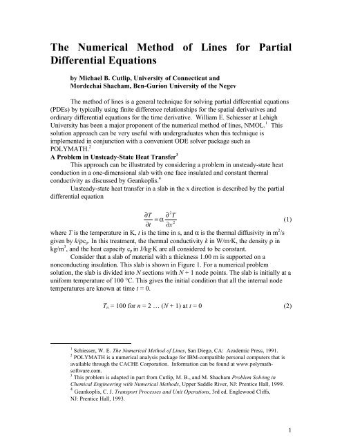
The Numerical Method of Lines for Partial Differential Equations

The Numerical Method of Lines for Partial 

Differential Equations 

by Michael B. Cutlip, University of Connecticut and 

Mordechai Shacham, Ben-Gurion University of the Negev 

The method of lines is a general technique for solving partial differential equations 

(PDEs) by typically using finite difference relationships for the spatial derivatives and 

ordinary differential equations for the time derivative. William E. Schiesser at Lehigh 

University has been a major proponent of the numerical method of lines, NMOL. 1 This 

solution approach can be very useful with undergraduates when this technique is 

implemented in conjunction with a convenient ODE solver package such as 

POLYMATH. 2 

A Problem in Unsteady-State Heat Transfer 3 

This approach can be illustrated by considering a problem in unsteady-state heat 

conduction in a one-dimensional slab with one face insulated and constant thermal 

conductivity as discussed by Geankoplis. 4 

Unsteady-state heat transfer in a slab in the x direction is described by the partial 

differential equation 

2 

∂T 

∂ T 

= α (1) 

2 

∂t 

∂x 

where T is the temperature in K, t is the time in s, and α is the thermal diffusivity in m 2 /s 

given by k/ρcp. In this treatment, the thermal conductivity k in W/m·K, the density ρ in 

kg/m 3 , and the heat capacity cp in J/kg·K are all considered to be constant. 

Consider that a slab of material with a thickness 1.00 m is supported on a 

nonconducting insulation. This slab is shown in Figure 1. For a numerical problem 

solution, the slab is divided into N sections with N + 1 node points. The slab is initially at a 

uniform temperature of 100 °C. This gives the initial condition that all the internal node 

temperatures are known at time t = 0. 

Tn = 100 for n = 2 … (N + 1) at t = 0 (2) 

1 Schiesser, W. E. The Numerical Method of Lines, San Diego, CA: Academic Press, 1991. 

2 POLYMATH is a numerical analysis package for IBM-compatible personal computers that is 

available through the CACHE Corporation. Information can be found at www.polymathsoftware.com. 

3 This problem is adapted in part from Cutlip, M. B., and M. Shacham Problem Solving in 

Chemical Engineering with Numerical Methods, Upper Saddle River, NJ: Prentice Hall, 1999. 

4 Geankoplis, C. J. Transport Processes and Unit Operations, 3rd ed. Englewood Cliffs, 

NJ: Prentice Hall, 1993. 

1

Figure 1 - Unsteady-State Heat Conduction in a One-dimensional Slab 

If at time zero the exposed surface is suddenly held constant at a temperature of 

0 °C, this gives the boundary condition at node 1: 

T1 = 0 for t ≥ 0 (3) 

The other boundary condition is that the insulated boundary at node N + 1 allows 

no heat conduction. Thus 

∂ TN + 1 

= 

0 for t ≥ 0 (4) 

∂x 

Note that this problem is equivalent to having a slab of twice the thickness exposed to the 

initial temperature on both faces. 

Problem (a) - Numerically solve Equation (1) with the initial and boundary 

conditions of (2), (3), and (4) for the case where α = 2 × 10 -5 m 2 /s and the slab 

surface is held constant at T1 = 0 °C. This solution should utilize the numerical 

method of lines with N = 10 sections. Plot the temperatures T2, T3, T4, and T5 as 

functions of time to 6000 s. 

For this problem with N = 10 sections of length Δx = 0.1 m, Equation (1) can be 

rewritten using a central difference formula for the second derivative as 

∂Tn 

α 

= ( T 1 2 

1 ) 

2 n+ 

− Tn 

+ Tn− 

for (2 ≤ n ≤ 10) (5) 

∂t 

( Δx) 

The boundary condition represented by Equation (4) can be written using a second-order 

backward finite difference as 

∂T 

∂t 

that can be solved for T11 to yield 

11 

= 

3T11 10 + T9 

T 

11 

− 4T 

2Δx 

= 0 

(6) 

4T10 − T9 

= (7) 

3 

2

The problem then requires the solution of Equations (3), (5), and (7) which 

results in nine simultaneous ordinary differential equations and two explicit algebraic 

equation for the 11 temperatures at the various nodes. This set of equations can be entered 

into the POLYMATH Simultaneous Differential Equation Solver or some other ODE 

solver. The resulting equation set for POLYMATH is 

Equations: 

d(T2)/d(t)=alpha/deltax^2*(T3-2*T2+T1) 









alpha=2.e-5 

T1=0 

T11=(4*T10-T9)/3 

deltax=.10 

The initial condition for each of the T’s is 100 and the independent variable t varies 

from 0 to 6000. The plots of the temperatures in the first four sections, node points 2 … 

5, are shown in Figure 2. The transients in temperatures show an approach to steady state. 

The numerical results are compared to the hand calculations of a finite difference solution 

by Geankoplis 4 (pp. 471–3) at the time of 6000 s in Table 1. These results indicate that 

there is general agreement regarding the problem solution, but differences between the 

temperatures at corresponding nodes increase as the insulated boundary of the slab is 

approached. 

Figure 2 – Temperature Profiles for Unsteady-state Heat Conduction in a 

One-dimensional Slab 

3

Table 1 – Results for Unsteady-state Heat Transfer in a One-dimensional 

Slab at t = 6000 s 

Distance 

Numerical Method of Lines 

from Slab Δx = 0.2m Δx = 0.1 m Δx = 0.05 m Δx = 0.0333 m 

Surface in m N = 5 N = 10 N = 20 N = 30 

n T n T n T n T 

0 1 0.0 1 0.0 1 0.0 1 0.0 

0.2 2 31.25 3 31.71 5 31.68 7 31.67 

0.4 3 58.59 5 58.49 9 58.47 13 58.47 

0.6 4 78.13 7 77.46 13 77.49 19 77.50 

0.8 5 89.84 9 88.22 17 88.29 25 88.31 

1.0 6 93.75 11 91.66 21 91.72 31 91.73 

Geankoplis 4 

Problem (b) - Repeat Problem (a) with 20 sections and compare results with part 

(a). 

The validity of the numerical solution can be investigated by doubling the number 

of sections for the NMOL solution. This involves adding an additional 10 equations given 

by the relationship in Equation (5), modifying Equation (7) to calculate T21, and halving 

Δx. The results for these changes in the POLYMATH equation set are also summarized in 

Table 1 as are similar results for 30 sections. Here the numerical solutions are similar to 

the previous solution in part (a) as the temperature profiles are virtually unchanged as the 

number of section is increased. 

Problem (c) - Repeat parts (a) and (b) for the case where heat convection is present 

at the slab surface. The heat transfer coefficient is h = 25.0 W/m 2 ·K, and the 

thermal conductivity is k = 10.0 W/m·K. 

When convection is considered as the only mode of heat transfer to the surface of 

the slab, an energy balance can be made at the interface that relates the energy input by 

convection to the energy output by conduction. Thus at any time for transport normal to 

the slab surface in the x direction 

∂T 

h ( T0 

− T1 

) = −k 

(8) 

∂x 

where h is the convective heat transfer coefficient in W/m 2 ·K and T0 is the ambient 

temperature. 

The preceding energy balance at the slab surface can be used to determine a 

relationship between the slab surface temperature T1, the ambient temperature T0, and the 

temperatures at internal node points. In this case, the second-order forward difference 

equation for the first derivative can be applied at the surface 

∂T 

∂x 

x= 

0 

= 

x= 

0 

( − T + T − 3T 

) 

3 

4 2 1 

2Δx 

(9) 

4

and can be substituted into Equation (8) to yield 

h( 

T 

0 

− T ) = −k 

The preceding equation can be solved for T1 to give 

T 

1 

= 

1 

( − T + 4T 

− 3T 

) 

3 

2 

2Δx 

2 2 

hT0Δx 

− kT3 

+ 4kT 

3k 

+ 2hΔx 

and the above equation can be used to calculate T1 during the NMOL solution. 

The resulting equation set for POLYMATH for Δx = 0.10 m for N = 10 is 

Equations: 










alpha=2.e-5 

deltax=.10 

T11=(4*T10-T9)/3 

h=25. 

T0=0 

k=10. 

T1=(2*h*T0*deltax-k*T3+4*k*T2)/(3*k+2*h*deltax) 

The preceding equation set can be integrated to any time t with POLYMATH or 

another ODE solver. The results at t = 1500 s are summarized in Table 2. 

Table 2 – Results for Unsteady-state Heat Transfer with Convection in a 

One-dimensional Slab at t = 1500 s 

Distance 

Numerical Method of Lines 

from Slab Δx = 0.2m Δx = 0.1 m Δx = 0.05 m Δx = 0.0333 m 

Surface in m N = 5 N = 10 N = 20 N = 30 

n T n T n T n T 

0 1 64.07 1 64.40 1 64.99 1 65.10 

0.2 2 89.07 3 88.13 5 88.77 7 88.90 

0.4 3 98.44 5 97.38 9 97.73 13 97.80 

0.6 4 100.00 7 99.61 13 99.72 19 99.74 

0.8 5 100.00 9 99.96 17 99.98 25 99.98 

1.0 6 100.00 11 100.00 21 100.00 31 100.00 

Geankoplis 4 

There is reasonable agreement between the various NMOL results as the number 

of sections (smaller Δx) is increased. The slower response of the temperatures within the 

1 

(10) 

(11) 

5

slab due to the additional convective resistance to heat transfer is evident when the 

temperatures are compared to those presented in Table 1. Selected temperatures are 

presented in Figure 3 for the same locations and at the same scale as Figure 2. The delays 

in the responses of the various temperatures are quite evident. 

Figure 3 – Temperature Profiles for Unsteady-state Heat Transfer with Convection 

in a One-dimensional Slab 

Problem Extensions 

There are a number of extensions to this problem that can be solved with the 

Numerical Method of Lines. The thermal conductivity of the solid could vary with the 

local temperature. There could be an initial temperature profile in the solid. Radiative heat 

transfer to the surface could be considered in addition to the convection. The convective 

heat transfer coefficient could be a function of the ΔT between the bulk gas and the slab 

surface. All these possibilities and more can be solved with the NMOL and an ODE 

solver such as POLYMATH. This type of problem can be used to effectively introduce 

undergraduate students to transient heat transfer and instruct them to the numerical 

solution of partial differential equations – a subject area that is not normally considered in 

a typical curriculum. 

6

The Numerical Method of Lines for Partial Differential Equations

You also want an ePaper? Increase the reach of your titles

Delete template?

Save as template?