Download - Polymath Software

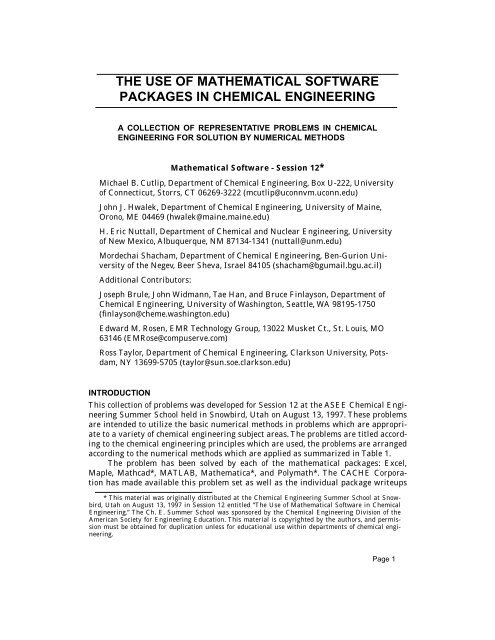
THE USE OF MATHEMATICAL SOFTWARE
PACKAGES IN CHEMICAL ENGINEERING
A COLLECTION OF REPRESENTATIVE PROBLEMS IN CHEMICAL
ENGINEERING FOR SOLUTION BY NUMERICAL METHODS
INTRODUCTION
Mathematical Software - Session 12*
Michael B. Cutlip, Department of Chemical Engineering, Box U-222, University
of Connecticut, Storrs, CT 06269-3222 (mcutlip@uconnvm.uconn.edu)
John J. Hwalek, Department of Chemical Engineering, University of Maine,
Orono, ME 04469 (hwalek@maine.maine.edu)
H. Eric Nuttall, Department of Chemical and Nuclear Engineering, University
of New Mexico, Albuquerque, NM 87134-1341 (nuttall@unm.edu)
Mordechai Shacham, Department of Chemical Engineering, Ben-Gurion University
of the Negev, Beer Sheva, Israel 84105 (shacham@bgumail.bgu.ac.il)
Additional Contributors:
Joseph Brule, John Widmann, Tae Han, and Bruce Finlayson, Department of
Chemical Engineering, University of Washington, Seattle, WA 98195-1750
(finlayson@cheme.washington.edu)
Edward M. Rosen, EMR Technology Group, 13022 Musket Ct., St. Louis, MO
63146 (EMRose@compuserve.com)
Ross Taylor, Department of Chemical Engineering, Clarkson University, Potsdam,
NY 13699-5705 (taylor@sun.soe.clarkson.edu)
This collection of problems was developed for Session 12 at the ASEE Chemical Engineering
Summer School held in Snowbird, Utah on August 13, 1997. These problems
are intended to utilize the basic numerical methods in problems which are appropriate
to a variety of chemical engineering subject areas. The problems are titled according
to the chemical engineering principles which are used, the problems are arranged
according to the numerical methods which are applied as summarized in Table 1.
The problem has been solved by each of the mathematical packages: Excel,
Maple, Mathcad*, MATLAB, Mathematica*, and Polymath*. The CACHE Corporation
has made available this problem set as well as the individual package writeups
* This material was originally distributed at the Chemical Engineering Summer School at Snowbird,
Utah on August 13, 1997 in Session 12 entitled “The Use of Mathematical Software in Chemical
Engineering.” The Ch. E. Summer School was sponsored by the Chemical Engineering Division of the
American Society for Engineering Education. This material is copyrighted by the authors, and permission
must be obtained for duplication unless for educational use within departments of chemical engineering.
Page 1

Page 2 MATHEMATICAL SOFTWARE PACKAGES IN CHEMICAL ENGINEERING
and problem solutions at http://www.che.utexas.edu/cache/. The materials are also available via anonymous
FTP from ftp.engr.uconn.edu in directory /pub/ASEE. The problem set and details of the various
solutions are given in separate documents as Adobe PDF files. Additionally, the problem sets are
available for the various mathematical package as working files which can be downloaded for execution
with the mathematical software. This method of presentation should indicate the convenience
and strengths/weaknesses of each of the mathematical software packages and provides working solutions.
The selection of problems has been coordinated by M. B. Cutlip who served as the session chairman.
The particular co-author who has considerable experience with a particular mathematical package
is responsible for the solution with that package*.
Excel** - Edward M. Rosen, EMR Technology Group
Maple** - Ross Taylor, Clarkson University
Mathematica** - H. Eric Nuttall, University of New Mexico
Mathcad** - John J. Hwalek, University of Maine
MATLAB** - Joseph Brule, John Widmann, Tae Han, and Bruce Finlayson, Department of
Chemical Engineering, University of Washington
POLYMATH** - Michael B. Cutlip, University of Connecticut and Mordechai Shacham, Ben-
Gurion University of the Negev
This selection of problems should help chemical engineering faculty evaluate which mathematical
problem solving package they wish to use in their courses and should provide some typical problems
in various courses which can be utilized.
* The CACHE Corporation is non-profit educational corporation supported by most chemical engineering departments
and many chemical corporation. CACHE stands for computer aides for chemical engineering. CACHE can be contacted at P.
O. Box 7939, Austin, TX 78713-7939, Phone: (512)471-4933 Fax: (512)295-4498, E-mail: cache@uts.cc.utexas.edu, Internet:
http://www.che.utexas.edu/cache/
** Excel is a trademark of Microsoft Corporation (http://www.microsoft.com), Maple is a trademark of Waterloo Maple,
Inc. (http://maplesoft.com), Mathematica is a trademark of Wolfram Research, Inc. (http://www.wolfram.com), Mathcad is a
trademark of Mathsoft, Inc. (http://www.mathsoft.com), MATLAB is a trademark of The Math Works, Inc. (http://www.mathworks.com),
and POLYMATH is copyrighted by M. B. Cutlip and M. Shacham (http://www.polymath-software.com).

Problem Selection
Page 3
Table 1 Selection of Problems Solutions Illustrating Mathematical Software
COURSE PROBLEM TITLE
Introduction to
Ch. E.
Introduction to
Ch. E.
Mathematical
Methods
Molar Volume and Compressibility Factor
from Van Der Waals Equation
Steady State Material Balances on a Separation
Train*
Vapor Pressure Data Representation by
Polynomials and Equations
Thermodynamics Reaction Equilibrium for Multiple Gas
Phase Reactions*
* Problem originally suggested by H. S. Fogler of the University of Michigan
** Problem preparation assistance by N. Brauner of Tel-Aviv University
MATHEMATICAL
MODEL PROBLEM
Single Nonlinear
Equation
Simultaneous Linear
Equations
Polynomial Fitting,
Linear and
Nonlinear Regression
Simultaneous
Nonlinear Equations
Fluid Dynamics Terminal Velocity of Falling Particles Single Nonlinear
Equation
Heat Transfer Unsteady State Heat Exchange in a
Series of Agitated Tanks*
Mass Transfer Diffusion with Chemical Reaction in a
One Dimensional Slab
Separation
Processes
Reaction
Engineering
Process Dynamics
and Control
Simultaneous
ODE’s with known
initial conditions.
Simultaneous
ODE’s with split
boundary conditions.
Binary Batch Distillation** Simultaneous Differential
and Nonlinear
Algebraic
Equations
Reversible, Exothermic, Gas Phase Reaction
in a Catalytic Reactor*
Dynamics of a Heated Tank with PI Temperature
Control**
Simultaneous
ODE’s and Algebraic
Equations
Simultaneous Stiff
ODE’s
These problem are taken in part from a new book entitled “Problem Solving in Chemical Engineering with Numerical
Methods” by Michael B. Cutlip and Mordechai Shacham to be published by Prentice-Hall in 1999.
1
2
3
4
5
6
7
8
9
10

Page 4 MATHEMATICAL SOFTWARE PACKAGES IN CHEMICAL ENGINEERING
1. MOLAR VOLUME AND COMPRESSIBILITY FACTOR FROM VAN
DER
WAALS
EQUATION
1.1 Numerical Methods
Solution of a single nonlinear algebraic equation.
1.2 Concepts Utilized
Use of the van der Waals equation of state to calculate molar volume and compressibility factor for a
gas.
1.3 Course Useage
Introduction to Chemical Engineering, Thermodynamics.
1.4 Problem Statement
The ideal gas law can represent the pressure-volume-temperature (PVT) relationship of gases only at
low (near atmospheric) pressures. For higher pressures more complex equations of state should be
used. The calculation of the molar volume and the compressibility factor using complex equations of
state typically requires a numerical solution when the pressure and temperature are specified.
The van der Waals equation of state is given by
where
and
The variables are defined by
P = pressure in atm
V = molar volume in liters/g-mol
a
P
V 2
⎛ +
⎝
------ ⎞( V – b)
= RT
⎠
a 27
-----
64
R2 2
⎛ Tc⎞ = ⎜------------- ⎟
⎝ Pc ⎠
b RTc =
----------
8Pc T = temperature in K
R = gas constant ( R = 0.08206 atm.
liter/g-mol.
K)
Tc
= critical temperature (405.5 K for ammonia)
Pc
= critical pressure (111.3 atm for ammonia)
(1)
(2)
(3)

Problem 1. MOLAR VOLUME AND COMPRESSIBILITY FACTOR FROM VAN DER WAALS EQUATION Page 5
Reduced pressure is defined as
and the compressibility factor is given by
Pr= P
-----
Pc Z PV
= --------
RT
(a) Calculate the molar volume and compressibility factor for gaseous ammonia at a pressure
P = 56 atm and a temperature T = 450 K using the van der Waals equation of state.
(b) Repeat the calculations for the following reduced pressures: P r = 1, 2, 4, 10, and 20.
(c) How does the compressibility factor vary as a function of P r .?
(4)
(5)

Page 6
MATHEMATICAL SOFTWARE PACKAGES IN CHEMICAL ENGINEERING
2. STEADY
STATE
MATERIAL
BALANCES
ON A SEPARATION
TRAIN
2.1 Numerical Methods
Solution of simultaneous linear equations.
2.2 Concepts Utilized
Material balances on a steady state process with no recycle.
2.3 Course Useage
Introduction to Chemical Engineering.
2.4 Problem Statement
Xylene, styrene, toluene and benzene are to be separated with the array of distillation columns that is
shown below where F, D, B, D1, B1, D2 and B2 are the molar flow rates in mol/min.
15% Xylene
25% Styrene
40% Toluene
20% Benzene
F=70 mol/min
Figure 1 Separation Train
D
#1
B
D 1
#2
B 1
D 2
#3
B 2
{
{
{
{
7% Xylene
4% Styrene
54% Toluene
35% Benzene
18% Xylene
24% Styrene
42% Toluene
16% Benzene
15% Xylene
10% Styrene
54% Toluene
21% Benzene
24% Xylene
65% Styrene
10% Toluene
1% Benzene

Problem 2. STEADY STATE MATERIAL BALANCES ON A SEPARATION TRAIN Page 7
Material balances on individual components on the overall separation train yield the equation set
Xylene: 0.07D
1
+ 0.18B
1
+ 0.15D
2
+ 0.24B
2
=
Styrene: 0.04D
1
+ 0.24B
1
+ 0.10D
2
+ 0.65B
2
=
Toluene: 0.54D
1
+ 0.42B
1
+ 0.54D
2
+ 0.10B
2
=
Benzene: 0.35D
1
+ 0.16B
1
+ 0.21D
2
+ 0.01B
2
=
0.15 × 70
0.25 × 70
0.40 × 70
Overall balances and individual component balances on column #2 can be used to determine the
molar flow rate and mole fractions from the equation of stream D from
Molar Flow Rates: D = D 1 + B 1
Xylene: X Dx D = 0.07D 1 + 0.18B 1
Styrene: X Ds D = 0.04D 1 + 0.24B 1
Toluene: X Dt D = 0.54D 1 + 0.42B 1
Benzene: X Db D = 0.35D 1 + 0.16B 1
0.20 × 70
where XDx
= mole fraction of Xylene, XDs
= mole fraction of Styrene, XDt
= mole fraction of Toluene,
and XDb
= mole fraction of Benzene.
Similarly, overall balances and individual component balances on column #3 can be used to
determine the molar flow rate and mole fractions of stream B from the equation set
Molar Flow Rates: B = D 2 + B 2
Xylene: X Bx B = 0.15D 2 + 0.24B 2
Styrene: X Bs B = 0.10D 2 + 0.65B 2
Toluene: X Bt B = 0.54D 2 + 0.10B 2
Benzene: X Bb B = 0.21D 2 + 0.01B 2
(a) Calculate the molar flow rates of streams D 1 , D 2 , B 1 and B 2 .
(b) Determine the molar flow rates and compositions of streams B and D.
(6)
(7)
(8)

Page 8 MATHEMATICAL SOFTWARE PACKAGES IN CHEMICAL ENGINEERING
3. VAPOR PRESSURE DATA REPRESENTATION BY POLYNOMIALS AND EQUATIONS
3.1 Numerical Methods
Regression of polynomials of various degrees. Linear regression of mathematical models with variable
transformations. Nonlinear regression.
3.2 Concepts Utilized
Use of polynomials, a modified Clausius-Clapeyron equation, and the Antoine equation to model vapor
pressure versus temperature data
3.3 Course Useage
Mathematical Methods, Thermodynamics.
3.4 Problem Statement
Table (2) presents data of vapor pressure versus temperature for benzene. Some design calculations
Table 2 Vapor Pressure of Benzene (Perry 3 )
Temperature, T
( o C)
Pressure, P
(mm Hg)
-36.7 1
-19.6 5
-11.5 10
-2.6 20
+7.6 40
15.4 60
26.1 100
42.2 200
60.6 400
80.1 760
require these data to be accurately correlated by various algebraic expressions which provide P in
mmHg as a function of T in °C.
A simple polynomial is often used as an empirical modeling equation. This can be written in general
form for this problem as
P a0a1T a2T2 a3T 3 ...+anT n
=
+ + + +
where a 0 ... a n are the parameters (coefficients) to be determined by regression and n is the degree of
the polynomial. Typically the degree of the polynomial is selected which gives the best data represen-
(9)

Problem 3. VAPOR PRESSURE DATA REPRESENTATION BY POLYNOMIALS AND EQUATIONS Page 9
tation when using a least-squares objective function.
The Clausius-Clapeyron equation which is useful for the correlation of vapor pressure data is
given by
log( P)
= A
B
– --------------------------
T + 273.15
where P is the vapor pressure in mmHg and T is the temperature in °C. Note that the denominator is
just the absolute temperature in K. Both A and B are the parameters of the equation which are typically
determined by regression.
The Antoine equation which is widely used for the representation of vapor pressure data is given
by
log( P)
= A
B
– --------------
T + C
where typically P is the vapor pressure in mmHg and T is the temperature in °C. Note that this equation
has parameters A, B, and C which must be determined by nonlinear regression as it is not possible
to linearize this equation. The Antoine equation is equivalent to the Clausius-Clapeyron equation
when C = 273.15.
(a) Regress the data with polynomials having the form of Equation (9). Determine the degree of
polynomial which best represents the data.
(b) Regress the data using linear regression on Equation (10), the Clausius-Clapeyron equation.
(c) Regress the data using nonlinear regression on Equation (11), the Antoine equation.
(10)
(11)

Page 10 MATHEMATICAL SOFTWARE PACKAGES IN CHEMICAL ENGINEERING
4. REACTION EQUILIBRIUM FOR MULTIPLE GAS PHASE REACTIONS
4.1 Numerical Methods
Solution of systems of nonlinear algebraic equations.
4.2 Concepts Utilized
Complex chemical equilibrium calculations involving multiple reactions.
4.3 Course Useage
Thermodynamics or Reaction Engineering.
4.4 Problem Statement
The following reactions are taking place in a constant volume, gas-phase batch reactor.
A+ B↔C+
D
B+ C↔X + Y
A+ X ↔ Z
A system of algebraic equations describes the equilibrium of the above reactions. The nonlinear
equilibrium relationships utilize the thermodynamic equilibrium expressions, and the linear relationships
have been obtained from the stoichiometry of the reactions.
K C1 =
CCC D
----------------
C ACB K C2 =
CX CY ----------------
CBC C
K C3 =
CZ ----------------
C AC X
C A = C A0 – CD – CZ CB = CB0 – CD – CY CC = CD – CY CY = CX + CZ In this equation set C A , CB , CC , CD , CX , CY and CZ are concentrations of the various species at
equilibrium resulting from initial concentrations of only CA0 and CB0 . The equilibrium constants KC1 ,
KC2 and KC3 have known values.
Solve this system of equations when CA0 = CB0 = 1.5, K C1 = 1.06 , K C2 = 2.63 and K C3 = 5
starting from four sets of initial estimates.
(a) CD = CX = CZ = 0
(b) CD = CX = CZ = 1
(c) CD = CX = CZ =
10
(12)

Problem 5. TERMINAL VELOCITY OF FALLING PARTICLES Page 11
5. TERMINAL VELOCITY OF FALLING PARTICLES
5.1 Numerical Methods
Solution of a single nonlinear algebraic equation..
5.2 Concepts Utilized
Calculation of terminal velocity of solid particles falling in fluids under the force of gravity.
5.3 Course Useage
Fluid dynamics.
5.4 Problem Statement
A simple force balance on a spherical particle reaching terminal velocity in a fluid is given by
where is the terminal velocity in m/s, g is the acceleration of gravity given by g = 9.80665 m/s 2 ,
is the particles density in kg/m3 , ρ is the fluid density in kg/m3 , is the diameter of the spherical
particle in m and CD is a dimensionless drag coefficient.
The drag coefficient on a spherical particle at terminal velocity varies with the Reynolds number
(Re) as follows (pp. 5-63, 5-64 in Perry3 vt ρ p
D p
).
C D
where Re = Dpvt ρ⁄ μ and μ is the viscosity in Pa⋅s or kg/m⋅s.
C D
v t
=
4 g( ρ p – ρ)Dp
------------------------------------
3CDρ 24
= ------ for Re < 0.1
Re
24
------ 1 0.14Re
Re
0.7
= ( + ) for 0.1 ≤ Re ≤ 1000
C D
= 0.44 for 1000 < Re ≤ 350000
4
CD = 0.19 – 8×10
⁄ Re for 350000 < Re
(a) Calculate the terminal velocity for particles of coal with ρp = 1800 kg/m3 and =
0.208×10-3 m falling in water at T = 298.15 K where ρ = 994.6 kg/m3 and μ = 8.931×10−4 D p
kg/
m⋅s.
(b) Estimate the terminal velocity of the coal particles in water within a centrifugal separator
where the acceleration is 30.0 g.
(13)
(14)
(15)
(16)
(17)

Page 12 MATHEMATICAL SOFTWARE PACKAGES IN CHEMICAL ENGINEERING
6. HEAT EXCHANGE IN A SERIES OF TANKS
6.1 Numerical Methods
Solution of simultaneous first order ordinary differential equations.
6.2 Concepts Utilized
Unsteady state energy balances, dynamic response of well mixed heated tanks in series.
6.3 Course Useage
Heat Transfer.
6.4 Problem Statement
Three tanks in series are used to preheat a multicomponent oil solution before it is fed to a distillation
column for separation as shown in Figure (2). Each tank is initially filled with 1000 kg of oil at 20°C.
Saturated steam at a temperature of 250°C condenses within coils immersed in each tank. The oil is
fed into the first tank at the rate of 100 kg/min and overflows into the second and the third tanks at
the same flow rate. The temperature of the oil fed to the first tank is 20°C. The tanks are well mixed so
that the temperature inside the tanks is uniform, and the outlet stream temperature is the temperature
within the tank. The heat capacity, Cp , of the oil is 2.0 KJ/kg. For a particular tank, the rate at
which heat is transferred to the oil from the steam coil is given by the expression
Q = UA( Tsteam – T)
where UA = 10 kJ/min·°C is the product of the heat transfer coefficient and the area of the coil for
each tank, T = temperature of the oil in the tank in °C , and Q = rate of heat transferred in kJ/min.
T 0 =20 o C
W 1 =100 kg/min
T 1
Steam
Figure 2 Series of Tanks for Oil Heating
T 2
Steam
Energy balances can be made on each of the individual tanks. In these balances, the mass flow
rate to each tank will remain at the same fixed value. Thus W = W 1 = W 2 = W 3 . The mass in each tank
will be assumed constant as the tank volume and oil density are assumed to be constant. Thus M = M 1
= M 2 = M 3 . For the first tank, the energy balance can be expressed by
Accumulation = Input - Output
T 3
Steam
T 1 T 2 T 3
dT1 MCp---------- =
WC
dt pT 0 + UA( Tsteam – T1) – WCpT 1
(18)
(19)

Problem 6. HEAT EXCHANGE IN A SERIES OF TANKS Page 13
Note that the unsteady state mass balance is not needed for tank 1 or any other tanks since the mass
in each tank does not change with time. The above differential equation can be rearranged and explicitly
solved for the derivative which is the usual format for numerical solution.
dT1 ---------- = [ WC
dt
p( T0 – T1) + UA( Tsteam – T1) ] ⁄ ( MCp) Similarly for the second tank
For the third tank
dT2 ---------- = [ WC
dt
p( T1 – T2) + UA( Tsteam – T2) ] ⁄ ( MCp) dT3 ---------- = [ WC
dt
p( T2 – T3) + UA( Tsteam – T3) ] ⁄ ( MCp) Determine the steady state temperatures in all three tanks. What time interval will be required
for T 3 to reach 99% of this steady state value during startup?
(20)
(21)
(22)

Page 14 MATHEMATICAL SOFTWARE PACKAGES IN CHEMICAL ENGINEERING
7. DIFFUSION WITH CHEMICAL REACTION IN A ONE DIMENSIONAL SLAB
7.1 Numerical Methods
Solution of second order ordinary differential equations with two point boundary conditions.
7.2 Concepts Utilized
Methods for solving second order ordinary differential equations with two point boundary values typically
used in transport phenomena and reaction kinetics.
7.3 Course Useage
Transport Phenomena and Reaction Engineering.
7.4 Problem Statement
The diffusion and simultaneous first order irreversible chemical reaction in a single phase containing
only reactant A and product B results in a second order ordinary differential equation given by
z 2
2
d C A k
= ----------- C
d
D A
AB
where C A is the concentration of reactant A (kg mol/m 3 ), z is the distance variable (m), k is the homogeneous
reaction rate constant (s -1 ) and D AB is the binary diffusion coefficient (m 2 /s). A typical geometry
for Equation (23) is that of a one dimension layer which has its surface exposed to a known
concentration and allows no diffusion across its bottom surface. Thus the initial and boundary conditions
are
C A
=
C A0 for z = 0
dC A
= 0 for z = L
(25)
dz
where CA0 is the constant concentration at the surface (z = 0) and there is no transport across the bottom
surface (z = L) so the derivative is zero.
This differential equation has an analytical solution given by
cosh[
L( k ⁄ DAB) ( 1 – z⁄ L)
]
C A =
C A0----------------------------------------------------------------------------
cosh(
L k⁄ DAB) (23)
(24)
(26)

Problem 7. DIFFUSION WITH CHEMICAL REACTION IN A ONE DIMENSIONAL SLAB Page 15
(a) Numerically solve Equation (23) with the boundary conditions of (24) and (25) for the case
where C A0 = 0.2 kg mol/m 3 , k = 10 -3 s -1 , D AB = 1.2 10 -9 m 2 /s, and L = 10 -3 m. This solution
should utilized an ODE solver with a shooting technique and employ Newton’s method or
some other technique for converging on the boundary condition given by Equation (25).
(b) Compare the concentration profiles over the thickness as predicted by the numerical solution
of (a) with the analytical solution of Equation (26).

Page 16 MATHEMATICAL SOFTWARE PACKAGES IN CHEMICAL ENGINEERING
8. BINARY BATCH DISTILLATION
8.1 Numerical Methods
Solution of a system of equations comprised of ordinary differential equations and nonlinear
algebraic equations.
8.2 Concepts Utilized
Batch distillation of an ideal binary mixture.
8.3 Course Useage
Separation Processes.
8.4 Problem Statement
For a binary batch distillation process involving two components designated 1 and 2, the moles of liquid
remaining, L, as a function of the mole fraction of the component 2, x2 , can be expressed by the following
equation
dL L
--------- = -------------------------
(27)
dx2 x2( k2 – 1)
where k2 is the vapor liquid equilibrium ratio for component 2. If the system may be considered ideal,
the vapor liquid equilibrium ratio can be calculated from ki = Pi ⁄ P where Pi is the vapor pressure of
component i and P is the total pressure.
A common vapor pressure model is the Antoine equation which utilizes three parameters A, B,
and C for component i as given below where T is the temperature in °C.
P i
⎛ B
A – -------------- ⎞
⎝ T + C⎠
= 10
The temperature in the batch still follow the bubble point curve. The bubble point temperature is
defined by the implicit algebraic equation which can be written using the vapor liquid equilibrium
ratios as
k1x 1 + k2x 2 =
1
Consider a binary mixture of benzene (component 1) and toluene (component 2) which is to be
considered as ideal. The Antoine equation constants for benzene are A 1 = 6.90565, B 1 = 1211.033 and
C 1 = 220.79. For toluene A 2 = 6.95464, B 2 = 1344.8 and C 2 = 219.482 (Dean 1 ). P is the pressure in mm
(28)
(29)

Problem 8. BINARY BATCH DISTILLATION Page 17
Hg and T the temperature in °C.
The batch distillation of benzene (component 1) and toluene (component 2) mixture is being carried
out at a pressure of 1.2 atm. Initially, there are 100 moles of liquid in the still, comprised of
60% benzene and 40% toluene (mole fraction basis). Calculate the amount of liquid remaining in
the still when concentration of toluene reaches 80%.

Page 18 MATHEMATICAL SOFTWARE PACKAGES IN CHEMICAL ENGINEERING
9. REVERSIBLE, EXOTHERMIC, GAS PHASE REACTION IN A CATALYTIC REACTOR
9.1 Numerical Methods
Simultaneous ordinary differential equations with known initial conditions.
9.2 Concepts Utilized
Design of a gas phase catalytic reactor with pressure drop for a first order reversible gas phase reaction.
9.3 Course Useage
Reaction Engineering
9.4 Problem Statement
The elementary gas phase reaction 2 A C is carried out in a packed bed reactor. There is a heat
exchanger surrounding the reactor, and there is a pressure drop along the length of the reactor.
F A0
T 0
The various parameters values for this reactor design problem are summarized in Table (3).
Table 3 Parameter Values for Problem 9.
C PA = 40.0 J/g-mol . K R = 8.314 J/g-mol . K
C PC = 80.0 J/g-mol . K F A0 = 5.0 g-mol/min
= - 40,000 J/g-mol Ua = 0.8 J/kg . min . K
EA = 41,800 J/g-mol . K Ta = 500 K
k = 0.5 dm 6 /kg⋅min⋅mol @ 450 K = 0.015 kg -1
ΔH
R
α
K C = 25,000 dm 3 /g-mol @ 450 K P 0 = 10 atm
C A0 = 0.271 g-mol/dm 3 y A0 = 1.0 (Pure A feed)
T 0 = 450 K
T a
q
T a
Figure 3 Packed Bed Catalytic Reactor
q
X
T

Problem 9. REVERSIBLE, EXOTHERMIC, GAS PHASE REACTION IN A CATALYTIC REACTOR Page 19
(a) Plot the conversion (X), reduced pressure (y) and temperature (T ×10 -3 ) along the reactor
from W = 0 kg up to W = 20 kg.
(b) Around 16 kg of catalyst you will observe a “knee” in the conversion profile. Explain why this
knee occurs and what parameters affect the knee.
(c) Plot the concentration profiles for reactant A and product C from W = 0 kg up to W = 20 kg.
Addition Information
The notation used here and the following equations and relationships for this particular problem are
adapted from the textbook by Fogler. 2 The problem is to be worked assuming plug flow with no radial
gradients of concentrations and temperature at any location within the catalyst bed. The reactor
design will use the conversion of A designated by X and the temperature T which are both functions of
location within the catalyst bed specified by the catalyst weight W.
The general reactor design expression for a catalytic reaction in terms of conversion is a mole
balance on reactant A given by
dX
F A0---------
= – r'
dW A
The simple catalytic reaction rate expression for this reversible reaction is
– r' A k C2 A
where the rate constant is based on reactant A and follows the Arrhenius expression
CC = – --------
K C
The stoichiometry for 2 A C and the stoichiometric table for a gas allow the concentrations to
be expressed as a function of conversion and temperature while allowing for volumetric changes due
to decrease in moles during the reaction. Therefore
and
E A
k = k( @T=450°K ) exp-------
R
1 1
-------- – ---
450 T
and the equilibrium constant variation with temperature can be determined from van’t Hoff’s equation
with C
(33)
˜ Δ P = 0
K C =
ΔH
R
K C( @T=450°K ) exp------------
R
1 1
-------- – ---
450 T
C A
C ⎛ 1 – X
A0 ---------------- ⎞ P
------
⎝1+ εX⎠P0
T0 1 – X T
------ C ⎛
T A0 --------------------- ⎞ 0
= =
y------ ⎝1– 0.5 X⎠
T
y
=
P
------
P0 0.5C A0 X T
C ⎛
C ----------------------- ⎞ 0
=
y------ ⎝ 1 – 0.5 X ⎠ T
(30)
(31)
(32)
(34)
(35)

or
Page 20 MATHEMATICAL SOFTWARE PACKAGES IN CHEMICAL ENGINEERING
The pressure drop can be expressed as a differential equation (see Fogler 2 for details)
d P ⎛------ ⎞
⎝P⎠ 0 – α( 1 + εX )
-----------------------------------------dW 2
P0 ------
P
T
=
------
T0 dy
-------dW
The general energy balance may be written at
– α( 1 – 0.5 X )
---------------------------------
2 y
T
=
------
T0 dT
--------dW
Ua Ta T – ( ) r' A H + ( Δ R)
F A0 θiC Pi X C˜ = --------------------------------------------------------------
( + Δ P)
which for only reactant A in the reactor feed simplifies to
∑
dT
--------dW
Ua Ta T – ( ) r' A H + ( Δ R)
=
--------------------------------------------------------------
F A0( CPA) (36)
(37)
(38)
(39)

Problem 10. DYNAMICS OF A HEATED TANK WITH PI TEMPERATURE CONTROL Page 21
10. DYNAMICS OF A HEATED TANK WITH PI TEMPERATURE CONTROL
10.1 Numerical Methods
Solution of ordinary differential equations, generation of step functions, simulation of a proportional
integral controller.
10.2 Concepts Utilized
Closed loop dynamics of a process including first order lag and dead time. Padé approximation of time
delay.
10.3 Course Useage
Process Dynamics and Control
10.4 Problem Statement
A continuous process system consisting of a well-stirred tank, heater and PI temperature controller is
depicted in Figure (4). The feed stream of liquid with density of ρ in kg/m 3 and heat capacity of C in
kJ / kg⋅°C flows into the heated tank at a constant rate of W in kg/min and temperature Ti in °C. The
volume of the tank is V in m3 . It is desired to heat this stream to a higher set point temperature Tr in
°C. The outlet temperature is measured by a thermocouple as Tm in °C, and the required heater input
q in kJ/min is adjusted by a PI temperature controller. The control objective is to maintain T0 = Tr in
the presence of a change in inlet temperature Ti which differs from the steady state design temperature
of Tis .
Feed
W, T i , ρ, C p
Heater TC
q
V, T
PI
controller
Thermocouple
Measured
Tm Set point
T r
W, T 0 , ρ, C p
Figure 4 Well Mixed Tank with Heater and Temperature Controller

Page 22 MATHEMATICAL SOFTWARE PACKAGES IN CHEMICAL ENGINEERING
Modeling and Control Equations
An energy balance on the stirred tank yields
dT
------- (40)
dt
with initial condition T = Tr at t = 0 which corresponds to steady state operation at the set point temperature
Tr ..
The thermocouple for temperature sensing in the outlet stream is described by a first order system
plus the dead time τd which is the time for the output flow to reach the measurement point. The
dead time expression is given by
WCp Ti T – ( ) q +
= -------------------------------------------ρVCp
The effect of dead time may be calculated for this situation by the Padé approximation which is a first
order differential equation for the measured temperature.
dT0 ---------- = T – T
dt
0
τ
⎛ d
----- ⎞ dT
– ⎛------- ⎞
⎝ 2 ⎠⎝
dt⎠
(41)
I. C. T 0 = T r at t = 0 (steady state) (42)
The above equation is used to generated the temperature input to the thermocouple, T 0 .
The thermocouple shielding and electronics are modeled by a first order system for the input
temperature T 0 given by
dTm -----------dt
T0 – Tm = --------------------τm
I. C. T m = T r at t = 0 (steady state) (43)
where the thermocouple time constant τ m is known.
The energy input to the tank, q, as manipulated by the proportional/integral (PI) controller can
be described by
where K c is the proportional gain of the controller, τ I is the integral time constant or reset time. The q s
in the above equation is the energy input required at steady state for the design conditions as calculated
by
The integral in Equation (44) can be conveniently be calculated by defining a new variable as
d
( errsum)
= Tr – T
dt
m
Thus Equation (44) becomes
T0() t = T( t– τd) 2
----τd
q qsKc( Tr – Tm) K c t
= + + ------ ( T
τ r – Tm) dt
0
I
(44)
(45)
I. C. errsum = 0 at t = 0 (steady state) (46)
q qsKc( Tr – Tm) (47)
Let us consider some of the interesting aspects of this system as it responds to a variety of parameter
K c
=
+ + ------ ( errsum)
τI ∫
qs = WCp( Tr – Tis)

Page 23 MATHEMATICAL SOFTWARE PACKAGES IN CHEMICAL ENGINEERING
and operational changes.The numerical values of the system and control parameters in Table (4) will
be considered as leading to baseline steady state operation.
Table 4 Baseline System and Control Parameters for Problem 10
ρVC p = 4000 kJ/°C WC p = 500 kJ/min⋅°C
T is = 60 °C T r = 80 °C
τ d = 1 min τ m = 5 min
K c = 50 kJ/min⋅°C τ I = 2 min
(a) Demonstrate the open loop performance (set K c = 0) of this system when the system is initially
operating at design steady state at a temperature of 80°C, and inlet temperature T i is suddenly
changed to 40°C at time t = 10 min. Plot the temperatures T, T 0 , and T m to steady state,
and verify that Padé approximation for 1 min of dead time given in Equation (42) is working
properly.
(b) Demonstrate the closed loop performance of the system for the conditions of part (a) and the
baseline parameters from Table (4). Plot temperatures T, T 0 , and T m to steady state.
(c) Repeat part (b) with K c = 500 kJ/min⋅°C.
(d) Repeat part (c) for proportional only control action by setting the term K c /τ I = 0.
(e) Implement limits on q (as per Equation (47)) so that the maximum is 2.6 times the baseline
steady state value and the minimum is zero. Demonstrate the system response from baseline
steady state for a proportional only controller when the set point is changed from 80°C to 90°C at
t = 10 min. K c = 5000 kJ/min⋅°C. Plot q and q lim versus time to steady state to demonstrate the limits.
Also plot the temperatures T, T 0 , and T m to steady state to indicate controller performance

Page 24 MATHEMATICAL SOFTWARE PACKAGES IN CHEMICAL ENGINEERING
REFERENCES
1. Dean, A. (Ed.), Lange’s Handbook of Chemistry, New York: McGraw-Hill, 1973.
2. Fogler, H. S. Elements of Chemical Reaction Engineering, 2nd ed., Englewood Cliffs, NJ: Prentice-Hall,
1992.
3. Perry, R.H., Green, D.W., and Malorey, J.D., Eds. Perry’s Chemical Engineers Handbook. New York:
McGraw-Hill, 1984.
4. Shacham, M., Brauner; N., and Pozin, M. Computers Chem Engng., 20, Suppl. pp. S1329-S1334 (1996).