Nonideal Reactor Design using POLYMATH - Polymath Software
Nonideal Reactor Design using POLYMATH - Polymath Software
Nonideal Reactor Design using POLYMATH - Polymath Software

Create successful ePaper yourself
Turn your PDF publications into a flip-book with our unique Google optimized e-Paper software.
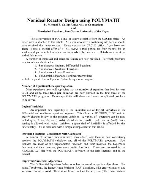
<strong>Nonideal</strong> <strong>Reactor</strong> <strong>Design</strong> <strong>using</strong> <strong>POLYMATH</strong><br />
by Michael B. Cutlip, University of Connecticut<br />
and<br />
Mordechai Shacham, Ben-Gurion University of the Negev<br />
The latest version of <strong>POLYMATH</strong> is now available from the CACHE office. An<br />
order form is attached to this article. All users who have a continuing site license should<br />
have received this latest version. Please contact the CACHE office if you have not.<br />
There is also a special offer of a <strong>POLYMATH</strong> trial period for four months for an<br />
academic department before a site license needs to be purchased. Details are also at the<br />
end of this article.<br />
A number of improved and enhanced feature are now provided. <strong>Polymath</strong> programs<br />
now include capabilities for<br />
1. Simultaneous Ordinary Differential Equations<br />
2. Simultaneous Nonlinear Equations<br />
3. Simultaneous Linear Equations<br />
4. Polynomial, Linear and Nonlinear Regressions<br />
with the separate Linear Equation Solver being a new program.<br />
Number of Equations/Lines per Equation<br />
Most experience users will appreciate that the number of equations has been increase<br />
to 31 and up to three lines per equation are now allowed in the first three of the<br />
<strong>POLYMATH</strong> programs. These capabilities will allow much more complicated problems<br />
to be solved.<br />
Logical Variables<br />
An important new capability is the unlimited use of logical variables in the<br />
differential and nonlinear equations programs. This allows an IF, THEN, ELSE logic to<br />
specify changes in any of the program variables. A variety of operators can be used<br />
including >, =,
precision). The program will decrease the step size in order to achieve a relative and<br />
absolute error or 10 -10 if possible. If the accuracy become less than 10 -4 , then the user<br />
can choose a "semi-implicit midpoint rule" which is an algorithm for stiff problems.<br />
Expanded Statistical Output for Regressions<br />
More statistical information is now provided in the various regressions involving<br />
polynomials, multiple linear functions and general nonlinear functions. This includes the<br />
matrix of correlation coefficients, the 95% confidence intervals for all parameters, and the<br />
overall variance. This can be quite useful in deciding which model should be retained and<br />
used to correlate data.<br />
Improved Graphical Output and Support for Printers, Plotters and Graphics Files<br />
Most of the graphical results can be edited to change the scales of the x and y axes,<br />
to label the x and y axes, and to title the graph. Normal printing is to a variety of some 30<br />
standard printers and six plotters. Advanced printing options provide a variety of standard<br />
graphical file types for incorporation into documents.<br />
Example of Logical Variable Use - Non Ideal <strong>Reactor</strong> <strong>Design</strong> Using Residence Time<br />
Distribution Functions<br />
Non ideal reactor design for segregated flow involves the solution of<br />
_<br />
∞<br />
∫ 0<br />
C = E( t) C ( t) dt<br />
A A<br />
where E(t) is the residence time distribution function (RTD) and C A (t) is the<br />
concentration from a batch reactor at time t. CA is the calculated outlet concentration.<br />
The above integral equation can be written in differential equation form as<br />
dC A<br />
= E( t) C A ( t)<br />
dt<br />
I. C. = 0 at t = 0 (2)<br />
for evaluation by <strong>POLYMATH</strong> when the E(t) function is known. Integration is carried<br />
out to large values of t where the resulting outlet concentration CA no longer changes<br />
with time.<br />
For a laminar flow reactor the RTD is given by E( t)<br />
=<br />
t<br />
τ τ<br />
when t ≥ else it is<br />
3<br />
2 2<br />
zero. Here τ (tau) is the mean residence time of the reactor given by V/v<br />
0<br />
. The RTD<br />
function for laminar flow can be entered <strong>using</strong> the <strong>POLYMATH</strong> if, then, or else logical<br />
variable statement.<br />
EoftLAMINAR = if (t) >= tau/2.) then (tau^2/(2.*t^3) else (0.0)<br />
Let us consider a second order, irreversible, liquid phase reaction occurring within<br />
the laminar flow reactor <strong>using</strong> the RTD function. This can easily be handled in<br />
_<br />
_<br />
(1)<br />
2
<strong>POLYMATH</strong> by numerically solving the differential equation for the batch reactor given<br />
by<br />
dC A<br />
2<br />
= −kC<br />
I. C. C<br />
A<br />
= 1.0 at t = 0 (3)<br />
dt<br />
A<br />
during the during the simultaneous integration of the RTD differential equation (2) for<br />
CA . The initial condition (I. C.) on CA is considered to be 1.0<br />
The <strong>POLYMATH</strong> equations for the case where k = 0.2 and tau=5.0 are shown<br />
below in Figure 1 as they appear on the screen prior to solution.<br />
Figure 1 - <strong>Polymath</strong> Code for Laminar Flow <strong>Reactor</strong><br />
The scaled and titled <strong>POLYMATH</strong> plot for the laminar flow reactor is shown in<br />
Figure 2. Note that the calculated concentration is approaching a constant value at t = 30.<br />
Figure 2 - Graphical Output of the Conversion for Laminar Flow <strong>Reactor</strong><br />
The RTD curve for the laminar flow reactor can also be plotted after the numerical<br />
solution has been obtained. This is shown in Figure 3 which nicely shows the<br />
breakthrough of the RTD curve at one half of the mean residence time where tau = 2.5.<br />
3
Figure 3 - RTD for Laminar Flow <strong>Reactor</strong><br />
This simple example shows the usefulness of the logical variable capability with<br />
<strong>POLYMATH</strong>. This problem involving segregated flow modeling can easily be expanded<br />
to include the RTD functions for various ideal reactors and experimental RTD’s for real<br />
reactors as polynomial expressions. This is treated in the next section of this article.<br />
How to Compare Simulations Easily within <strong>POLYMATH</strong><br />
The previous example can be extended to other reactors when the RTD functions<br />
are known or can be measured. Some of the commonly used ideal reactor RTD for the<br />
plug flow, CSTR and series of N CSTR’s are given below:<br />
EoftPLUG=if((t)=.99*tau)&(t
Figure 4 - RTD Treatment for Various Ideal <strong>Reactor</strong>s with Second Order Reaction<br />
The Partial Results Table from the <strong>POLYMATH</strong> solution shown in Figure 5 gives<br />
general information on various problem variables before the user is prompted for various<br />
plots or tabular output.<br />
Figure 5 - Partial Results Table Generated by <strong>POLYMATH</strong><br />
The graphical results of all four reactors are presented in Figure 6 as generated<br />
directly by <strong>POLYMATH</strong>. Note that the solution does not change for times greater than<br />
30 where the solution for each of the various reactors is asymptotically approached. Thus<br />
summarized values of the predicted outlet concentrations given in Figure 5 are reasonable.<br />
Of course, the integration could be continued to larger time to confirm this. As expected,<br />
the calculated concentrations decrease according to the reactor types - CSTR, Laminar<br />
Flow, N-CSTR, and Plug Flow. The conversion increase according to the same order.<br />
Note that the N-CSTR with N = 10 approaches that of the Plug Flow reactor. This could<br />
also be calculated with larger values of N by rerunning the <strong>POLYMATH</strong> program.<br />
5
Figure 6 - RTD Solution for Average Concentrations Exiting Various Ideal <strong>Reactor</strong>s<br />
The RTD curves for the various reactors can also be plotted at the request of the<br />
user. These are shown in Figure 7 where the characteristics of the various reactors can<br />
easily be compared.<br />
Figure 7 - RTD Functions for Various Ideal <strong>Reactor</strong>s<br />
In summary, the new version 4.0 of <strong>POLYMATH</strong> has new capabilities that greatly<br />
enhance the usefulness of the software. Student users find the software particularly easy<br />
to learn to use. There is no risk in evaluating this software. The inexpensive site license<br />
allows unlimited copying of the software for educational use by students, faculty and staff.<br />
and its use in Chemical Engineering.<br />
6