Efficient Solution of Numerical Problems within Polymath and Excel

Efficient Solution of Numerical Problems within Polymath and Excel
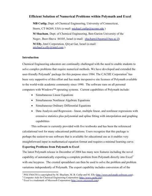
Introduction
MB Cutlip, Dept. of Chemical Engineering, University of Connecticut,
Storrs, CT 06269, USA (e-mail: michael.cutlip@uconn.edu )
M Shacham, Dept. of Chemical Engineering, Ben-Gurion University of the
Negev, Beer-Sheva 84105, Israel (e-mail: shacham@bgumail.bgu.ac.il)
M Elly, Intel Corporation, Qiryat Gat, Israel (e-mail:
michael.a.elly@intel.com )
Chemical Engineering educators are continually challenged with the need to enable students to
solve complex problems that require numerical methods. We have developed and extended the
user-friendly Polymath 1 package for this purpose since 1984. The CACHE Corporation 2 has
been very supportive of this effort and has made inexpensive site licenses of Polymath available
to the world-wide academic community since 1990. The software runs on all personal
computers with Windows operating systems. Current capabilities of Polymath include:
• Simultaneous Linear Equations
• Simultaneous Nonlinear Algebraic Equations
• Simultaneous Ordinary Differential Equations
• Data Analysis and Regression - linear, multiple linear, and nonlinear regressions with
extensive statistics plus polynomial and spline fitting with interpolation and graphing
capabilities
This software is currently provided with five textbooks and has been the referenced
calculational tool for many educational publications. Users recognize that this package is
perhaps the easiest-to-use software that is available for educational use as it enables very
straightforward input in mathematical equation format and requires a minimal learning curve.
Exporting Problems from Polymath to Excel
The latest Polymath release in December of 2004 has many new features including the novel
capability of automatically exporting a complete problem from Polymath directly into Excel 3
with one keypress. The created spreadsheet can then be used to solve the problem and problem
variations independently of Polymath. The export capability includes conversion all of the
1 POLYMATH is copyrighted by M. Shacham, M. B. Cutlip and M. Elly (http://www.polymath-software.com).
2 Computer Aids for Chemical Engineering Corporation (http://www.cache.org).
3 Excel is a trademark of Microsoft Corporation (http://www.microsoft.com).

intrinsic functions and logical functionality found within Polymath. Within Excel, the “Solver”
Add-In is used for nonlinear equations and nonlinear regressions. The LINEST functionality in
Excel is used for linear regressions. For differential equations, we have created an Ode_Solver
Add-In for Excel that numerically integrates simultaneous ordinary differential equations.
This software provides educators and their students with problem solving capabilities for
a numerical computation package (Polymath) and also a spreadsheet package (Excel). Thus
students become familiar with both of these environments. Most importantly, this enables more
complex and realistic problems to be posed and easily solved in chemical engineering education.
Incorporation of Physical Property Data in Excel
A recent addition to the capabilities within Excel is the availability of the Aspen Properties
Add-In from AspenTech 4 that gives users access to advanced physical property data during
problem solving within Excel. This capability of calling upon realistic physical properties
during student problem solving may well represent an important new paradigm in Chemical
Engineering Education.
An Example Problem - Cocurrent Operation of a Double Pipe Heat Exchanger
The usefulness of Polymath, Excel, and Aspen Properties will be illustrated with the following
problem involving a double pipe heat exchanger from Cutlip, M. B. and M. Shacham (1).
Consider a concurrent double pipe heat exchanger with cooling water in the shell side
and benzene in the tube side. The cooling water is available at 65 °F and has a flow that is three
times that of the benzene. The inlet benzene temperature is 150 °F. The configuration of the
heat exchanger is given below in Figure 1.
Figure 1 – Double Pipe Heat Exchanger
4 Aspen Properties is a registered product of AspenTech (http://www.aspentech.com).
2

Equation (1) represents the local heat transfer coefficient where the exponent n = 0.4 for
heating and 0.3 for cooling.
The local overall heat transfer coefficient based on the inside area can be calculated from
Geankoplis (2)
where t represents the tube wall material and dimensions. The Dtlm term is the log mean
diameter (or area) for the tube wall.
A differential energy balance on the benzene streawm in the tube yields the following
differential equation where the prime indicates that the benzene properties are to be evaluated at
the local temperature of the benzene.
Similarly for the insulated shell side, a differential energy balance yields the following
differential equation where the physical properties of water are to be evaluated at the local
temperature of the water.
Solution of Sample Problem
This sample problem will be solved in three ways:
1) The Polymath program will be used to solve the problem for the case where the physical
properties are assumed to be constant at the inlet temperatures to the heat exchanger.
2) The exported problem from Polymath to Excel will be solved completely within Excel
using the Polymath Ode_Solver Add-In.
3) The problem in Excel will be solved with the physical properties provided by the Aspen
Properties Excel Add-In, and the solution of the differential equations will use the
Polymath Ode_Solver Add-In.
Polymath Program Solution – Constant Physical Properties
The entry of this problem into the Polymath editor for the Differential Equations Solver is
shown in Figure 1. Note that the equations can be entered in any order as Polymath will order
the equations before solution. The equations with the comments contain the physical property
variables that are entered as constants in this program at the initial temperatures for simplicity.
3
(1)
(2)
(3)
(4)

Figure 1 – Polymath Editing Display for Sample Problem (Differential Equation Sover)
The solution of this problem with a single mouse click on the purple arrow icon in
Polymath yields a ‘Report’ in which general information regarding the solution is provided.
Many other options are available including graphical and tabular output. Portions of the ‘Report’
are reproduced in Figure 2. Note that the initial value, minimal value, maximal value, and final
value of all the problem variables are summarized in this ‘Report’. In addition, the various
differential equations and the explicit equations are also given. The complete ordered equation
set with the comments is also provided (not shown in the figure).
4

Figure 2 – Partial Screen Display of Polymath Report
Polymath Export to Excel
This problem can be exported from the Polymath Differential Equations Editor to Excel with a
single keypress. During this automatic export process, all the intrinsic functions and logical
variables are converted to their equivalents in the code for the spreadsheet. Once any problem
has been exported to Excel, the numerical solutions can be completely accomplished within
Excel. The Excel "Solver" can be used for solving nonlinear algebraic equations. Regression
problems utilize the Excel “LINEST” function or “Solver”. For systems of ODE’s (ordinary
differential equations), the Polymath Ode_Solver Add-In for Excel must be used.
The resulting Excel worksheet is shown in Figure 3. In the Excel worksheet, the variable
names, the Polymath equations, and the comments are shown for documentation purposes. The
Excel formulas are generated and placed in the 3 rd column, marked as "Value". They are
transparent to the user unless he/she asks explicitly to see them. The formula to calculate
d(TH2O)/d(x) for example is:
d(TH2O)/d(x) = ((((C27 * 3.1416) * C3) * (C29 - C28)) / (C12 * C13))
5

Figure 3 – Exported Program from Polymath to Excel
Thus the exported problem is ready for solution within Excel.
Excel Solution – Constant Physical Properties
The Polymath Ode_Solver Add-In that has been developed to work independently within Excel.
It is an Add-In just like ‘Solver” which is supplied with Excel for solving nonlinear equations.
The Ode_Solver requires input of the following cell addresses and numerical values: 1) The
range of the cells where the initial values of the differential equations are stored; 2) The range of
the cells where the formulas of the differential equations are stored; 3) The cell where the initial
value for the independent variable (time, in this case) is stored; 4) The final value of the
independent variable; 5) The range of cells where formulas of additional variables for which the
integration results should be stored (optional).
Solution of the differential equations is implemented by clicking on the Ode_Solver in the
‘Tools’ menu of Excel. This brings up the display shown in Figure 4 where the various input
cells have been identified. Note that 101 data points have been requested for this problem which
can be used for graphical presentation of the results. No other variables have been specified.
The Adv. button allows selection of a particular integration algorithm and its parameters.
6

Figure 4 – Ode_Solver Input Window within Sample Problem
During the real-time solution of the differential equations within Excel, the cells with the
blue titles (Integration Vars, ODE EQS, and Indep Var) in column C of Figure 3 change as the
integration proceeds. A new worksheet is then created in the Excel workbook that contains a
‘Report’ of the problem solution. This is partly shown in Figure 5, although the table of
variables is not shown but is always generated within this Excel solution ’Report’. The
‘Reports’ of Figure 2 (Polymath Solution) and Figure 5 (Excel Solutions) are exactly equivalent.
Figure 5 – Partial View of Excel Spreadsheet Giving Problem Report Information
7

Excel Solution – Variable Physical Properties
The variation of the physical properties of the benzene and water in this sample problem can be
accommodated with the Aspen Properties Add-In for Excel. This first requires that the system
of components be entered into the Aspen Properties program which is a part of the Aspen
Engineering Suite. The then allows the user to setup a location within the Excel spreadsheet that
can link the spreadsheet to Aspen Properties as shown in Figure 6. The Aspen file is colored
purple in the spreadsheet.
Figure 6 – Aspen Properties Link in Excel
This portion of the spreadsheet responds to changes in temperature and pressure by updating the
contents of the cells that contain the physical properties data.
The physical property data can be integrated together with the problem solution by
copying the exported worksheet from Polymath to Excel with the constant physical properties
shown in Figure 3 to the worksheet in Figure 6. This integrated spreadsheet is presented in
Figure 7. Note that some conversion factors have been entered into the cell where the physical
properties are found to achieve consistency in the units. The highlighted rows in Figure 7
indicate the property variables that vary with temperature. As the value of the water
temperature in cell C42 changes, then all of the properties of water change. As the value of the
benzene temperature in cell C43 changes, then the properties of benzene adjust accordingly.
Thus all of the other equations are updated as these temperatures change during the course of the
numerical integration of the differential equations.
8

Figure 7 – Integrated Aspen Properties and Polymath to Excel Spreadsheet
Figure 8 - Partial Report for Excel Solution with Variable Physical Properties
It is interesting to compare the results from the solution with constant physical properties
given in Figure 2 with the solution with variable physical properties given in Figure 8. The
benzene outlet temperature is about 0.6 °F higher and the water outlet temperature is about 1.8
°F higher.
9

Conclusions
1) The Polymath package provides problem solving software on personal computers that
can be widely utilized in Chemical Engineering Education. The latest version includes
options for easily exporting problems to Excel for execution directly within the
spreadsheet.
2) The Polymath Ode_Solver for Excel, available as an Add-In, allows the convenient
solution of systems of ordinary differential equations within a spreadsheet. This will
allow more advanced problem solving among both students and professional engineers
as the Excel software is quite widely used.
3) Physical property data can be introduced into problem solving in Excel through the use
of the Aspen Properties Add-In. This provides access to the extensive physical property
data bases of the Aspen Engineering Suite.
4) The use of problem solving with convenient access to physical property data has the
References
potential to become a new paradigm in Chemical Engineering Education. The
introduction of this capability to beginning students will greatly impact the ways in
which problems will be posed and solved throughout the curriculum. It will allow more
realistic problems to be posed and efficiently solved throughout the educational program
of chemical engineers. It has the potential to be quite valuable in their professional
engineering careers.
1. Cutlip, M. B. and M. Shacham, Problem Solving in Chemical Engineering with
Numerical Methods, Prentice Hall, Upper Saddle River, NJ, 1998.
2. Geankoplis, C. J., Transport Processes and Separation Process Principles, 4 th ed.,
Prentice Hall, Upper Saddle River, NJ, 2003.
10