polymath solutions to the chemical engineering problem set

POLYMATH SOLUTIONS TO THE CHEMICAL 

ENGINEERING PROBLEM SET 

Mathematical Software - Session 12* 

Michael B. Cutlip, Department of Chemical Engineering, Box U-222, University 

of Connecticut, Storrs, CT 06269-3222 (mcutlip@uconnvm.uconn.edu) 

Mordechai Shacham, Department of Chemical Engineering, Ben-Gurion University 

of the Negev, Beer Sheva, Israel 84105 (shacham@bgumail.bgu.ac.il) 

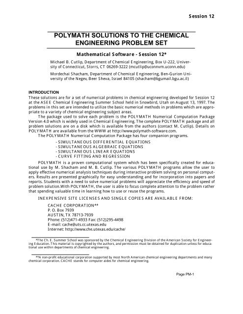
INTRODUCTION 

These solutions are for a set of numerical problems in chemical engineering developed for Session 12 

at the ASEE Chemical Engineering Summer School held in Snowbird, Utah on August 13, 1997. The 

problems in this set are intended to utilize the basic numerical methods in problems which are appropriate 

to a variety of chemical engineering subject areas. 

The package used to solve each problem is the POLYMATH Numerical Computation Package 

Version 4.0 which is widely used in Chemical Engineering. The complete POLYMATH package and all 

problem solutions are on a disk which is available from the authors (contact M. Cutlip). Details on 

POLYMATH are available from the WWW at http://www.polymath-software.com. 

The POLYMATH Numerical Computation Package has four companion programs. 

- SIMULTANEOUS DIFFERENTIAL EQUATIONS 

- SIMULTANEOUS ALGEBRAIC EQUATIONS 

- SIMULTANEOUS LINEAR EQUATIONS 

- CURVE FITTING AND REGRESSION 

POLYMATH is a proven computational system which has been specifically created for educational 

use by M. Shacham and M. B. Cutlip. The various POLYMATH programs allow the user to 

apply effective numerical analysis techniques during interactive problem solving on personal computers. 

Results are presented graphically for easy understanding and for incorporation into papers and 

reports. Students with a need to solve numerical problems will appreciate the efficiency and speed of 

problem solution.With POLYMATH, the user is able to focus complete attention to the problem rather 

that spending valuable time in learning how to use or reuse the programs. 

INEXPENSIVE SITE LICENSES AND SINGLE COPIES ARE AVAILABLE FROM: 

CACHE CORPORATION** 

P. O. Box 7939 

AUSTIN, TX 78713-7939 

Phone: (512)471-4933 Fax: (512)295-4498 

E-mail: cache@uts.cc.utexas.edu 

Internet: http://www.che.utexas.edu/cache/ 

*The Ch. E. Summer School was sponsored by the Chemical Engineering Division of the American Society for Engineering 

Education. This material is copyrighted by the authors, and permission must be obtained for duplication unless for educational 

use within departments of chemical engineering. 

**A non-profit educational corporation supported by most North American chemical engineering departments and many 

chemical corporation. CACHE stands for computer aides for chemical engineering. 

Page PM-1 

Session 12

Page PM-2 MATHEMATICAL SOFTWARE PACKAGES IN CHEMICAL ENGINEERING 

Polymath Problem 1 Solution 

Equation (1) can not be rearranged into a form where V can be explicitly expressed as a function of T 

and P. However, it can easily be solved numerically using techniques for nonlinear equations. In order 

to solve Equation (1) using the POLYMATH Simultaneous Algebraic Equation Solver, it must be 

rewritten in the form 

PM-(1) 

where the solution is obtained when the function is close to zero, f( V) 

≈ 

0 . Additional explicit equations 

and data can be entered into the POLYMATH program in direct algebraic form. The POLY- 

MATH program will reorder these equations as necessary in order to allow sequential calculation. 

The POLYMATH equation set for this problem are given by 

Equations: 

f(V)=(P+a/(V^2))*(V-b)-R*T 

P=56 

R=0.08206 

T=450 

Tc=405.5 

Pc=111.3 

Pr=P/Pc 

a=27*(R^2*Tc^2/Pc)/64 

b=R*Tc/(8*Pc) 

Z=P*V/(R*T) 

Search Range: 

V(min)=0.4, V(max)=1 

In order to solve a single nonlinear equation with POLYMATH, an interval for the expected solution 

variable,V in this case, must be entered into the program. This interval can usually be found by 

consideration of the physical nature of the problem. 

(a) For part (a) of this problem, the volume calculated from the ideal gas law as V = 0.66 liter/gmol 

can be a basis for specifying the required solution interval. An interval for the expected solution 

for V can be entered as between 0.4 as the lower limit and 1.0 as the higher limit. The POLYMATH 

solution, which is given in Figure PM-(1) for T = 450 K and P = 56 atm, yields V = 0.5749 liter/gmol 

where the compressibility factor is Z = 0.8718. 

(b) Solution for the additional pressure values can be accomplished by changing the equations 

in the POLYMATH program for P and Pr 

to 

Pr=1 

P=Pr*Pc 

a 

f( V) 

P 

V 2 

= ⎛ + 

⎝ 

------ ⎞( V – b) 

– RT 

⎠ 

Additionally, the bounds on the molar volume V may need to be altered to obtain an interval where 

there is a solution. Subsequent program execution for the various Pr’s 

is required. 

(c) The calculated molar volumes and compressibility factors are summarized in Table (1). 

These calculated results indicate that there is a minimum in the compressibility factor Z at approximately 

Pr 

= 2. The compressibility factor then starts to increase and reaches Z = 2.783 for Pr 

= 20 .

Polymath Problem 1 Solution Page PM-3 

f(V) 

Figure PM-1 Plot of f(V) versus V for van der Waals Equation 

Table PM-1 

P(atm) 

Compressibility Factor for Gaseous Ammonia at 450 K 

P 

r 

V Z 

56 0.503 .574892 0.871827 

111.3 1.0 .233509 0.703808 

222.6 2.0 .0772676 0.465777 

445.2 4.0 .0606543 0.731261 

1113.0 10.0 .0508753 1.53341 

2226.0 20.0 .046175 2.78348 

Variable Value f( ) 

V 0.574892 0 

P 56 

R 0.08206 

T 450 

Tc 405.5 

Pc 111.3 

Pr 0.503145 

a 4.19695 

b 0.03737712 

Z 0.871827

Page PM-4 

MATHEMATICAL SOFTWARE PACKAGES IN CHEMICAL ENGINEERING 


(a) The coefficients and the constants in the Equation Set Equation (6) can be directly introduced 

into the POLYMATH Linear Equation Solver in matrix form as shown 

The solution is 

Name x1 x2 x3 x4 b 

1 0.07 0.18 0.15 0.24 10.5 

2 0.04 0.24 0.1 0.65 17.5 

3 0.54 0.42 0.54 0.1 28 

4 0.35 0.16 0.21 0.01 14 

Variable Value 

which corresponds to the unknown flow rates of D1 

min, and B2 

= 17.5 mol/min. 

x1 26.25 

x2 17.5 

x3 8.75 

x4 17.5 

= 26.25 mol/min, B1 

= 17.5 mol/min, D2 

= 8.75 mol/ 

(b) The overall balances and individual component balances on column #2 given in Equation Set 

(7) can be solved algebraically to give XDx 

= 0.114, XDs 

= 0.120, XDt 

= 0.492 and XDb 

= 0.274. Similarly, 

overall balance and individual component balances on column #3 presented as Equation Set (8) yield 

XBx 

= 0.210, XBs 

= 0.4667, XBt 

= 0.2467 and XBb 

= 0.0767.



(a) Data Regression with a Polynomial The POLYMATH Polynomial, Multiple Linear and 

Nonlinear Regression Program can be used to solve this problem by first entering the data in a similar 

manner to using a spreadsheet. Let us denote the column of temperature data in °C as TC and the column 

of pressure data as P. 

This POLYMATH worksheet is reproduced in Figure PM-(2) where the 

first two columns are used in the polynomial regressions. 

Figure PM-2 POLYMATH Entry for Regressions 

A polynomial regression option within POLYMATH when the dependent variable column titled 

P is regressed with the independent variable TC corresponds directly to Equation (9). The results are 

summarized in Figure PM-(3) which also presents the value of the variance (var,) for each polynomial. 

The variance indicates that the polynomial which best represents the data in this case is the 4th 

degree. 

(b) Regression with Clausius-Clapeyron Equation Data regression with the Clausius-Clapeyron 

expression, Equation (10), can be accomplished by three additional transformed variables (columns) 

in the POLYMATH program used for part (a). Columns can be defined by the relationships: 

logP = log(P), TK= T + 273.15, and neginvTK = -1/TK as indicated in Figure PM-(2). A request for linear 

regression when the first (and only) independent variable column is neginvTK and the dependent 

variable column is logP yields the following plot and numerical results from POLYMATH as shown in 

Figure PM-(4). 

(c) Regression with the Antoine Equation This expression, Equation (11), cannot be linearized 

and so it must be regressed with nonlinear regression option of the POLYMATH Polynomial, Multiple 

Linear and Nonlinear Regression Program. 

With this option, the user must supply initial estimates. 

In this case, it is helpful to use the initial estimates for A and B which were determined in part (b) 

and use the estimate for C as 273.15. Direct entry of Equation (11) with the initial estimates gives the 

converged results shown in Figure PM-(5).

Page PM-6 


Figure PM-3 POLYMATH Results for Fitting Polynomials to Vapor Pressure Data 

Parameter Value 

0.95 Conf 

Interval 

A 8.75201 0.542335 

B 2035.33 153.628 

Var 0.00759156 

Figure PM-4 POLYMATH Results for Regression of Clausius-Clapeyron Equation


Figure PM-5 POLYMATH Results for Nonlinear Regression of Antoine Equation

Page PM-8 



The Equation Set (13) can be entered into the POLYMATH Simultaneous Algebraic Equation Solver, 

but the nonlinear equilibrium expressions must be written as functions which are equal to zero at the 

solution. A simple transformation of the equilibrium expressions of Equation Set Equation (12) to the 

required functional form yields 

PM-(2) 

The above equation set may be difficult to solve because the division by unknowns may make most 

solution algorithms diverge. 

Expediting the Solution of Nonlinear Equations 

An additional simple transformation of the nonlinear function can make many functions much less 

nonlinear and easier to solve by simply eliminating division by the unknowns. In this case, the Equation 

Set PM-(2) can be modified to 

PM-(3) 

The POLYMATH equation set utilizing Equation Set PM-(3) with the initial conditions for part 

(a) is given below. 

Equations: 

f(CD)=CC*CD-KC1*CA*CB 

f(CX)=CX*CY-KC2*CB*CC 

f(CZ)=CZ-KC3*CA*CX 

KC1=1.06 

CY=CX+CZ 

KC2=2.63 

KC3=5 

CA0=1.5 

CB0=1.5 

CC=CD-CY 

CA=CA0-CD-CZ 

CB=CB0-CD-CY 

Initial Estimates: 

CD(0)=0 

CX(0)=0 

CZ(0)=0 

f( CD) f( CX) f( CZ) CCC D 

= ---------------- – K 

C AC C1 

B 

CX CY = ---------------- – K 

CBC C2 

C 

CZ = ---------------- – K 

C AC C3 

X 

f( CD) = CCC D – K C1C ACB f( CX) = CX CY – K C2C BC C 

f( CZ) = 

CZ – K C3C AC X 

(a), (b) and (c) The POLYMATH solutions are summarized in Table PM-(2) for the three sets of 

initial conditions. Note that the initial conditions for problem part (a) converged to all positive concentrations. 

However the initial conditions for parts (b) and (c) converged to some negative values for 

some of the concentrations. Thus a “reality check” on Table PM-(2) for physical feasibility reveals that


the negative concentrations in parts (b) and (c) are the basis for rejecting these solutions as not representing 

a physically valid situation. 

Table PM-2 POLYMATH Solutions of the Chemical Equilibrium Problem 

Variable Part (a) Part (b) Part (c) 

C D 0.7053 0.05556 1.070 

C X 0.1778 0.5972 -0.3227 

C Z 0.3740 1.082 1.131 

C A 0.4207 0.3624 -0.7006 

C B 0.2429 -0.2348 -0.3779 

C C 0.1536 -1.624 0.2623 

C Y 0.5518 1.679 0.8078



(a) For conditions similar to those of this problem, the Reynolds number will not exceed 1000 so 

that only Equations (16) and (17) need to be applied. The logic which selects the proper equation 

based on the value of Re can be employed using the “if... then... else...” statement within the POLY- 

MATH Simultaneous Algebraic Equation Solver. 

CD = if ( Re < 0.1) 

then ( 24 ⁄ Re) 

else 24 1 0.14Re 0.7 

( × ( + ) ) 

PM-(4) 

Equation (13) should be rearranged in order to avoid possible division by zero and negative 

square roots as it is entered into the form of a nonlinear equation for POLYMATH. 

2 

f( vt) = vt ( 3CDρ ) – 4 g( ρ p – ρ)Dp 

The following equation set can be solved by POLYMATH. 

Equations: 

f(vt)=vt^2*(3*CD*rho)-4*g*(rhop-rho)*Dp 

g=9.80665 

rhop=1800 

rho=994.6 

Dp=0.208e-3 

vis=8.931e-4 

Re=Dp*vt*rho/vis 

CD=if (Re



Equations (20) to (22), together with the numerical data and initial values given in the problem 

statement, can be entered into the POLYMATH Simultaneous Differential Equation Solver. The initial 

startup is from a temperature of 20°C in all three tanks, thus this is the appropriate initial condition 

for each tank temperature. The final value or steady state value can be determined by solving the 

differential equations to steady state by giving a large time interval for the numerical solution. Alternately 

one could set the time derivatives to zero, and solve the resulting algebraic equations. In this 

case, it is easiest just to numerically solve the differential equations to large value of t where steady 

state is achieved. The POLYMATH coding for this problem is shown below. 

Equations: 

d(T1)/d(t)=(W*Cp*(T0-T1)+UA*(Tsteam-T1))/(M*Cp) 



W=100 

Cp=2.0 

T0=20 

UA=10. 

Tsteam=250 

M=1000 

Initial Conditions: 

t(0)=0 

T1(0)=20 

T2(0)=20 

T3(0)=20 

Final Value: 

t(f)=200 

The time to reach steady state is usually considered to be the time to reach 99% of the final 

steady state value for the variable which is increasing and responds the most slowly. For this problem, 

T 3 increases the most slowly, and the steady state value is found to be 51.317°C. In POLYMATH, this 

can be easily done by displaying the output in tabular form for T 1 , T 2 , and T 3 so that the approach to 

steady state can accurately be observed. Thus the time must be determined when T 3 reaches 

0.99(51.317) or 50.804 °C. Again the tabular form of the output is useful in determining this time as 

illustrated in Table 4 yielding the time to steady state as approximately 63.0 min. A plot of the three 

tank temperatures from POLYMATH is given in Figure PM-(6). 

Table PM-4 Tabular Output Option from POLYMATH 

t T3 

60 50.662233 

60.5 50.688128 

61 50.713042 

61.5 50.737011 

62 50.760068 

62.5 50.782246 

63 50.803577 

63.5 50.82409


Table PM-4 Tabular Output Option from POLYMATH 

t T3 

64 50.843817 

64.5 50.862784 

65 50.88102 

Figure PM-6 Dynamic Temperature Response in the Three 

Tanks



Solving Higher Order Ordinary Differential Equations 

Most mathematical software packages can solve only systems of first order ordinary differential equations 

(ODE’s). Fortunately, the solution of an n-th order ODE can be accomplished by expressing the 

equation by a series of simultaneous first order differential equations each with a boundary condition. 

This is the approach that is typically used for the integration of higher order ODE’s. 

(a) Equation (23) is a second order ODE, but it can be converted into a system of first order 

equations by substituting new variables for the higher order derivatives. In this particular case, a 

new variable y can be defined which represent the first derivation of C A with respect to z. Thus Equation 

(23) can be written as the equation set 

PM-(6) 

This set of first order ODE’s can be entered into the POLYMATH Simultaneous Differential 

Equation Solver for solution, but initial conditions for both C A and y are needed. Since the initial 

condition of y is not known, an iterative method (also referred to as a shooting method) can be used to 

find the correct initial value for y which will yield the boundary condition given by Equation (25). 

Shooting Method-Trial and Error 

The shooting method is used to achieve the solution of a boundary value problem to one of an iterative 

solution of an initial value problem. Known initial values are utilized while unknown initial values 

are optimized to achieve the corresponding boundary conditions. Either “trial and error” or variable 

optimization techniques are used to achieve convergence on the boundary conditions. 

For this problem, a first “trial and error” value for the initial condition of y, for example y 0 = -150, 

is used to carry out the integration and calculate the error for the boundary condition designated by ε. 

Thus the difference between the calculated and desired final value of y at z = L is given by 

PM-(7) 

Note that for this example, y f ,desired = 0 and thus ε(y 0 ) = y f,calc only because this desired boundary condition 

is zero. 

The equations as entered in the POLYMATH Simultaneous Differential Equation Solver for an 

initial “trial and error” solution are 

Equations: 

d(CA)/d(z)=y 

d(y)/d(z)=k*CA/DAB 

k=0.001 

DAB=1.2E-9 

err=y 


z(0)=0 

CA(0)=0.2 

y(0)=-150 

Final Value: 

z(f)=0.001 

dCA ----------- = y 

dz 

dy 

----dz 

= 

ε( y0) = 

yf, calc – 

k 

----------- C 

D A 

AB 

yf, desired 

The calculation of err in the POLYMATH equation set which corresponds to Equation PM-(7) is only


valid at the end of the ODE solution. Repeated reruns of this POLYMATH equation set with different 

initial conditions for y can be used in a “trial and error” mode to converge upon the desired boundary 

condition for y 0 where ε(y 0 ) or err ≅ 0. Some results are summarized in Table PM-(5) for various values 

Table PM-5 Trial Boundary Conditions for Equation Set (6) in Problem 7 Part (a) 

y 0 (z = 0) -120. -130. -140. -150. 

y f,calc (z = L) 17.23 2.764 -11.70 -26.16 

ε(y 0) 17.23 2.764 -11.70 -26.16 

of y0 . The desired initial value for y0 lies between -130 and -140. This “trial and error” approach can be 

continued to obtain a more accurate value for y0 , or an optimization technique can be applied. 

Newton’s Method for Boundary Condition Convergence 

A very useful method for optimizing the proper initial condition is to consider this determination 

to be a problem in finding the zero of a function. In the notation of this problem, the variable to be 

optimized is y0 and the objective function is ε(y0 ) which is defined by Equation PM-(7). 

Newton’s method, an effective method for optimizing a single variable, can be applied here to 

minimize the above objective function. According to this method, an improved estimate for y0 can be 

calculated using the equation 

y0, new = y0 – ε( y0) ⁄ ε'( y0) PM-(8) 

where ε'( y0) is the derivative of ε at y = y0. The derivative, ε'( y0) , can be estimated using a finite 

difference approximation 

ε( y0 + δ y0) – ε( y0) ε'( y0) ≅ ------------------------------------------------- 

PM-(9) 

δ y0 where δ y0 is a small increment in the value of y0 . It is very convenient that ε( y0 + δ y0) can be calculated 

simultaneously with the numerical ODE solution for ε( y0) thereby allowing calculation of ε'( y0) from Equation PM-(9) and a new estimate for y0 from Equation PM-(8). 

Using δ = 0.0001 for this example, the POLYMATH equation set for carrying out the first step in 

Newton’s method procedure is given by 

Equations: 

d(CA)/d(z)=y 

d(y)/d(z)=k*CA/DAB 

d(CA1)/d(z)=y1 

d(y1)/d(z)=k*CA1/DAB 

k=0.001 

DAB=1.2E-9 

err=y-0 

err1=y1-0 

y0=-130 

L=.001 

delta=0.0001 

CAanal=0.2*cosh(L*(k/DAB)^.5*(1-z/L))/(cosh(L*(k/DAB)^.5)) 

derr=(err1-err)/(.0001*y0) 

ynew=y0-err/derr 


z(0)=0


CA(0)=0.2 

y(0)=-130 

CA1(0)=0.2 

y1(0)=-130.013 

Final Value: 

z(f)=0.001 

This set of equations yields the results summarized in Table 6 where the new estimate for y 0 is 

the final value of the POLYMATH variable ynew or -131.911. Another iteration of Newton’s method 

can be obtained by starting with the new estimate and modifying the initial conditions for y and y1 

and the value of y0 in the POLYMATH equation set. The second iteration indicates that the err is 

approximately 3.e-4 and that ynew is unchanged indicating that convergence has been obtained. For 

the value of y0 = -131.911, the numerical and analytical solutions are equal to at least six significant 

digits. 

Table PM-6 Partial Results for Selected Variables during 1st Newton’s Method Iteration 

Variable Initial Value 

Maximum 

Value 

Minimum 

Value Final Value 

z 0 0.001 0 0.001 

y -130 2.76438 -130 2.76438 

CA 0.2 0.2 0.140428 0.140461 

err -130 2.76438 -130 2.76438 

y1 -130.013 2.74558 -130.013 2.74558 

CA1 0.2 0.2 0.140446 -0.142229 

err1 -130.013 2.74558 -130.013 2.74558 

derr 1 1.44642 1 1.44642 

ynew -5.22675e-11 -5.22675e-11 -131.911 -131.911



This problem requires the simultaneous solution of Equation (27) while the temperature is calculated 

from the bubble point considerations implicit in Equation (29). A system of equations comprising of 

differential and implicit algebraic equations is called “differential algebraic” or a DAE system. There 

are several numerical methods for solving DAE systems. Most problem solving software packages 

including POLYMATH do not have the specific capability for DAE systems. 

Approach 1 The first approach will be to use the controlled integration technique proposed by 

Shacham, et al. 4 . Using this method, the nonlinear Equation (29) is rewritten with an error term 

given by 

ε = 1 – k1x 1 – k2x 2 

PM-(10) 

where the ε calculated from this equation provides the basis for keeping the temperature of the distillation 

at the bubble point. This is accomplished by changing the temperature in proportion to the 

error in an analogous manner to a proportion controller action. Thus this can be represented by 

another differential equation 

dT 

--------- = K PM-(11) 

dx cε 2 

where a proper choice of the proportionality constant Kc will keep the error below a desired error tolerance. 

The calculation of Kc is a simple trial and error procedure for most problems. At the beginning Kc is set to a small value (say Kc = 1), and the system is integrated. If ε is too large, then Kc must be 

increased and the integration repeated. This trial and error procedure is continued until ε becomes 

smaller than a desired error tolerance throughout the entire integration interval. 

The temperature at the initial point is not specified in the problem, but it is necessary to start 

the problem solution at the bubble point of the initial mixture. This separate calculation can be carried 

out on Equation (29) for x1 = 0.6 and x2 = 0.4 and the Antoine equations using the POLYMATH 

Simultaneous Algebraic Equation Solver. The solution equation set is given by 

Equations: 

f(Tbp)=xA*PA+xB*PB-760*1.2 

xA=0.6 

PA=10^(6.90565-1211.033/(Tbp+220.79)) 

PB=10^(6.95464-1344.8/(219.482+Tbp)) 

xB=1-xA 

yA=xA*PA/(760*1.2) 

yB=xB*PB/(760*1.2) 

Search Range: 

Tbp(min)=60, Tbp(max)=120 

The resulting initial temperature is found to be T0 = 95.5851 . 

The system of equations for the batch distillation as they are introduced into the POLYMATH 

6 

Simultaneous Differential Equation Solver using K c = 

0.5×10 

are 

Equations: 

d(L)/d(x2)=L/(k2*x2-x2) 

d(T)/d(x2)=Kc*err 

Kc=0.5e6


k2=10^(6.95464-1344.8/(T+219.482))/(760*1.2) 

x1=1-x2 

k1=10^(6.90565-1211.033/(T+220.79))/(760*1.2) 

err=(1-k1*x1-k2*x2) 


x2(0)=0.4 

L(0)=100 

T(0)=95.5851 

Final Value: 

x2(f)=0.8 

and the partial results from the solution are summarized in Table PM-(7) 

Table PM-7 Partial Results for DAE Binary Distillation Problem 

Variable Initial Value Maximum Value Minimum Value Final Value 

x2 0.4 0.8 0.4 0.8 

L 100 100 14.0456 14.0456 

T 95.5851 108.569 95.5851 108.569 

k2 0.532535 0.785753 0.532535 0.785753 

Kc 500000 500000 500000 500000 

x1 0.6 0.6 0.2 0.2 

k1 1.31164 1.8566 1.31164 1.8566 

err -3.64587e-07 7.75023e-05 -3.64587e-07 7.75023e-05 

The final values from the table indicate that 14.05 mol of liquid remain in the column when the 

concentration of the toluene reaches 80%. During the distillation the temperature increases from 

– 7 

95.6 °C to 108.6 °C . The error calculated from Equation (10) increases from about – 3.6×10 

to 

– 5 

7.75×10 

during the numerical solution, but it is still small enough for the solution to be considered 

as accurate. 

Approach 2 A different approach for solving this problem can be used because Equation (29) 

can be differentiated with respect to x 2 to yield 

dT 

-------dx2 

( k2 – k1) – B1 

( 10) 

x1k1 ( C1 + T) 

2 

– B2 

------------------------ x2k2 ( C2 + T) 

2 

= 

-------------------------------------------------------------------------------------------------------ln 

+ ------------------------ 

PM-(12) 

Thus Equation PM-(12) can provide the bubble point temperature during the simultaneous integration 

with Equation (27). The equation set to be used with the POLYMATH Simultaneous Differential 

Equation Solver is given by 

Equations: 

d(L)/d(x2)=L/(k2*x2-x2) 

d(T)/d(x2)=(k2-k1)/(ln(10)*(x1*k1*(-1211.033)/(220.79+T)^2+x2*k2*(-1344.8)/ 

(219.482+T)^2))


k2=10^(6.95464-1344.8/(T+219.482))/(760*1.2) 

k1=10^(6.90565-1211.033/(T+220.79))/(760*1.2) 

x1=1-x2 


x2(0)=0.4 

L(0)=100 

T(0)=95.5851 

Final Value: 

x2(f)=0.8 

The POLYMATH solution to this problem is essentially the same as that found in Approach 1.



Introduction of the above equations including the numerical values of the parameter provided in the 

problem statement into the POLYMATH program yields 

Equations 

d(x)/d(W)=-rA/FA0 

d(T)/d(W)=(.8*(Ta-T)+rA*delH)/(CPA*FA0) 

d(y)/d(W)=-0.015*(1-.5*x)*(T/450)/(2*y) 

Ta=500 

delH=-40000 

CPA=40 

FA0=5 

k=.5*exp((41800/8.314)*(1/450-1/T)) 

CA=.271*(1-x)*(450/T)/(1-.5*x)*y 

CC=.271*.5*x*(450/T)/(1-.5*x)*y 

Kc=25000*exp(delH/8.314*(1/450-1/T)) 

rA=-k*(CA^2-CC/Kc) 


W(0)=0 

x(0)=0 

T(0)=450 

y(0)=1 

W(f)=20 

(a) The requested plot for part (a) is shown in Figure PM-(7) where there is a rapid increase in 

conversion and temperature within the reactor at approximately the midpoint of the catalyst bed. The 

bed pressure drop is enhanced by the increased temperature and reduced pressure even though the 

number of moles is decreasing. 

×10 -3 

Figure PM-7 Conversion, Reduced Pressure, and Temperature Profiles in Catalytic Reactor 

(b) This rapid increase is due to the exothermic reaction rapidly accelerating due to the increasing 

temperature even though the reactant concentration falling. Equilibrium is rapidly achieved after 

this hot spot is achieved with the temperature and conversion only reducing slightly due to the exter-


nal heat transfer which tends to slightly cool the reactor as the reacting mixture continues toward the 

reactor exit. 

(c) The concentration profiles shown in Figure PM-(8) reflect the net effects of reaction rate and 

changes in temperature and pressure within the reactor. 

Figure PM-8 Concentration Profiles in Catalytic Reactor



This problem requires the solution of Equations (40) and (42) through (47) which can be accomplished 

with the POLYMATH Simultaneous Differential Equation Solver. The step change in the inlet temperature 

can be introduced at t = 10 by using the POLYMATH “if... then... else...” statement to provide 

the logic for a variable to change at a particular value of t. The generation of a step change at t = 10, 

for example, is accomplished by the POLYMATH program statement 

step=if (t


Figure PM-9 Open Loop Response to Step Down in Inlet Feed Temperature at t = 10 min 

later) with more error at the initiation of the step change. This verifies that the Padé approximation 

for dead time is providing the one minute time delay. 

(b) Closed Loop Performance The closed loop performance of the PI controller requires the 

change of K c from zero in part (a) to the baseline proportional gain of 50. This simple change results in 

the temperature transients shown in Figure PM-(10). 

(c) Closed Loop Performance for K c = 500 The increase of a factor of 10 in the proportional gain 

from the baseline case gives the unstable result plotted in Figure PM-(11). This is clearly an undesirable 

result.


Figure PM-10 Closed Loop Response to Step Down in Inlet Feed Temperature at t = 10 min. 

Figure PM-11 Closed Loop Response to Step Down in Inlet Feed Temperature at t = 10 min for K c = 500.


(d) Closed Loop Performance for Only Proportional Control The removal of the integral control 

action gives the stable result plotted in Figure PM-(12). Note that there is offset from the set point 

Figure PM-12 Closed Loop Response for only Proportional Control. 

when the system returns to steady state operation. This is always the case for only proportional control, 

and the use of integral control allows the offset to be eliminated.


(e) Closed Loop Performance with Limits on q There are many times in control when limits 

must be established. In this example, the limits on q can be achieved by a POLYMATH “if... then... 

else...” statement which can be utilized as shown below 

qlim=if(q=2.6*10000)then(2.6*10000)else (q)) 

The complete POLYMATH equation set for part (e) of this problem is 

Equations: 

d(T)/d(t)=(WC*(Ti-T)+qlim)/rhoVCp 

d(T0)/d(t)=(T-T0-(taud/2)*dTdt)*2/taud 

d(Tm)/d(t)=(T0-Tm)/taum 

d(errsum)/d(t)=Tr-Tm 

WC=500 

Ti=60 

rhoVCp=4000 

taud=1 

taum=5 

Kc=5000 

tauI=2 

step=if (t


Figure PM-13 Closed Loop Response for only Proportional 

Control. 

Figure PM-14 Closed Loop Response for only Proportional 

Control.

Page PM-27 MATHEMATICAL SOFTWARE PACKAGES IN CHEMICAL ENGINEERING

Page PM-28 MATHEMATICAL SOFTWARE PACKAGES IN CHEMICAL ENGINEERING

polymath solutions to the chemical engineering problem set

Create successful ePaper yourself

Delete template?

Save as template?