manuscript - KTH Mechanics
manuscript - KTH Mechanics
manuscript - KTH Mechanics

You also want an ePaper? Increase the reach of your titles
YUMPU automatically turns print PDFs into web optimized ePapers that Google loves.
École Polytechnique<br />
Laboratoire d’Hydrodynamique<br />
Thèse présentée pour obtenir le grade de<br />
DOCTEUR DE L’ÉCOLE POLYTECHNIQUE<br />
Spécialité : Mécanique<br />
par<br />
Pierre AUGIER<br />
Turbulence en milieu stratifié,<br />
étude des mécanismes de la cascade<br />
Soutenue le 21 octobre 2011 devant un jury composé de<br />
Paul BILLANT directeur de thèse LadHyX, Palaiseau<br />
Jean-Marc CHOMAZ directeur de thèse LadHyX, Palaiseau<br />
Thierry DAUXOIS examinateur ENS Lyon, Lyon<br />
Olivier Eiff examinateur IMFT, Toulouse<br />
Bach Lien HUA examinatrice IFREMER, Plouzané<br />
Erik LINDBORG rapporteur <strong>KTH</strong>, Stockholm, Suède<br />
Frédéric MOISY rapporteur FAST, Orsay<br />
Joël SOMMERIA examinateur LEGI, Grenoble
© Pierre Augier, septembre 2011<br />
Edité par : Ecole Polytechnique<br />
LadHyX<br />
Ecole Polytechnique<br />
FRANCE
Résumé<br />
La turbulence fortement influencée par une stratification stable en densité est étudiée<br />
expérimentalement, numériquement et théoriquement. Ce type de turbulence est rencontré<br />
dans l’atmosphère et les océans dans une gamme d’échelles intermédiaires où<br />
la force de Coriolis est négligeable.<br />
Dans une première partie, la transition à la turbulence d’un écoulement simple :<br />
une paire de tourbillons colonnaires contra-rotatifs est étudiée. Des Simulations Numériques<br />
Directes (DNS) montrent que lorsque la dissipation est suffisamment faible,<br />
deux instabilités secondaires, de cisaillement et gravitationnelle, se développent après<br />
l’instabilité zigzag. La taille caractéristique des tourbillons de Kelvin-Helmholtz est<br />
de l’ordre de l’échelle de flottabilité. Ces deux instabilités mènent à une transition à<br />
la turbulence qui présente des spectres anisotropes similaires à ceux associés à la turbulence<br />
stratifiée pleinement développée. Pour la première fois, un retour à l’isotropie<br />
est observé pour des échelles inférieures à l’échelle d’Ozmidov.<br />
Dans une deuxième partie, un écoulement pleinement turbulent forcé par plusieurs<br />
générateurs de dipoles est étudié. Les expériences aux plus grands nombres de Reynolds<br />
de flottabilité ont permis pour la première fois de quasiment atteindre le régime<br />
de turbulence fortement stratifié. Les simulations numériques forcées dans l’espace<br />
physique avec le même type de forcage ont permis de reproduire les résultats expérimentaux<br />
et de les étendre aux grands nombres de Reynolds de flottabilité. Elles<br />
révèlent que la plus grande échelle des retournements est de l’ordre de l’échelle de<br />
flottabilité. Enfin, une généralisation de la loi des 4/5 de Kolmogorov est proposée<br />
pour la turbulence stratifiée.<br />
Abstract<br />
Turbulence strongly influenced by a stable density stratification is studied experimentally,<br />
numerically and theoretically. This type of turbulence is encountered in the<br />
atmosphere and Oceans in an intermediate range of scales for which the Coriolis force<br />
is negligible.<br />
In a first part, the transition to turbulence of a simple flow: a pair of columnar<br />
contra-rotating vortices is studied. Direct Numerical Simulations (DNS) show<br />
that when the dissipation is sufficiently weak, two secondary instabilities, the shear<br />
and gravitational instabilities, develop after the zigzag instability. The characteristic<br />
length scale of the Kelvin-Helmholtz billows is of the order of the buoyancy scale.<br />
Both instabilities lead to a transition to turbulence which exhibits anisotropic spectra<br />
similar to those associated to fully developed strongly stratified turbulence. For the<br />
first time, a return to isotropy is observed for scales smaller than the Ozmidov length<br />
scale.<br />
In a second part, a fully developed turbulent flow forced with several vortex generators<br />
is studied. The experiments at the larger buoyancy Reynolds numbers have<br />
enabled for the first time to nearly reach the strongly stratified turbulent regime.<br />
These experimental results have been reproduced and extended to larger Reynolds<br />
numbers with numerical simulations forced in physical space with the same type of<br />
forcing. They reveal that the larger scale of the overturnings is of the order of the<br />
buoyancy scale. Finally, a generalisation of the 4/5s Kolmogorov law is proposed for<br />
stratified turbulence.<br />
iii
iv<br />
Remerciements<br />
Alors que j’écris ces lignes, ce manuscrit de thèse est bouclé et je suis à Waikiki,<br />
Honolulu, Hawaii ! Dans le cadre de mon post-doc au <strong>KTH</strong> à Stockholm, nous allons<br />
commencer une collaboration sur la dynamique de l’atmosphère avec des chercheurs<br />
hawaïens et japonais. Cette thèse est bien finie : passons au remerciements !<br />
Cette thèse est le fruit du travail collectif qui a duré trois ans. En première ligne,<br />
il y avait bien sûr mes directeurs de thèse et moi. Mais pour le reste tout est affaire<br />
d’environnement général.<br />
Les résultats de cette thèse sont pour moi de deux natures. Il y a bien sûr les résultats<br />
et des productions scientifiques. Mais ce travail a aussi fait de moi un “docteur”,<br />
jeune scientifique capable (paraît-il) d’une activité propre de recherche et d’enseignement.<br />
Ces remerciements ont donc une connotation personnelle particulière et viennent<br />
du fond du coeur. Je suis sincèrement très reconnaissant envers tous ceux qui m’ont<br />
permis de bien vivre la période passionnante et éminemment formatrice qu’a été cette<br />
thèse.<br />
Merci d’abord à mes deux directeurs de thèse si complémentaires. Merci de m’avoir<br />
laissé tant de liberté et d’avoir été en même temps disponibles et toujours intéressés.<br />
Merci Paul ! Merci de m’avoir appris tant de choses, autant en terme de connaissances<br />
hydrodynamiques et techniques qu’en terme d’attitude scientifique : rigueur,<br />
honnêteté, persévérance, perfectionnisme... Merci aussi d’avoir été toujours prêt à réfléchir<br />
et aider à avancer. Merci pour cet extraordinaire travail sur la rédaction des<br />
articles. Si un jour j’arrive à écrire indépendamment un article, ce sera beaucoup grâce<br />
à toi !<br />
Merci Jean-Marc ! Merci pour ces discussions scientifiques et non-scientifiques toujours<br />
si enrichissantes surtout quand on arrive à suivre. Merci de montrer qu’on peut<br />
continuer à faire de la recherche activement tout en étant directeur du labo, rameur,<br />
artiste scientifique et cavalier malchanceux luttant contre les tracteurs.<br />
Je dois des remerciements spéciaux à Axel Deloncle pour le code ns3d si efficace<br />
et si bien commenté ; à Sébastien Galtier pour cette expérience de collaboration avec<br />
un chercheur travaillant dans un domaine voisin ; et à Maria Eletta Negretti pour son<br />
aide précieuse sur l’expérience et la PIV, mais bien plus généralement pour sa présence<br />
qui m’a permis de bien commencer cette thèse.<br />
Merci à mes deux rapporteurs de thèse, Erik Lindborg et Frédéric Moizy d’avoir lu<br />
de façon critique et constructive ce long manuscrit. Vos remarques pertinentes m’ont<br />
été très précieuses. Merci à mes examinateurs de thèse d’être venu à Paris depuis<br />
Brest, Grenoble, Lyon et Toulouse pour participer à ma soutenance et apporter leurs<br />
regards sur mon travail.<br />
Cette thèse est aussi le résultat de l’unité de production scientifique du LadHyX,<br />
laboratoire de l’Ecole Polytechnique. Alors en plus de remercier ses directeurs (et<br />
directeur exécutif) en exercice pendant ma thèse, Patrick Huerre, Jean-Marc Chomaz<br />
et Christophe Clanet, je remercie tous ceux qui contribuent à la bonne marche de ce<br />
labo et à la bonne ambiance qui y règne.
Un merci tout particulier à Antoine Garcia et Daniel Guy de faire en sorte que les<br />
choses expérimentales et numériques fonctionnent et de donner de si bons conseils et<br />
si bonnes idées. Merci à Thérèse Lescuyer et aux autres secrétaires sans qui rien ne<br />
fonctionnerait ! Merci à mes compagnons de thèse, les autres thésards du labo. Je cède<br />
à la facilité de ne citer personne mais merci pour les bons moments, les discussions, le<br />
café, le foot et les coups de mains pour le numérique.<br />
Bon, comme une thèse ça vient de loin, merci maman, pour tout mais surtout<br />
d’avoir fait en sorte que je ne sois pas complètement largué en cours... Merci pour<br />
tout à toute la petite famille à qui je dois tant. Merci à mes instits et professeurs,<br />
surtout les sympas ! Merci au collège Fabre d’Eglantine, à l’Université de La Rochelle<br />
et à l’ENS Lyon. En fait, ce sera plus cours et plus complet de remercier carrément<br />
les services publics de notre République.<br />
Une thèse, c’est aussi une sacret bataille pendant laquelle il vaut mieux ne pas<br />
perdre courage au premier coup de vent. Merci aux amis, aux copains et à tous les<br />
gentils.<br />
Une thèse c’est une réflexion profonde et de longue haleine. En cela, détours et<br />
pauses ont pour moi été indispensables. Salut à la nature si belle et toujours étonnante.<br />
Salut à la culture humaine aussi. Merci aux artistes, philosophes et autres penseurs<br />
qui nous permettent de réfléchir hors de la doxa dominante et de tenter de vivre en<br />
homme libre.<br />
Pendant cette thèse, il y a eu matière à réfléchir sur les instabilités, les non-linéarités<br />
et la turbulence aussi ailleurs que dans les livres ! Le temps des crises et des bouleversements<br />
est revenu. Je voudrais saluer l’humanité impliquée dans cette grande aventure<br />
et tout particulièrement ceux qui en montrant tant de courage pour faire avancer l’intérêt<br />
général, m’en ont donné du courage ! Pendant cette thèse, des peuples ont pu<br />
faire tomber des tyrans ! Cela me conforte dans l’idée qu’il n’y a pas de raisons que<br />
l’on ne puisse pas vivre dignement tous. Je salue tous ceux qui se battent pour faire<br />
naître un autre monde où l’humain d’abord primera.<br />
En parlant de naissance, la fin de rédaction d’une thèse a quelque chose à voir<br />
avec un accouchement. Je salue Max qui a à peu près le même âge que ce manuscrit<br />
de thèse et ses parents qui doivent maintenant pouvoir commencer à dormir toute la<br />
nuit. Le long cheminement vers le progrès humain est assurément très tortueux mais<br />
j’ai la conviction qu’à ton échelle Max, il se remettra en marche. J’aime penser que<br />
cette thèse puisse, très modestement, s’inscrire dans ce mouvement.<br />
Pour finir en beauté, un très grand merci à mon amour, Marianne.<br />
Hawaï, le 4 décembre 2011.<br />
v
vi<br />
Foreword<br />
This <strong>manuscript</strong> thesis presents a work performed at the LadHyX, the hydrodynamics<br />
laboratory of Ecole Polytechnique. During 3 years, between September 2008 and<br />
August 2011, I have worked as a PhD student on the direction of Paul Billant and<br />
Jean-Marc Chomaz on the dynamics of the turbulence influenced by a stable density<br />
stratification.<br />
The major part of this <strong>manuscript</strong> is written in English. However, the first chapter<br />
presenting our motivations and a general introduction on the dynamics of fluids<br />
influenced by a stable density stratification and rotation is written in French. No-<br />
French-speaking readers and advanced readers can skip these basic reminders and go<br />
directly toward page 37 to begin with the main introduction on stratified turbulence.
Table des matières<br />
Summary . . . . . . . . . . . . . . . . . . . . . . . . . . . . . . . . . . iii<br />
Remerciements . . . . . . . . . . . . . . . . . . . . . . . . . . . . . . . iv<br />
Foreword . . . . . . . . . . . . . . . . . . . . . . . . . . . . . . . . . . vi<br />
Table des matières vii<br />
1 Introduction générale sur la dynamique des fluides géophysiques 1<br />
1.1 Contexte et motivations . . . . . . . . . . . . . . . . . . . . . . . . . . 1<br />
1.1.1 Notions de turbulence et de stratification . . . . . . . . . . . . 1<br />
1.1.2 Survol de la dynamique des enveloppes fluides terrestres . . . . 3<br />
1.2 Modèle : fluide incompressible newtonien stratifié en densité . . . . . . 11<br />
1.2.1 Approximation de Boussinesq . . . . . . . . . . . . . . . . . . . 11<br />
1.2.2 Formulation dans l’espace spectral . . . . . . . . . . . . . . . . 13<br />
1.3 Turbulence dans les fluides non-stratifiés, 3D et 2D . . . . . . . . . . . 16<br />
1.3.1 Turbulence 3D . . . . . . . . . . . . . . . . . . . . . . . . . . . 16<br />
1.3.2 Turbulence 2D . . . . . . . . . . . . . . . . . . . . . . . . . . . 22<br />
1.4 Eléments sur la dynamique des écoulements en milieu stratifié tournant 24<br />
1.4.1 Quantités conservées : énergie et enstrophie potentielle . . . . . 24<br />
1.4.2 Quelle échelle verticale ? Compétition rotation-stratification . . 26<br />
1.4.3 Turbulence quasi-géostrophique . . . . . . . . . . . . . . . . . . 29<br />
1.4.4 Ondes internes de gravité . . . . . . . . . . . . . . . . . . . . . 31<br />
2 Introduction on turbulence in stratified fluids 37<br />
2.1 Notion of turbulence in stratified fluids . . . . . . . . . . . . . . . . . . 38<br />
2.2 Dominant balance and buoyancy Reynolds number R . . . . . . . . . 41<br />
2.3 “Lilly’s stratified turbulence”, a brief historical review . . . . . . . . . 43<br />
2.4 The dynamics in the limit Fh ≪ 1, Fv ≪ 1 leads to Fv ∼ 1 . . . . . . 46<br />
2.5 Data analysis support the forward energy cascade hypothesis . . . . . 51<br />
2.6 Dynamics in the limit Fh ≪ 1, R ≫ 1 ⇒ Fv ∼ 1 . . . . . . . . . . . . 53<br />
2.7 Scientific issues and objectives . . . . . . . . . . . . . . . . . . . . . . . 58<br />
vii
viii TABLE DES MATIÈRES<br />
3 About the secondary instabilities on the zigzag instability 59<br />
3.1 Onset of secondary instabilities . . . . . . . . . . . . . . . . . . . . . . 59<br />
3.1.1 Introduction . . . . . . . . . . . . . . . . . . . . . . . . . . . . 61<br />
3.1.2 Numerical method and initial conditions . . . . . . . . . . . . . 62<br />
3.1.3 Description to the transition to small scales . . . . . . . . . . . 64<br />
3.1.4 Flow regimes in the parameter space [Re, Fh] . . . . . . . . . . 67<br />
3.1.5 Conclusion . . . . . . . . . . . . . . . . . . . . . . . . . . . . . 72<br />
3.2 Spectral analysis of the transition to turbulence . . . . . . . . . . . . . 73<br />
3.2.1 Introduction . . . . . . . . . . . . . . . . . . . . . . . . . . . . 75<br />
3.2.2 Methods . . . . . . . . . . . . . . . . . . . . . . . . . . . . . . . 77<br />
3.2.3 Global description of a simulation with Fh = 0.09 . . . . . . . . 79<br />
3.2.4 Variation of Fh and R . . . . . . . . . . . . . . . . . . . . . . . 84<br />
3.2.5 Effect of the Reynolds number and of the resolution for Fh = 0.09 89<br />
3.2.6 Decomposition of the horizontal fluxes for Fh = 0.09 . . . . . . 91<br />
3.2.7 Summary and conclusions . . . . . . . . . . . . . . . . . . . . . 94<br />
4 Studies of stratified turbulence forced with columnar dipoles 97<br />
4.1 Experimental study of a forced stratified turbulent-like flow . . . . . . 97<br />
4.1.1 Introduction . . . . . . . . . . . . . . . . . . . . . . . . . . . . 99<br />
4.1.2 Experimental design . . . . . . . . . . . . . . . . . . . . . . . . 102<br />
4.1.3 Description of the statistically stationary stratified flows . . . . 108<br />
4.1.4 Summary and conclusions . . . . . . . . . . . . . . . . . . . . . 120<br />
4.2 Numerical study of strongly stratified turbulence . . . . . . . . . . . . 123<br />
4.2.1 Introduction . . . . . . . . . . . . . . . . . . . . . . . . . . . . 126<br />
4.2.2 Numerical methodology . . . . . . . . . . . . . . . . . . . . . . 128<br />
4.2.3 Numerical forcing similar to the experimental one . . . . . . . 134<br />
4.2.4 Forcing with a randomly moving dipole generator . . . . . . . . 150<br />
4.2.5 Summary and conclusions . . . . . . . . . . . . . . . . . . . . . 161<br />
4.2.6 Appendix 1: mechanisms of vertical decorrelation . . . . . . . . 164<br />
4.2.7 Appendix 2: shear modes . . . . . . . . . . . . . . . . . . . . . 173<br />
5 Kolmogorov laws for stratified turbulence 177<br />
5.1 Introduction . . . . . . . . . . . . . . . . . . . . . . . . . . . . . . . . . 179<br />
5.2 Exact relation for the vectorial third-order structure function . . . . . 181<br />
5.2.1 Governing equations . . . . . . . . . . . . . . . . . . . . . . . . 181<br />
5.2.2 Stationary developed turbulence . . . . . . . . . . . . . . . . . 182<br />
5.2.3 von Kármán-Howarth equation . . . . . . . . . . . . . . . . . . 183<br />
5.2.4 Relation between T (r) and the energy flux . . . . . . . . . . . 184<br />
5.2.5 Exact result for homogeneous stratified turbulence . . . . . . . 184<br />
5.2.6 Weak stratification limit . . . . . . . . . . . . . . . . . . . . . . 185<br />
5.3 Kolmogorov law for anisotropic axisymmetric turbulence . . . . . . . . 185<br />
5.3.1 Assumption on the direction of the flux J . . . . . . . . . . . . 185<br />
5.3.2 Integration of ∇ · J = −4ε . . . . . . . . . . . . . . . . . . . . . 187<br />
5.3.3 Anisotropy in strongly stratified turbulence . . . . . . . . . . . 188<br />
5.3.4 Discussion on the appropriate value of n for stratified turbulence 190
TABLE DES MATIÈRES ix<br />
5.4 Conclusion . . . . . . . . . . . . . . . . . . . . . . . . . . . . . . . . . 191<br />
5.5 Appendix: alternative integration methods . . . . . . . . . . . . . . . 191<br />
5.5.1 Local integration . . . . . . . . . . . . . . . . . . . . . . . . . . 192<br />
5.5.2 Global integration on a surface . . . . . . . . . . . . . . . . . . 192<br />
6 Conclusions and Perspectives 195<br />
6.1 Conclusions . . . . . . . . . . . . . . . . . . . . . . . . . . . . . . . . . 195<br />
6.2 Suggestions for future work . . . . . . . . . . . . . . . . . . . . . . . . 197<br />
6.2.1 Large scale experiments . . . . . . . . . . . . . . . . . . . . . . 197<br />
6.2.2 Numerical and theoretical work . . . . . . . . . . . . . . . . . . 198<br />
6.2.3 Application to the study of geophysical fluids . . . . . . . . . . 200<br />
A Statistical and numerical methods 201<br />
A.1 Statistical description of stratified flows . . . . . . . . . . . . . . . . . 201<br />
A.1.1 Analyzing and projecting a turbulent flow state . . . . . . . . . 201<br />
A.1.2 Energy distribution (order 2 quantities) . . . . . . . . . . . . . 202<br />
A.1.3 Phase-dependent quantities and stability . . . . . . . . . . . . . 205<br />
A.1.4 Non-linear transfers, dissipation and buoyancy flux . . . . . . . 205<br />
A.2 Evolutions of the numerical code NS3D . . . . . . . . . . . . . . . . . 207<br />
A.2.1 NS3D: a parallel Navier-Stokes solver . . . . . . . . . . . . . . 207<br />
A.2.2 Time stepping and human interface . . . . . . . . . . . . . . . 208<br />
A.2.3 Outputs . . . . . . . . . . . . . . . . . . . . . . . . . . . . . . . 209<br />
A.2.4 Isotropic hyperviscosity . . . . . . . . . . . . . . . . . . . . . . 209<br />
A.2.5 Modified projectors . . . . . . . . . . . . . . . . . . . . . . . . . 210<br />
A.2.6 Forcing with coherent structures . . . . . . . . . . . . . . . . . 210<br />
B Tourbillons et dipôles colonnaires en milieu stratifié 211<br />
Bibliography 215
Chapitre 1<br />
Introduction générale sur la<br />
dynamique des fluides géophysiques<br />
1.1 Contexte et motivations<br />
Ce travail de thèse traite de la dynamique des écoulements turbulents fortement influencés<br />
par une stratification stable en densité. Nous abordons cette problématique<br />
sous l’angle de la dynamique des structures cohérentes et des instabilités hydrodynamiques.<br />
Dans ce chapitre, on commence par introduire les notions de turbulence et de<br />
stratification. Puis, on présente quelques éléments sur la dynamique des océans et de<br />
l’atmosphère qui est le principal domaine d’application des études de la turbulence en<br />
milieu stratifié.<br />
1.1.1 Notions de turbulence et de stratification<br />
Turbulence, cascade et mécanismes. La turbulence désigne dans le sens commun<br />
une agitation désordonnée. Dans le cadre de ce travail de recherche en hydrodynamique,<br />
le mot turbulence peut désigner différents régimes d’écoulements d’un fluide,<br />
modifiés ou non par la présence d’éléments influençant la dynamique (dimension de<br />
l’espace, stratification, rotation du référentiel, etc.). Ces écoulements partagent la caractéristique<br />
d’être fortement désordonnés, dans le sens qu’ils sont imprévisibles aux<br />
temps longs (chaotiques, avec une forte sensibilité aux conditions initiales) et présentent<br />
une superposition d’échelles spatiales et temporelles très différentes : de très<br />
grands et très petits tourbillons se côtoient. Par exemple, dans l’atmosphère, l’écoulement<br />
est forcé à une échelle de plusieurs centaines de kilomètres et la dissipation<br />
se produit à des échelles de quelques centimètres. Les grandes structures sont beaucoup<br />
trop grandes et trop rapides pour être influencées par la dissipation visqueuse.<br />
On quantifie cette influence par un nombre sans dimension, le nombre de Reynolds<br />
Re = ULh/ν, où U et Lh sont respectivement une vitesse et une taille horizontale<br />
caractéristiques et ν est la viscosité cinématique. Lorsque le nombre de Reynolds est<br />
suffisamment grand, les structures hydrodynamiques forcées évoluent selon leur propre<br />
dynamique non-linéaire sur des temps longs et des mécanismes non-linéaires liés à des<br />
1
2 CHAPITRE 1. INTRODUCTION GÉNÉRALE<br />
instabilités peuvent transférer de l’énergie vers des échelles différentes (plus petites<br />
dans le cas de la turbulence homogène et isotrope, dite classique). Ce processus se<br />
reproduit d’échelles en échelles avec une certaine invariance, ce qui mène à une répartition<br />
en énergie dans le domaine inertiel (aux échelles de la cascade) de type<br />
auto-similaire, avec des spectres en loi de puissance (par exemple en k −5/3 dans le<br />
cas de la turbulence classique, où k est le vecteur d’onde). Cette cascade d’énergie,<br />
décrite pour la première fois par Richardson (Frisch, 1995), permet dans certains cas<br />
(et en particulier dans le cas de la turbulence classique) le transfert de l’énergie vers les<br />
petites échelles dissipatives. Si cette représentation peut paraître relativement simple,<br />
elle décrit suffisamment bien la turbulence classique pour être à la base de raisonnements<br />
d’une grande puissance prédictive (cf. les lois de Kolmogorov rappelées dans<br />
la section 1.3). Précisons que les caractéristiques de la cascade turbulente classique<br />
ne dépendent pas (en fait peu) de la forme précise du forçage : cette cascade est dite<br />
“universelle”. Comment les processus turbulents sont-ils affectés par une stratification<br />
stable en densité ? Telle est la problématique traitée dans ce manuscrit de thèse.<br />
Stratification stable en densité. A chaque état d’un fluide caractérisé par des<br />
hétérogénéités de masse volumique 1 , on associe une énergie potentielle liée à la gravité.<br />
L’exemple du verre d’eau dans lequel on verse un peu de sirop est parlant. La<br />
dynamique tend vers l’état de moindre énergie potentielle : le sirop plus dense descend.<br />
Lorsque toute l’énergie cinétique aura été dissipée, le système se sera réorganisé<br />
de telle façon que le fluide le plus dense soit sous le fluide le moins dense avec des<br />
surfaces isodensités horizontales. Cet état stationnaire stratifié en densité est dynamiquement<br />
stable et donc très courant dans la nature. Dans ce travail de thèse, on<br />
étudie la dynamique des fluides autour de cet état de moindre énergie.<br />
Par contre cet état n’est pas stable thermodynamiquement. La diffusion du facteur<br />
de variation de la densité (la concentration d’un composant chimique ou la température)<br />
mènera à terme à l’homogénéisation de la densité. Mais la diffusion est très<br />
inefficace pour mélanger sur des grandes distances. On observe déjà ce phénomène<br />
d’inefficacité de la diffusion avec l’exemple du sirop dans un verre et cela est pire<br />
dans le cas de milieux beaucoup plus grands comme les fluides géophysiques (atmosphère,<br />
océans, mers, lacs). Ainsi la diffusion moléculaire de la stratification globale<br />
est négligeable dans les milieux fluides de grandes tailles qui sont très couramment<br />
stratifiés en densité. Notons que les hétérogénéités de densité proviennent de forçages<br />
thermodynamiques, souvent thermiques et la plupart du temps liés au soleil.<br />
Dans beaucoup de cas, la dynamique du fluide et la stratification en densité sont<br />
fortement couplées. La stratification intervient dans les équations sous la forme d’une<br />
pulsation, dite fréquence de Brunt-Väisälä N. On peut quantifier le couplage avec<br />
la dynamique fluide en comparant cette fréquence à la fréquence caractéristique du<br />
mouvement U/Lh. Lorsque la fréquence N est grande devant la fréquence caractéristique<br />
de l’écoulement, le ratio Fh = U/(NLh), nombre sans dimension appelé nombre<br />
de Froude horizontal, est petit et la stratification influence fortement l’écoulement.<br />
1 Comme en anglais, on dira de façon équivalente masse volumique et densité, sans faire de diffé-<br />
rence entre les deux notions.
1.1. CONTEXTE ET MOTIVATIONS 3<br />
L’expression du nombre de Froude montre que la stratification influence plus des<br />
écoulements de grande taille et relativement lents.<br />
Ainsi le principal domaine d’application de la turbulence fortement influencée par<br />
une stratification en densité est la dynamique des fluides géophysiques et astrophysiques.<br />
Pour être complet, mentionnons tout de même quelques autres applications<br />
plus technologiques. Les sillages des bateaux et des sous-marins constituent des écoulements<br />
influencés par la stratification de l’océan. La dynamique du mélange de fluides<br />
dans des grandes cuves industrielles (dans des contextes agroalimentaires, chimiques<br />
et pétrochimiques) peut également être turbulente et influencée par la stratification.<br />
1.1.2 Survol de la dynamique des enveloppes fluides terrestres<br />
L’enveloppe fluide terrestre constituée de l’atmosphère, des océans, des mers et des lacs<br />
est un système couplé d’une grande complexité dans lequel on observe une très grande<br />
diversité de phénomènes (voir par exemple les livres Pedlosky, 1987; Cushman-Roisin,<br />
1994; Vallis, 2006, traitant uniquement des aspects hydrodynamiques). Ses sous-parties<br />
aérienne et marines ont des différences fondamentales. Par exemple, les océans sont<br />
bornés par des parois latérales alors que l’atmosphère est fortement influencée par des<br />
effets liés à la compressibilité, à l’humidité et aux changements de phases, avec les<br />
nuages.<br />
L’étude d’un tel système met en jeu différentes approches scientifiques avec bien<br />
sûr en premier lieu l’observation, les mesures in-situ, base de l’océanographie et de<br />
la météorologie. L’interprétation des données et la compréhension du système global<br />
progressent grâce à une méthode classique de va-et-vient entre l’analyse et la synthèse.<br />
Le système complexe est d’abord décomposé en éléments relativement simples qui<br />
sont étudiés séparément (l’analyse). Puis le système est reconstruit de manière plus<br />
ou moins globale (la synthèse). Dans ces deux mouvements, la simulation numérique<br />
est devenue un outil indispensable qui, à force de progrès tant techniques que dans<br />
la compréhension globale, a acquis une capacité prédictive impressionnante. On pense<br />
par exemple aux prévisions météorologiques à 10 jours ou encore à la capacité de<br />
construire des scénarios sur l’évolution du climat en fonction notamment de l’activité<br />
humaine.<br />
Le travail de cette thèse s’inscrit dans l’approche réductionniste d’étude d’un élément<br />
fondamental du système, ici la dynamique d’un fluide stratifié en densité. On<br />
s’appuie sur une idéalisation extrême en oubliant tout ce qui ne semble pas strictement<br />
nécessaire à cet élément (en particulier la rotation de la terre, les hétérogénéités<br />
des milieux, les parois, etc.). La section 1.2 présentera en détail notre modèle : le<br />
fluide incompressible newtonien stratifié linéairement en densité (avec une fréquence<br />
de Brunt-Väisälä N constante). Mais d’abord, donnons quelques éléments clés de la<br />
dynamique de l’atmosphère et de l’océan. Bien sûr cette présentation est très partielle<br />
et synthétique. On se cantonne à quelques éléments permettant la compréhension de<br />
nos motivations, nos méthodes et simplifications.<br />
L’enveloppe fluide terrestre est une machine thermique complexe et hors<br />
de l’équilibre. La figure 1.1 montre un exemple de modèle des flux énergétiques
4 CHAPITRE 1. INTRODUCTION GÉNÉRALE<br />
Figure 1.1: Bilan énergétique global des différents stocks d’énergie dans l’océan en<br />
exajoules (1 EJ = 10 18 J) et yottajoules (1 YJ = 10 24 J). Les flèches représentent<br />
des flux énergétiques en terrawatts (1 TW = 10 12 W). Extrait de Wunsch & Ferrari<br />
(2004) avec erratum “INTERNAL WAVES 1.4 EJ”.<br />
associés à la dynamique de l’océan, illustrant bien la complexité de ce milieu. La<br />
mise hors équilibre du système par le soleil (dont l’apport énergétique est différent à<br />
l’équateur, aux tropiques et aux pôles du fait de la différence d’angle entre les rayons et<br />
la surface terrestre entre les différentes latitudes) mène entre autres à une stratification<br />
en densité de l’océan et à une circulation globale (voir figure 1.2) avec plongée d’eau<br />
dense dans diverses zones de l’océan global (Mer du Labrador, Mer du Groenland au<br />
Nord, Mer de Weddell au sud) ou dans des mers régionales comme en Méditerranée<br />
(Golfe du Lion, ou Adriatique). Pour boucler la circulation, il est nécessaire que des<br />
processus hydrodynamiques mélangent les eaux de densités différentes. Cela représente<br />
des quantités d’énergie tout à fait considérables et on ne comprend pas parfaitement<br />
les mécanismes à l’œuvre. Par contre, on sait que la turbulence est un processus très<br />
efficace en terme de mélange.<br />
Autant dans l’océan que dans l’atmosphère la stratification en densité<br />
est la norme. Pour les deux milieux, la variation de la température 2 est cruciale et<br />
dans les océans et les mers, les variations de densité sont aussi liées à des différences<br />
de salinité. On mesure couramment des fréquences de Brunt-Väisälä N de l’ordre de<br />
1 × 10 −2 s −1 dans l’atmosphère et 5 × 10 −3 s −1 dans l’océan (avec des variations<br />
importantes selon le lieu, la profondeur et le moment). Dans les milieux naturels, la<br />
2 Pour être plus précis, il faut considérer une température “potentielle”, c’est-à-dire une température<br />
compensée des transformations adiabatiques que subit une particule de fluide lorsque sa position<br />
verticale est modifiée.
1.1. CONTEXTE ET MOTIVATIONS 5<br />
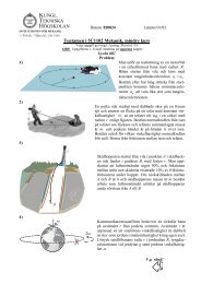
Figure 1.2: Schéma de la circulation océanique globale : aux pôles, le refroidissement<br />
en hiver et la formation de la glace de mer, qui tend à augmenter la salinité de l’eau<br />
libre, entraînent une augmentation de la densité et donc la mise en mouvement vertical<br />
des eaux superficielles qui plongent vers le fond. Tiré du site de l’INSU, CNRS.<br />
fréquence de Brunt-Väisälä varie de façon significative selon la verticale et cet effet<br />
peut avoir des conséquences importantes. Dans ce travail de thèse, on néglige cet<br />
aspect du problème et la pulsation N sera toujours considérée constante.<br />
A quel point les écoulements géophysiques sont-ils influencés par la stratification ?<br />
Pour répondre à cette question, quantifions les ordres de grandeur du nombre de<br />
Froude Fh = U/(NLh). On peut prendre pour vitesses et tailles caractéristiques respectivement<br />
U ∼ 10 m/s et Lh = 1000 km dans l’atmosphère et U ∼ 1 m/s et<br />
Lh = 100 km dans l’océan. Ces estimations mènent à des nombres de Froude de<br />
l’ordre de 10 −3 pour l’atmosphère et de 2 × 10 −3 pour l’océan. Ainsi, ces échelles sont<br />
fortement influencées par la stratification dans les deux milieux.<br />
Un autre effet structurant la dynamique des fluides géophysiques est la<br />
rotation de la terre avec une vitesse angulaire Ω0 ≃ 7.3 × 10 −5 rad/s. Du fait de<br />
la stratification et surtout du fait de la faible épaisseur de l’atmosphère et des océans<br />
par rapport au rayon terrestre et aux échelles horizontales, la rotation intervient au<br />
final à travers la composante horizontale de la force de Coriolis qui est proportionnelle<br />
à une pulsation f = 2Ω0 sin λ, fonction de la latitude λ. Selon le problème abordé,<br />
on peut considérer ou non la variation selon la latitude de f. Dans notre démarche<br />
d’idéalisation du problème, nous allons carrément négliger toute rotation d’ensemble.<br />
Pourquoi est-ce pertinent dans le contexte géophysique ? Il faut noter que le rapport<br />
N/f est généralement grand, de l’ordre de 10 ou 100. Cela signifie que la stratification<br />
influence une plus grande gamme d’échelles que la rotation et qu’il existe une gamme<br />
d’échelles influencée seulement par la stratification. Ainsi pour étudier la dynamique
6 CHAPITRE 1. INTRODUCTION GÉNÉRALE<br />
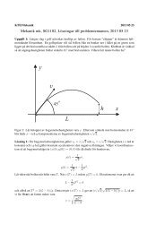
Figure 1.3: De la gauche vers la droite, spectres horizontaux de vents zonaux, de<br />
vents meridionaux et de température potentielle dans l’atmosphère (tropopause). Les<br />
spectres de vents méridionaux et de température ont été décalés de respectivement 1<br />
et 2 décades vers la doite. Tiré de Gage & Nastrom (1986).<br />
de ces échelles, on peut négliger la rotation d’ensemble. Notons enfin qu’à partir de la<br />
pulsation f, on construit un nombre sans dimension similaire au nombre de Froude, le<br />
nombre de Rossby Ro = U/(fLh) = (N/f)Fh quantifiant l’influence sur un écoulement<br />
de la rotation.<br />
Les ordres de grandeur du nombre de Reynolds dans les écoulements<br />
atmosphériques et océaniques sont très importants. Les viscosités cinématiques<br />
de l’air et de l’eau sont respectivement ν ≃ 10 −5 m 2 /s et ν ≃ 10 −6 m 2 /s.<br />
Ces valeurs associées aux valeurs de vitesse et taille caractéristiques mentionnées plus<br />
haut donnent des nombres de Reynolds de l’ordre de 10 12 pour l’atmosphère et 10 11<br />
pour les océans, c’est-à-dire tout à fait considérables. Cela signifie que les grandes<br />
échelles de ces écoulements sont très faiblement influencées par la dissipation et que<br />
les phénomènes non-linéaires de transferts entre échelles spatiales, comme par exemple<br />
le développement d’instabilité et la turbulence, sont fondamentaux. Précisons que les<br />
écoulements géophysiques sont très différents de la turbulence classique, observée par<br />
exemple dans le sillage d’une voiture. La turbulence dans les milieux géophysiques est<br />
très influencée par les effets structurants que sont la stratification et la rotation plané-
1.1. CONTEXTE ET MOTIVATIONS 7<br />
Figure 1.4: Spectres verticaux de cisaillement vertical dans l’océan. Les spectres sont<br />
normalisés par Φb = (ε KN) 1/2 et le nombre d’onde par kb = 1/lo, où ε K est le taux de<br />
dissipation d’énergie cinétique et lo est l’échelle d’Ozmidov (cf. section 1.4). Tiré de<br />
Gargett et al. (1981).<br />
taire. Les écoulements sont en terme de turbulence très intermittents spatialement et<br />
temporellement. Par exemple, des patches de turbulence à petites échelles sont observés<br />
dans les océans au sein d’un milieu globalement laminaire à petites échelles (Gregg,<br />
1987). En fait, le terme “turbulent” utilisé pour caractériser l’océan ou l’atmosphère,<br />
désigne des caractéristiques globales et statistiques concernant la répartition en énergie<br />
entre les différentes échelles de l’écoulement. Nous basons notre discussion sur des<br />
résultats concernant la répartition de l’énergie dans l’espace spectral. Puisque l’écoulement<br />
est anisotrope, plusieurs types de spectres doivent être utilisés. Par exemple,<br />
la figure 1.3 représente des spectres horizontaux (fonction d’un vecteur d’onde horizontal)<br />
de vitesse des vents et de température dans l’atmosphère tirés d’un article de<br />
Gage & Nastrom (1986). D’un autre côté, la figure 1.4 montre des spectres verticaux<br />
(fonction d’un vecteur d’onde vertical) de gradient vertical de vitesse obtenus par<br />
Gargett et al. (1981) par des lâchés d’appareils de mesures dans l’océan.<br />
Il nous faut mentionner un résultat fondamental pour ce qui nous concerne : il<br />
a été observé une importante régularité des spectres océaniques et atmosphériques<br />
(Riley & Lindborg, 2008). Des spectres de même type mesurés dans l’océan ou dans<br />
l’atmosphère, en différents endroits et moments sont généralement relativement similaires<br />
s’ils sont adimensionnés de manière adéquate. Par exemple, un spectre horizontal<br />
mesuré dans l’océan dans une certaine gamme d’échelles aura des caractéristiques générales<br />
communes avec les spectres de la figure 1.3. Ainsi en décrivant les figures 1.3<br />
et 1.4, on décrit aussi, indirectement, le spectre typique mesuré de manière récurrente<br />
dans l’atmosphère et les océans.<br />
Les spectres horizontaux présentés sur la figure 1.3 sont continus avec des pentes<br />
constantes correspondant à des lois d’échelle (caractéristiques typiques de la turbu-
8 CHAPITRE 1. INTRODUCTION GÉNÉRALE<br />
E(ki)<br />
10 10<br />
10 5<br />
10 0<br />
10 −5<br />
10 −10<br />
k −3<br />
h<br />
cascade<br />
d’enstropie,<br />
dynamique<br />
QG<br />
10 −4<br />
Ro ∼ 1<br />
k −5/3<br />
h<br />
cascade<br />
d’énergie,<br />
turbulence<br />
stratifiée<br />
10 −2<br />
k −3<br />
z<br />
F h ∼ 1<br />
khlo, kzlo<br />
10 0<br />
k −5/3<br />
cascade<br />
d’énergie,<br />
turbulence<br />
non-stratifiée<br />
Figure 1.5: Schéma simplifié des spectres anisotropes observés dans les fluides géophysiques<br />
de l’enveloppe terrestre. Les spectres horizontal (ligne bleu) et vertical (pointillés<br />
rouges) sont tracés en fonction des vecteurs d’onde normalisés par 1/lo. Les<br />
flèches symbolisent les différents types de cascade turbulente.<br />
lence). A très grande échelle (supérieures à ∼ 500 km), on a une loi de puissance en<br />
k −3<br />
h , c’est-à-dire un spectre très pentu avec beaucoup d’énergie aux grandes échelles<br />
par rapport au cas de la turbulence classique. Cette répartition énergétique selon les<br />
échelles horizontales s’explique par une dynamique de turbulence quasi-géostrophique,<br />
fortement influencée par la stratification et par la rotation terrestre (on reviendra en<br />
détail sur ce régime dans la section 1.4). Puis on observe une rupture de pente menant<br />
à un spectre en k −5/3<br />
h comme en turbulence classique. En fait, aux échelles relativement<br />
grandes supérieures à 100 m, cette pente ne peut pas s’interpréter en terme de turbulence<br />
classique : l’écoulement est bien trop influencé par la stratification. Notons que<br />
de tels spectres horizontaux sont maintenant reproduits numériquement grâce à des<br />
simulations numériques de l’atmosphère basées sur des codes plus ou moins idéalisés<br />
(Koshyk & Hamilton, 2001; Skamarock, 2004; Hamilton et al., 2008; Waite & Snyder,<br />
2009; Vallgren et al., 2012). Les spectres verticaux de gradient vertical de vitesse pré-<br />
sentés sur la figure 1.4 sont reliés au spectre vertical de vitesse par une division par<br />
kz 2 et la droite correspond à une loi d’échelle en k −3<br />
z . Nous voyons qu’aux grandes<br />
échelles verticales (associées à une pente en k −5/3<br />
en terme de spectre horizontal), les<br />
spectres verticaux sont en N 2 k −3<br />
z . Enfin, aux échelles relativement petites, on observe<br />
une rupture de pente menant à des spectres en k −5/3<br />
z<br />
h<br />
10 2<br />
gamme dissipative<br />
. Ainsi, contrairement au cas de<br />
la turbulence classique, les spectres atmosphériques et océaniques sont très fortement<br />
anisotropes : le spectre vertical est très différent du spectre horizontal. Le nombre<br />
de Froude horizontal associé à l’échelle où la rupture de pente a lieu (appelée échelle<br />
d’Ozmidov) est d’ordre 1. Cela explique pourquoi la turbulence redevient relativement<br />
isotrope et peu influencée par la stratification.
1.1. CONTEXTE ET MOTIVATIONS 9<br />
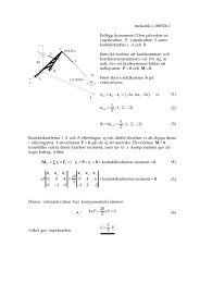
Figure 1.6: Champ de vorticité verticale obtenu par simulation numérique (Parallel<br />
Ocean Program) de l’Atlantique Nord. Tiré de Lapeyre (2010).<br />
Une représentation schématique des spectres anisotropes observés de façon relativement<br />
universelle dans la nature est présentée dans la figure 1.5. Les spectres horizontal<br />
et vertical sont superposés pour souligner l’anisotropie à grande échelle et le retour<br />
à l’isotropie aux plus petites échelles inférieures à l’échelle d’Ozmidov. Mentionnons<br />
enfin un résultat récent obtenu par Lindborg & Cho (2001) par des traitements fins<br />
de signaux mesurés lors de vols commerciaux d’avions de ligne (cf. chapitre 2). En<br />
reliant des quantités mesurées à la direction de la cascade, les auteurs ont montré que<br />
le régime inertiel lié aux spectres en k −5/3<br />
h était associé à une cascade d’énergie vers<br />
les petites échelles, comme en turbulence classique non influencée par la stratification.<br />
Structures cohérentes : ondes internes de gravité et tourbillons aplatis.<br />
Un fluide stratifié en densité est un milieu supportant la propagation d’ondes<br />
internes de gravité. Comme la houle propage de l’énergie à la surface des océans, ces<br />
ondes - qui peuvent être linéaires ou fortement non-linéaires - se propagent à l’intérieur<br />
de l’océan et de l’atmosphère. Ce mode de mouvement a été largement étudié<br />
et de nombreuses observations sont interprétées comme étant la signature d’ondes internes.<br />
En particulier, Garrett & Munk (1979) interprètent les spectres anisotropes<br />
océaniques par des superpositions d’ondes internes (sans expliquer dynamiquement la<br />
répartition en énergie entre ces ondes). D’un autre côté, il existe aussi des structures<br />
non-propagatives liées à des écoulements quasi-horizontaux et rotationels. Ces tourbillons<br />
intrinsèquement non-linéaires sont aussi largement observés dans la nature,<br />
notamment grâce à des bouées dérivantes (Gerin et al., 2009) et aux satellites (P. Y.<br />
Le Traon et al., 2008), et se retrouvent dans les simulations numériques d’écoulements<br />
géophysiques (cf. figure 1.6) 3 . Une caractéristique fondamentale de ces tourbillons<br />
est qu’ils sont fortement anisotropes et très aplatis. Historiquement, les deux types de<br />
mouvements ont souvent été considérés séparément, ou en interactions faibles. Dans ce<br />
travail de thèse, on s’intéresse en général à la dynamique turbulente des fluides strati-<br />
3 Notons que dynamique des méso-échelles dans la couche peu profonde des océans (environ les<br />
premiers 500m) s’interprète à l’aide du modèle quasi-géostrophique de surface (voir par exemple<br />
Lapeyre, 2010; Klein et al., 2008; P. Y. Le Traon et al., 2008)
10 CHAPITRE 1. INTRODUCTION GÉNÉRALE<br />
Figure 1.7: Photographie de l’atmosphère. La régularité observée sur les nuages est<br />
le signe du dévelopement d’une instabilité de cisaillement de type Kelvin-Helmholtz<br />
menant à un évènement de retournement.<br />
fiés à grand nombre de Reynolds sans considérer a priori de séparation stricte entre les<br />
modes propagatifs et non-propagatifs. En ce qui concerne la dynamique et la structure<br />
tridimensionnelle des moyennes et petites échelles, notons que des tourbillons d’axe<br />
horizontal liés à des instabilités de cisaillement (cf. figure 1.7) et des zones localisées<br />
de turbulence à très petites échelles sont couramment observés (Gregg, 1987).<br />
Nous avons déjà souligné que la modélisation numérique des systèmes océaniques<br />
et atmosphériques (modèles de circulation générale, GCM et modèles régionaux) était<br />
un outil très important pour la compréhension et la prédiction dans les sciences des<br />
enveloppes fluides des planètes. La nature même des systèmes à simuler qui sont très<br />
complexes et à très grands nombres de degrés de liberté implique qu’il est absolument<br />
impossible de tout calculer de façon exacte. Chaque simulation numérique est donc<br />
basée sur des simplifications et des modélisations des échelles et phénomènes nonrésolus.<br />
C’est le principe des LES (“Large Eddy Simulation”, ou simulation des grands<br />
tourbillons) mais avec des écoulements turbulents fortement influencés par des effets<br />
structurants, dont en premier lieu la stratification en densité. Pour modéliser au mieux<br />
les phénomènes “sous-mailles” (non-résolus), il faut insérer à la main leur dynamique<br />
physique. Cette étape de modélisation est critique car les simulations sont fortement<br />
sensibles aux modèles sous-mailles (Bryan, 1987; Goosse et al., 1999). Dans le cadre<br />
de cette problématique, il est donc fondamental d’avoir une bonne compréhension de<br />
la dynamique de la turbulence fortement influencée par une stratification en densité.<br />
Dans les prochaines sections, on introduit les éléments nécessaires à la bonne compréhension<br />
de ce travail de thèse. On propose une présentation globale des problématiques<br />
liées à la dynamique des fluides stratifiés et tournants à grand nombre de<br />
Reynolds. Pour être accessible aux non-spécialistes, cette présentation est conduite à<br />
partir de concepts de base de l’hydrodynamique. Notre modèle de travail est présenté<br />
dans la prochaine section. On abordera ensuite le sujet de la turbulence classique tridimensionnelle<br />
puis bidimensionnelle (section 1.3). Enfin, on proposera un tour d’horizon<br />
de la riche dynamique des fluides stratifiés en densité et tournants (section 1.4).
1.2. MODÈLE : FLUIDE INCOMPRESSIBLE NEWTONIEN STRATIFIÉ 11<br />
1.2 Modèle : fluide incompressible newtonien stratifié en<br />
densité<br />
Pour rentrer dans le vif du sujet de la dynamique des écoulements turbulents dans<br />
les fluides stratifiés, nous allons nous appuyer sur les équations fondamentales qui la<br />
décrivent. A un certain degré d’approximation, ces équations s’expriment simplement.<br />
En revanche, leur résolution pose des problèmes fondamentaux. Nous verrons qu’il<br />
faudra soit procéder à des approximations et à des développements en terme de petits<br />
paramètres, soit utiliser l’outil numérique pour les simuler. Mais d’abord, présentons<br />
notre modèle de travail, les approximations sous-jacentes et les équations associées.<br />
1.2.1 Approximation de Boussinesq<br />
La dynamique d’un fluide newtonien stratifié en densité est, lorsque la vitesse est<br />
relativement faible devant la vitesse du son et que les variations de densité sont relativement<br />
faibles devant la densité moyenne, régie par les équations de Navier-Stokes<br />
dans l’approximation de Boussinesq 4 . Partons des équations classiques des milieux<br />
continus : (i) l’équation exprimant la conservation de la masse<br />
dρtot<br />
dt + ρtot∇ · u = 0, (1.1)<br />
où ρtot est la masse volumique totale du fluide, u la vitesse et d/dt = ∂t + u · ∇ la<br />
dérivée particulaire ; (ii) l’équation exprimant la conservation de l’impulsion pour un<br />
fluide newtonien, i.e. l’équation de Navier-Stokes<br />
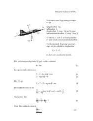
du<br />
ρtot<br />
dt = −∇˜p − ρtotgez + ρtotf + ρtotν∇ 2 u, (1.2)<br />
où ˜p est la pression, ez le vecteur unitaire vertical orienté vers le haut, f inclu toutes<br />
les forces massiques et ν est la viscosité cinétique (une diffusivité). Nous avons comme<br />
variables un champ vectoriel (la vitesse) et deux champs scalaires (la pression et la<br />
densité totale). Pour fermer le système il manque donc une équation scalaire. Nous<br />
l’introduirons plus tard à partir de la thermodynamique.<br />
L’approximation de Boussinesq est basée sur une décomposition de la densité totale<br />
ρtot en une densité moyenne ρ0, un profil ρ(z) intégrant la stratification de base, et<br />
une fonction ρ ′ (x) correspondant aux perturbations de densité : ρtot = ρ0 + ρ(z) + ρ ′ .<br />
Cette approximation consiste à remplacer partout, sauf dans le terme de flottabilité,<br />
la densité totale par la densité de référence ρ0. Cela peut paraître assez brutal mais<br />
cela se justifie si certaines conditions sont remplies (voir par exemple Cushman-Roisin,<br />
1994; Staquet, 1998). En plus de la condition liée à l’incompressibilité (vitesses très<br />
inférieures à la célérité du son), une condition supplémentaire de faible variation de<br />
4 Dans ce travail de thèse, on utilisera toujours cette approximation. Notons qu’elle n’est pas<br />
adaptée à la description de la dynamique de l’atmosphère. L’approximation anélastique, qui intègre<br />
des effets de compressibilité mais pas les ondes acoustiques, est couramment utilisée et mène à des<br />
équations très similaires.
12 CHAPITRE 1. INTRODUCTION GÉNÉRALE<br />
la densité, ρ(z) et ρ ′ ≪ ρ0, doit être remplie. L’approximation de Boussinesq est<br />
très couramment utilisée notamment pour l’étude des océans où ces conditions sont<br />
largement remplies.<br />
Le système d’équation se réduit à l’équation de Navier-Stokes incompressible avec<br />
un terme de flottabilité<br />
du<br />
dt<br />
= −∇ ˜p<br />
ρ0<br />
− ρtotg<br />
ez + f + ν∇<br />
ρ0<br />
2 u, (1.3)<br />
et à la condition de divergence nulle ∇ · u = 0. En soustrayant à l’équation (1.3) sa<br />
solution d’équilibre au repos 0 = −∂z ˜pstat/ρ0 − g(ρ0 + ρ(z))/ρ0, on obtient<br />
du<br />
dt = −∇p − ρ′ g<br />
ez + f + ν∇<br />
ρ0<br />
2 u, (1.4)<br />
où p ≡ (˜p − ˜pstat)/ρ0 est une pression redimensionnée en énergie par unité de masse.<br />
Pour fermer le système, on doit considérer les causes de la variation de masse<br />
volumique. Classiquement, les variations de densité sont liées à des variations de température<br />
T , de salinité S et dans le cas d’un gaz, de pression. Dans une certaine<br />
gamme de variations relativement faibles, une équation d’état linéaire de la forme<br />
ρtot = ρ0[1 − α(T − T0) + β(S − S0)] s’applique avec α le coefficient d’expansion<br />
thermique et β le coefficient de contraction haline. A ce niveau d’approximation, les<br />
dynamiques des variables thermodynamiques T et S sont décrites par une équation<br />
d’advection-diffusion (découlant de la conservation de l’énergie pour la température<br />
et de la quantité de matière pour la salinité, voir par exemple Rieutord, 1997). Si l’on<br />
considère le cas où la stratification est liée à la variation d’une seule variable thermodynamique<br />
(par exemple la salinité), on a une simple relation de proportionnalité de<br />
type ρtot = ρ0[1+β(S −S0)] et l’équation d’advection-diffusion s’applique à la densité<br />
totale<br />
dρtot<br />
dt = κ∇2 ρtot, (1.5)<br />
où κ est la diffusivité. Dans l’équation (1.4), la quantité flottabilité b = −ρ ′ g/ρ0<br />
apparaît. On obtient son équation d’évolution en utilisant la décomposition de la<br />
densité totale introduite plus haut et l’équation (1.5)<br />
d ρ<br />
dt<br />
′ g<br />
+ w<br />
ρ0<br />
g dρ<br />
ρ0 dz = κ∇2 ρ ′ g<br />
. (1.6)<br />
ρ0<br />
On voit que la quantité gdzρ/ρ0, proportionnelle au gradient moyen de densité, caractérise<br />
le couplage entre le champ de vitesse et les variables thermodynamiques.<br />
Ainsi on définit la pulsation caractéristique du milieu stratifié en densité appelée fréquence<br />
de Brunt-Väisälä N = −gdzρ/ρ0. Notons que la mal-nommée “fréquence” 5<br />
de Brunt-Väisälä est bien une pulsation avec une période associée égale à 2π/N.<br />
Selon le contexte, plusieurs variables thermodynamiques sont utilisées. La fonction<br />
perturbations de densité ρ ′ est adaptée au contexte de l’expérimentation. Dans l’atmosphère,<br />
la fonction fluctuations de température potentielle θ, i.e. la température<br />
5 En anglais, le mot frequency désigne indifféremment une fréquence ou une pulsation.
1.2. MODÈLE : FLUIDE INCOMPRESSIBLE NEWTONIEN STRATIFIÉ 13<br />
compensée de l’effet des transformations adiabatiques, est utilisée (voir par exemple<br />
Pedlosky, 1987). La flottabilité b = −gρ ′ /ρ0 (ou son opposé appelée “densité réduite”<br />
et notée σ) qui a un sens physique d’accélération, est couramment considérée. Dans<br />
ce manuscrit, on préférera souvent utiliser ζ ≡ ρ ′ /|dzρ| = gρ ′ /(N 2 ρ0), le déplacement<br />
vertical des particules fluides par rapport à l’état au repos. Le sens physique de<br />
longueur verticale permet des comparaisons simples avec toutes les autres longueurs<br />
caractéristiques importantes dans le problème. Cette variable ζ est aussi employée dans<br />
le code numérique que nous avons utilisé (ns3d, cf. chapitre A). La décomposition de<br />
la densité totale en fonction du déplacement vertical ζ s’écrit<br />
ρtot = ρ0 + ρ(z) + |dzρ|ζ. (1.7)<br />
Finalement, en utilisant pour variable thermodynamique le déplacement vertical<br />
ζ, on obtient :<br />
∂u<br />
∂t + u · ∇u = −∇p − N 2 ζez + ν∇ 2 u, (1.8)<br />
∂ζ<br />
∂t + u · ∇ζ = +w + κ∇2 ζ. (1.9)<br />
Le terme de flottabilité brise l’isotropie des équations. La direction verticale devient<br />
une direction privilégiée et on peut anticiper le fait que les structures hydrodynamiques<br />
sont anisotropes. Par contre nous pourrons nous appuyer sur l’axisymétrie des<br />
équations, i.e. leur invariance par rotation autour de l’axe vertical.<br />
Tous les résultats présentés dans ce manuscrit concernent le cas d’un fluide stratifié<br />
sans rotation. Cependant, on va considérer dans ce chapitre introductif l’effet<br />
de la rotation en introduisant une rotation d’ensemble du référentiel de travail, de<br />
vecteur rotation Ω = Ωez avec Ω constant (c’est l’approximation dite “plan f”). La<br />
rotation fait apparaître des termes supplémentaires dont une partie peut s’intégrer<br />
dans le terme de pression. Seule reste la force de Coriolis dont l’expression (en terme<br />
d’accélération massique) est −2Ω×u = −fez ×u, où f = 2Ω est la pulsation associée<br />
à la rotation.<br />
1.2.2 Formulation dans l’espace spectral<br />
Nous allons couramment utiliser la version du système d’équations (1.8-1.9) dans l’espace<br />
spectral. Nous présentons notamment de nombreux résultats tirés de simulations<br />
numériques directes effectuées grâce à un code numérique pseudo-spectral basé sur la<br />
transformée de Fourier (cf. chapitre A). L’espace de Fourier présente quatre avantages<br />
importants : (i) les opérateurs différentiels linéaires s’y expriment très simplement, (ii)<br />
la condition de divergence nulle s’interprète de façon géométrique, (iii) elle permet une<br />
très bonne précision numérique et (iv) il existe un algorithme très efficace de transformée<br />
de Fourier appelé “Fast Fourier Transform”, ou FFT, de complexité n ln n, où<br />
n est le nombre de points de colocation. Le désavantage majeur de la transformation<br />
de Fourier est qu’elle est basée sur une symétrie de translation dans l’espace physique<br />
(espace infini ou périodique) incompatible avec des parois de forme non-triviale.
14 CHAPITRE 1. INTRODUCTION GÉNÉRALE<br />
Ainsi, dans la suite, on considérera un espace sans paroi et périodique dans les trois<br />
dimensions.<br />
Transformée de Fourier 1D : quelques définitions On doit adopter une convention<br />
pour la transformée de Fourier. On choisit la définition correspondant à un espace<br />
physique continu et périodique et donc un espace spectral discret et infini. Soit f une<br />
fonction réelle d’un espace physique unidimensionel et périodique sur l’intervalle [0 Lx],<br />
ˆf(kl) = T F1D[f](kl) la série de Fourier associée, avec kl = k1l, l ∈ Z et k1 = 2π/Lx.<br />
Alors la fonction dans l’espace physique et la série de Fourier sont reliées par les<br />
relations<br />
Lx<br />
ˆf(kl) = f(x)e<br />
0<br />
−iklx<br />
dx/Lx, (1.10)<br />
f(x) = <br />
ˆf(kl)e iklx<br />
. (1.11)<br />
l<br />
En pratique, numériquement et physiquement avec l’échelle de coupure visqueuse,<br />
la résolution spatiale est limitée et l’espace des nombres d’onde est borné. Si l’on a Nx<br />
points de co-location dans l’espace physique pour la direction x, l’indice l est limité à<br />
l’intervalle [−Nx/2 + 1 Nx/2] et le nombre d’onde maximal est kmax = k1Nx/2.<br />
L’énergie moyenne associée au champ réel f(x),<br />
Ef = 〈f 2 /2〉 = 1<br />
Lx<br />
f(x)<br />
2 0<br />
2 dx/Lx, (1.12)<br />
où les crochets 〈·〉 signifient une moyenne, s’exprime dans l’espace spectral en vertu du<br />
théorème de Parseval comme une somme : Ef = <br />
l | ˆ f(kl)| 2 /2. On définit le spectre<br />
associé au champ f, E(kl) comme la densité spectrale d’énergie6 , c’est-à-dire que<br />
Ef = <br />
E(kl)k1. (1.13)<br />
kl0<br />
Cette somme tend dans la limite k1 → 0 vers l’intégrale <br />
E(k)dk, ce qui signifie<br />
k>0<br />
que le spectre discret E(kl) converge vers le spectre continu E(k). Par identification,<br />
on trouve que E(kl) = | ˆ f(kl)| 2 /k1.<br />
Rappelons enfin qu’une analyse en échelle peut être faite de manière équivalente<br />
dans le domaine physique avec la fonction de corrélation Cf (r) = 〈f(x)f(x + r)〉. On<br />
montre que le spectre de la fonction de correlation<br />
<br />
dr dx<br />
Ĉf (k) =<br />
f(x)f(x + r)e −ikr , (1.14)<br />
Lx<br />
Lx<br />
est intimement lié à la corrélation et que l’on a Ĉf(k) = | ˆ f(k)| 2 . Concrètement<br />
l’analyse est souvent faite en terme de fonctions de structure d’ordre deux S2(r) =<br />
〈[δf(r)] 2 〉 = 2〈f 2 〉−2Cf(r), où δf(r) = f(x+r)−f(x) est l’incrément de la fonction f.<br />
6 Dans le chapitre A, on définit précisement les différents spectres utilisés (1D, 2D, etc.).
1.2. MODÈLE : FLUIDE INCOMPRESSIBLE NEWTONIEN STRATIFIÉ 15<br />
Transformée de Fourier et opérateurs non-linéaires Bien sûr, les écoulements<br />
stratifiés évoluent dans un espace à trois dimensions. On utilisera donc majoritairement<br />
la transformée de Fourier 3D et le chapeau (ˆ) signifiera la plupart du temps cette<br />
transformation. Ainsi, û = T F3D[u] est la série de Fourier 3D de la vitesse u. On va<br />
appliquer maintenant cette transformation au système d’équations (1.8-1.9).<br />
Les opérateurs linéaires s’expriment très simplement dans l’espace de Fourier avec<br />
en particulier ∂mf = ikm ˆ f. Ainsi la condition d’incompressibilité s’exprime simplement<br />
de façon géométrique k · û = 0. Le champ de vitesse est dit solénoïdal, ce qui<br />
signifie que dans l’espace de Fourier, il est orthogonal au vecteur d’onde et peut être<br />
décrit par seulement deux composantes.<br />
Par contre il n’en va pas de même des termes non-linéaires car l’on a fg = ˆ f ∗ ˆg, où<br />
∗ symbolise la convolution, opérateur intégral pour lequel il n’existe pas d’algorithme<br />
rapide similaire à la FFT. Numériquement, il est plus avantageux de calculer les termes<br />
non-linéaires en revenant dans l’espace physique, c’est-à-dire en utilisant la formule<br />
T F [fg] = T F<br />
<br />
T F −1 [ ˆ f]T F −1 <br />
[ˆg] . (1.15)<br />
Les codes numériques utilisant cette stratégie de calcul sont dits pseudo-spectraux.<br />
L’algorithme FFT est central dans ce type de code et il devra être correctement<br />
optimisé pour obtenir de bonnes performances. Pour plus de concision, on définit<br />
deux quantités non-linéaires nl ≡ u · ∇u et nlP ≡ u · ∇ζ. L’équation d’évolution des<br />
modes de Fourier de la vitesse s’écrit<br />
∂tû + nl = −ikˆp − N 2ˆ ζez − νk 2 û. (1.16)<br />
Notons que certains termes de cette équation ne sont pas perpendiculaires au vecteur<br />
d’onde. Pour respecter la condition d’incompressibilité k · û = 0, la pression s’adapte<br />
instantanément et de façon non-locale 7 et l’on a<br />
i|k| 2 ˆp = −k · ( nl + N 2ˆ ζez). (1.17)<br />
Ainsi, si l’on ne s’intéresse pas en soit à la pression, on peut oublier ces termes et ne<br />
considérer que les composantes perpendiculaires au vecteur d’onde. On utilise pour<br />
cela le tenseur P⊥ = δ − ek ⊗ ek·, où δ est la matrice identité et ek le vecteur<br />
unitaire colinéaire à k, de projection sur le plan perpendiculaire au vecteur d’onde.<br />
Avec ces notations, le système d’équations (1.8-1.9) devient dans l’espace de Fourier<br />
∂tû = P⊥[− nl − N 2ˆ ζez] −ν|k| 2 û, (1.18)<br />
∂t ˆ ζ = − nlP + ˆw −κ|k| 2ˆ ζ. (1.19)<br />
Remarquons que cette formulation ne fait pas intervenir la pression, que l’on ne calcule<br />
donc pas explicitement.<br />
7 Ce résultat étrange est lié à l’approximation d’incompressibilité. En réalité, les ondes de pression<br />
se propagent à une vitesse finie, la vitesse du son.
16 CHAPITRE 1. INTRODUCTION GÉNÉRALE<br />
1.3 Turbulence dans les fluides non-stratifiés, 3D et 2D<br />
Dans cette section on présente quelques résultats majeurs concernant la turbulence<br />
classique, c’est-à-dire non influencée par un effet structurant comme la stratification.<br />
La turbulence est un problème fondamental de l’hydrodynamique et plus généralement<br />
de l’étude des systèmes non-linéaires et multi-échelles. C’est un domaine très étudié<br />
pour son intérêt pratique (une très grande part des écoulements aux échelles humaines<br />
et supérieures ont de fortes tendances à la turbulence) mais aussi pour son intérêt<br />
théorique. On va ici brosser un tableau très rapide, en se focalisant sur ce qui va<br />
nous intéresser pour la suite du manuscrit. On se cantonne au cas incompressible<br />
décrit par l’équation de Navier-Stokes incompressible (équation (1.8) sans le terme de<br />
flottabilité). On s’intéresse d’abord au cas classique tridimensionnel.<br />
1.3.1 Turbulence 3D<br />
Cascade de Richardson et invariance du flux d’énergie entre échelles<br />
Au début du chapitre 1, on a déjà introduit le concept de cascade de Richardson.<br />
Précisons cette notion dans le cas de la turbulence statistiquement stationnaire tridimensionnelle.<br />
Un mécanisme d’injection d’énergie force des structures hydrodynamiques<br />
de grande échelle, i.e. associées à un grand nombre de Reynolds et donc<br />
faiblement influencées par la dissipation. Le taux d’injection d’énergie est d’ordre<br />
P ∼ U 2 /T ∼ U 3 /L (unité d’énergie massique par unité de temps), où U, T et L<br />
sont respectivement la vitesse, le temps et la taille caractéristiques des plus grandes<br />
structures de l’écoulement (échelle dite intégrale). L’énergie ne peut pas être dissipée à<br />
l’échelle de forçage et les grandes structures hydrodynamiques évoluent sur un temps<br />
long, de l’ordre de quelques temps caractéristiques T . Ainsi, les mécanismes inertiels<br />
non-linéaires, c’est-à-dire d’interactions entre échelles, ont le temps de transférer efficacement<br />
l’énergie vers des petites échelles. Ce processus se répète sur toute une<br />
gamme d’échelles de manière relativement invariante avec un certain flux d’énergie<br />
entre échelles Π(l) ∼ u(l) 3 /l, où l correspond à une échelle de la cascade et u(l) la<br />
vitesse caractéristique associée. Considérons deux échelles proches dans la cascade l1<br />
et l2 < l1 telles que l’échelle l1 transfert son énergie vers l’échelle l2. Si Π(l2) < Π(l1),<br />
l’énergie s’accumule à l’échelle l2 et Π(l2) ∼ u(l2) 3 /l2 augmente (la turbulence n’est<br />
pas statistiquement stationnaire). Un équilibre dynamique statistiquement stationnaire<br />
est atteint lorsque le flux est égal pour chaque échelle. On a alors Π = P sur<br />
toute la cascade et u(l) = (Πl) 1/3 (Taylor, 1935).<br />
Au fur et à mesure de la cascade, l’énergie est contenue dans des structures hydrodynamiques<br />
liées à des nombres de Reynolds Re(l) ∼ u(l)l/ν ∼ Π 1/3 l 4/3 /ν de plus en<br />
plus petits. A une certaine échelle appelée échelle de Kolmogorov, les gradients sont<br />
si importants que l’énergie est dissipée en chaleur avec un certain taux de dissipation<br />
d’énergie massique ε. Si l’on postule l’invariance d’échelle et la stationnarité statistique,<br />
on obtient une version qualitative d’un résultat tout à fait fondamental, l’égalité<br />
entre le taux d’injection, de transfert et de dissipation d’énergie :<br />
P = U 3 /L = Π = u(l) 3 /l = ε. (1.20)
1.3. TURBULENCE DANS LES FLUIDES NON-STRATIFIÉS, 3D ET 2D 17<br />
Ce résultat, valable pour un nombre de Reynolds suffisamment important, implique<br />
que la dissipation est invariante par modification de la viscosité du fluide. C’est seulement<br />
la taille des structures dissipatives, c’est-à-dire l’échelle de Kolmogorov, qui<br />
est modifiée. On peut évaluer cette échelle η, pour laquelle Re(η) ∼ 1 et on trouve<br />
η = (ν 3 /ε) 1/4 ∼ LRe −3/4 .<br />
Limitation à une description statistique, probabiliste<br />
Nous avons vu qu’un système d’équations de formulation relativement simple décrit<br />
parfaitement la dynamique de la turbulence incompressible. Pourtant on vient de<br />
voir qu’un des résultats clés est d’ordre statistique. Nous sommes limités à une telle<br />
description par des difficultés d’ordre fondamental et pratique. Elles sont liées en particulier<br />
à deux ingrédients présents : les non-linéarités et la non-localité induite par le<br />
terme de pression. D’abord, il n’existe pas de solution analytique correspondant à un<br />
champ de vitesse turbulent. De toute façon, la non-linéarité implique des comportements<br />
chaotiques, avec sensibilité aux conditions initiales et divergence des trajectoires<br />
dans l’espace des phases. La turbulence est aussi caractérisée par une superposition<br />
de structures hydrodynamiques d’échelles très différentes. On est donc dans le cas de<br />
chaos à très grand nombre de degrés de liberté 8 .<br />
Ainsi la description de l’état d’un écoulement turbulent demande une très grande<br />
quantité d’informations ce qui mène à des difficultés concrètes considérables. En première<br />
approximation, ce nombre de degrés de liberté peut être quantifié par le nombre<br />
de points numériques nécessaires à la simulation d’un écoulements turbulent. Avec un<br />
point par volume de Kolmogorov η 3 , il faut pour résoudre un volume caractéristique<br />
d’échelle intégrale L 3 , de l’ordre de (η/L) 3 ∼ Re 9/4 points de colocation. Cette loi<br />
d’échelle mène très vite pour des écoulements réels à grand nombre de Reynolds à des<br />
quantités de points de calcul nécessaires totalement hors de portée même des ordinateurs<br />
les plus puissants. Néanmoins les progrès techniques sont remarquables et des<br />
simulations à très hautes résolutions ont été réalisées. En 2011, les plus grosses simulations<br />
ont des résolutions de l’ordre de 4096 3 . Ces calculs représentent de véritables<br />
exploits techniques et ouvrent des horizons nouveaux en terme d’analyse et de compréhension<br />
de la dynamique des écoulements turbulents. La taille mémoire d’un champ de<br />
vitesse donne une petite idée de la difficulté de ce type de calculs (et des traitements<br />
des données). Avec la précision nécessaire (8 octets par valeur numérique), un champ<br />
vectoriel en trois dimensions représente approximativement 8 × 3 × 4096 3 ∼ 1650 Go<br />
à manipuler 9 .<br />
Pour toutes ces raisons théoriques et pratiques, et alors qu’aucun effet non classique<br />
(relativiste et/ou quantique) n’entre en jeu, nous sommes fondamentalement réduits<br />
à une description statistique et probabiliste de la turbulence. Ainsi, l’étude de la<br />
turbulence est intimement liée à la science du traitement statistique des signaux.<br />
Certains outils complexes sont utilisés (par exemple les ondelettes ou les fractales) mais<br />
8 En opposition au chaos à petits nombres de degrés de liberté qui caractérise certains systèmes<br />
très simples mais fortement non-linéaires, par exemple le pendule double.<br />
9 A comparer à la taille mémoire des plus gros disques durs disponibles au grand public, de l’ordre<br />
de 1000 Go.
18 CHAPITRE 1. INTRODUCTION GÉNÉRALE<br />
dans ce travail de thèse, on se limite à quelques concepts classiques. Après la moyenne<br />
et l’écart type, une des quantités statistiques la plus simple et facilement accessible<br />
dans l’expérience est la fonction de structure d’ordre 2 des incréments de vitesse<br />
S2(r) = 〈[δu] 2 〉 (reliée simplement aux corrélations de vitesse). On a vu que sous<br />
des hypothèses d’invariance par translation (ou de périodicité), la transformation de<br />
Fourier était très utile. Il existe alors un parallélisme parfait entre les deux descriptions<br />
spatiale et spectrale qui sont liées par la relation Ĉu(k) = |û| 2 (k) (cf. paragraphe<br />
d’introduction de la transformée de Fourier plus haut).<br />
Dans ce cadre statistique, les difficultés inhérentes aux non-linéarités apparaissent<br />
avec le problème fondamental de fermeture des équations statistiques. Les équations<br />
d’évolution des quantités d’ordre 2 (fonctions de structure d’ordre 2, corrélations et<br />
spectres, liés à la répartition de l’énergie entre les échelles spatiales) sont fonctions<br />
de quantités d’ordre 3, et ainsi de suite sans fin. Pour fermer les équations il n’y a<br />
pas d’autres solutions que de faire des approximations consistant à exprimer de façon<br />
ad-hoc une quantité d’un certain degré en fonction d’une quantité d’ordre inférieur<br />
(par exemple avec une approche de type EDQNM 10 ).<br />
Comme souvent en physique, les piliers pour l’analyse proviennent des symétries :<br />
d’abord avec les quantités conservées, liées à des invariances des équations, par exemple<br />
l’énergie associée à l’invariance par translation temporelle des équations ; ensuite avec<br />
les symétries du milieu et des conditions limites. En particulier, la turbulence statistiquement<br />
homogène et isotrope a une importance fondamentale qui va bien au delà des<br />
cas où le forçage est lui même homogène et isotrope. En effet, les processus de cascade<br />
entre échelles ont tendance à faire perdre la mémoire de la forme précise du forçage.<br />
Lorsque le nombre de Reynolds est suffisamment grand et la cascade est suffisamment<br />
profonde (L/η ≫ 1), la turbulence devient localement statistiquement homogène et<br />
isotrope, et finalement “universelle” : la structure et la dynamique de la turbulence<br />
ne dépendent plus de la forme du forçage à grande échelle (pour une discussion sur ce<br />
point, voir par exemple Mininni et al., 2006).<br />
Lois de Kolmogorov pour la turbulence homogène isotrope<br />
Kolmogorov (1941b) a dérivé un ensemble de résultats fondateurs, dont en particulier<br />
une loi exacte dans la limite d’un très grand nombre de Reynolds. Comme la relation<br />
dimensionnelle (1.20), cette loi exacte, dite “loi des 4/5”, exprime l’égalité entre flux<br />
d’énergie dans la cascade et dissipation. Elle a pour expression classique<br />
〈[δvL(r)] 3 〉 = − 4<br />
εr, (1.21)<br />
5<br />
où δvL(r) = (u(x+r)−u(x))·r/r est l’incrément de vitesse longitudinale. Cette loi relie<br />
une quantité d’ordre 3 associée aux transferts d’énergie entre échelles à la dissipation.<br />
On discute de ce sujet de façon plus approfondie dans l’introduction du chapitre 5.<br />
Le flux d’énergie à travers les échelles (dans le domaine spectral) obtenu pour une<br />
simulation numérique d’écoulement turbulent forcé est représenté sur la figure 1.8. On<br />
10 Eddy-Damped Quasi-Normal Markovian, voir Sagaut & Cambon (2008).
1.3. TURBULENCE DANS LES FLUIDES NON-STRATIFIÉS, 3D ET 2D 19<br />
Figure 1.8: Flux d’énergie entre les échelles en fonction du module du vecteur d’onde.<br />
Tiré de Mininni et al. (2006).<br />
voit que cette quantité est pratiquement constante dans le domaine inertiel (domaine<br />
dans lequel l’inertie domine et la dissipation est très faible), ce qu’exprime la loi des<br />
4/5 dans l’espace physique.<br />
De la loi exacte des 4/5 (ou de la relation dimensionnelle 1.20), on tire sous l’hypothèse<br />
de normalité (distribution de probabilité gaussienne) des prédictions pour la<br />
forme des fonctions de structure d’ordre 2 et des spectres<br />
〈[δvL(r)] 2 〉 = C ′ ε 2/3 r 2/3 , E(k) = Cε 2/3 k −5/3 , (1.22)<br />
où C ′ et C sont des constantes universelles dites de Kolmogorov. Ces relations, qualifiées<br />
de lois des 2/3 et des 5/3 respectivement, sont vérifiées expérimentalement et<br />
numériquement avec un bon accord. Notamment, une variation du spectre en k −5/3<br />
est une caractéristique particulièrement robuste de nombreux écoulements turbulents<br />
(voir la figure 1.9). Dans l’annexe A, on précisera les définitions de différents types de<br />
spectres. On pourra alors donner des valeurs numériques des constantes de Kolmogorov<br />
associées.<br />
Remarquons qu’en s’intéressant aux variations des moments supérieurs de la distribution<br />
des incréments de vitesse, on a montré que l’hypothèse de normalité n’était<br />
pas valide (Oboukhov, 1962; Kolmogorov, 1962). La turbulence est très intermittente<br />
avec des probabilités d’événements forts déviant significativement de la loi gaussienne<br />
(voir par exemple Chevillard et al., 2006).<br />
Structures cohérentes, mécanismes de la cascade turbulente et vorticité<br />
Même si la caractérisation globale de la turbulence est statistique, on peut apprendre<br />
beaucoup en étudiant la dynamique dans l’espace physique des structures cohérentes<br />
(tourbillons, nappes de cisaillement, etc.). Dans cette introduction, on ne discute<br />
pas des mécanismes possiblement à l’origine de la cascade turbulente en milieu nonstratifié.<br />
On pourrait notamment se baser sur une analyse des instabilités agissant<br />
sur des structures de base de l’écoulement, par exemple l’instabilité elliptique sur un<br />
tourbillon ou l’instabilité de cisaillement (dite de Kelvin-Helmholtz) sur une nappe de
20 CHAPITRE 1. INTRODUCTION GÉNÉRALE<br />
Figure 1.9: Spectres de vitesse d’écoulement turbulent. Tiré de Saddoughi & Veeravalli<br />
(1994) où les références des différentes expériences sont données.<br />
cisaillement. Ces instabilités mènent à des transferts d’énergie vers des petites échelles<br />
et finalement à la transition à la turbulence. La figure 1.10 illustre le cas de l’instabilité<br />
cisaillement (dite de Kelvin-Helmholtz dans le cas stratifié).<br />
Ici, on va se limiter à montrer comment la grandeur vorticité ω = ∇ × u qui<br />
caractérise la rotation locale d’une particule fluide permet d’interpréter des processus<br />
hydrodynamiques à la base de la cascade turbulente. L’équation d’évolution de la<br />
vorticité<br />
dω<br />
dt = ω · ∇u + ν∇2 u, (1.23)<br />
comporte trois termes : elle est advectée par le champ de vitesse (terme de gauche),<br />
étirée et inclinée par les gradients de vitesse (terme ω · ∇u) et enfin dissipée par la<br />
viscosité. Aux effets visqueux près, sa dynamique est identique à celle d’un vecteur<br />
reliant deux points matériels advectés par l’écoulement. Nous allons montrer que le<br />
terme d’étirement de la vorticité est fondamental pour la cascade d’énergie vers les<br />
petites échelles.<br />
Dans un premier temps, notons qu’une cascade turbulente est liée à une forte<br />
concentration de la vorticité aux petites échelles de l’écoulement. On peut quantifier<br />
cette concentration en considérant la dissipation moyenne. Localement la dissipation
1.3. TURBULENCE DANS LES FLUIDES NON-STRATIFIÉS, 3D ET 2D 21<br />
Figure 1.10: Destabilisation d’une couche de cisaillement par l’instabilité de Kelvin-<br />
Helmholtz. Des tourbillons d’axe horizontal sont formés lors de l’évolution non-linéaire<br />
de l’instabilité menant finalement à la transition à la turbulence. Le schéma (a) est<br />
tiré de Morize (2006) et l’expérience de Falkovich & Sreenivasan (2006).<br />
ε(x) = 2νSijSij est liée aux déformations, donc aux gradients symétriques de vitesse<br />
Sij = (∂iuj +∂jui)/2. Mais dans un fluide incompressible, on peut relier la dissipation<br />
moyenne au champ de vorticité ε = 〈ε(x)〉 = 2νZ, où Z = 〈|ω| 2 /2〉 est l’enstrophie,<br />
la quantité quadratique associée à la vorticité. On en déduit que pour respecter l’invariance<br />
de la dissipation par variation de la viscosité, on doit avoir Z ∼ (U/L) 2 Re.<br />
Ainsi, plus le nombre de Reynolds est grand, plus la vorticité se concentre aux petites<br />
échelles.<br />
On peut par exemple considérer un processus de transition à la turbulence à partir<br />
d’une grande structure hydrodynamique laminaire. Une telle transition à la turbulence<br />
implique une série d’instabilités menant in fine au développement de structures<br />
dissipatives de très petites tailles (voir figure 1.10). Ce processus est associé à une<br />
augmentation de l’enstrophie saturant finalement à une valeur de l’ordre de (U/L) 2 Re<br />
puisqu’alors l’écoulement est fortement dissipatif et la turbulence décline rapidement.<br />
A partir de l’équation (1.23), on montre que<br />
dZ<br />
dt = 〈ω · (ω · ∇)u〉 − ν〈∂iωj∂iωj〉 (1.24)<br />
ce qui prouve qu’une telle augmentation de l’enstrophie ne peut être due qu’au terme
22 CHAPITRE 1. INTRODUCTION GÉNÉRALE<br />
d’étirement de la vorticité. Ainsi, cet effet physique est fondamental pour la cascade<br />
d’énergie vers les petites échelles menant à une forte dissipation.<br />
1.3.2 Turbulence 2D<br />
Lorsqu’elle est plaquée sur une surface bidimensionnelle, la dynamique de la turbulence<br />
change radicalement. Puisqu’en 2D le mécanisme d’étirement de la vorticité<br />
est géométriquement inopérant, la vorticité et l’enstrophie sont conservées aux effets<br />
visqueux près. A partir de la fin des années 1960 (Kraichnan, 1967, 1971), ce type<br />
particulier de turbulence a suscité un grand intérêt. En effet, la turbulence 2D n’est<br />
pas seulement un cas modèle pour les théoriciens. Des systèmes physiques observables<br />
en laboratoire comme par exemple les bulles de savon ou de fines couches de fluide<br />
(voir par exemple Cardoso et al., 1994) sont le substrat d’une telle turbulence dans<br />
certaines conditions. De plus, dans une certaine gamme de paramètres, la dynamique<br />
de la turbulence géophysique est similaire à la celle de la turbulence 2D.<br />
Nous orientons l’axe Oz selon la direction d’invariance. L’évolution de la seule<br />
composante de viscosité non nulle, ωz, est régie par l’équation<br />
dωz<br />
dt<br />
=✘ωz∂zw ✘✘✘✿0 + ν∇ 2 hωz, (1.25)<br />
où ∇h est la projection de l’opérateur vectoriel ∇ selon l’horizontale et w est la vitesse<br />
verticale, nulle (ou au moins invariante selon la direction z) en 2D.<br />
Quelles sont les conséquences des conservations de la vorticité et de l’enstrophie ?<br />
Elles interdisent la cascade d’énergie vers les petites échelles ! Avant de le montrer,<br />
remarquons que la conservation d’une quantité supplémentaire n’implique pas en soit<br />
l’interdiction de la cascade d’énergie vers les petites échelles. En turbulence 3D, il<br />
existe des quantités conservées par la dynamique non visqueuse (appelées “casimirs”).<br />
Par exemple, l’hélicité u · ω est conservée au cours du mouvement. Bien sûr cette<br />
conservation n’interdit pas la cascade vers les petites échelles. Il y a donc une subtilité<br />
qu’il va être utile pour la suite de préciser.<br />
En vertu de la relation de Parseval, les quantités quadratiques s’expriment comme<br />
des sommes dans l’espace de Fourier et on a le couple de relations suivant<br />
E = 〈|uh| 2 /2〉 = <br />
|ûh| 2 /2 = <br />
Ê(kh), (1.26)<br />
kh<br />
Z = 〈|ωz| 2 /2〉 = <br />
|ˆωz| 2 /2. (1.27)<br />
kh<br />
Le point clé est que l’enstrophie est proportionnelle à l’énergie dans l’espace de Fourier :<br />
|ˆωz| 2 /2 = |kh × ûh| 2 /2 = |kh| 2 Ê(kh) et il vient<br />
kh<br />
E = <br />
Ê(kh), (1.28)<br />
kh<br />
Z = <br />
|kh| 2 Ê(kh). (1.29)<br />
kh
1.3. TURBULENCE DANS LES FLUIDES NON-STRATIFIÉS, 3D ET 2D 23<br />
(a) Spectre de vitesse. (b) Champ de la vorticité.<br />
Figure 1.11: Deux représentations d’un écoulement bidimensionnel turbulent. (a) tiré<br />
de Vallgren (2010) et (b) tiré de Boffetta (2007). Les deux lignes droites représentent<br />
les pentes k −5/3 et k 3 .<br />
Considérons à nouveau le cas d’une transition à la turbulence à partir d’un écoulement<br />
laminaire à grande échelle. L’énergie et l’enstrophie sont réparties dans les modes associés<br />
aux petits vecteurs d’onde. Si l’énergie est globalement transférée vers les petites<br />
échelles associées à de grands nombres d’onde, on voit que la somme correspondant à<br />
l’enstrophie va augmenter, comme en turbulence 3D. Ainsi, les relations (1.28) et (1.29)<br />
montrent très clairement qu’une cascade d’énergie vers les petites échelles est interdite<br />
par la conservation de l’enstrophie (Fjortoft, 1953). On peut revenir sur l’exemple de<br />
l’hélicité en turbulence 3D. On a le même type de relation sauf que u · ω = û ∗ ˆω et<br />
qu’il n’y a pas de proportionnalité dans l’espace de Fourier entre l’hélicité et l’énergie,<br />
alors que cette proportionnalité est un élément clé du raisonnement présenté ci-dessus.<br />
En turbulence 2D, l’énergie ne peut pas cascader vers les petites échelles. La cascade<br />
d’énergie a lieu vers les grandes échelles (cascade dite “inverse”). Le même type<br />
de loi d’échelle qu’en turbulence 3D s’applique et les spectres sont aussi en k −5/3<br />
h .<br />
Mais il existe aussi une cascade d’enstrophie vers les petites échelles. Aux échelles<br />
concernées, la répartition d’énergie est fixée par la constance du flux d’enstrophie<br />
η ∼ ωz 2 /T ∼ ωz 3 à travers les échelles et le spectre d’énergie associé est en η 2/3 k −3<br />
h .<br />
La figure 1.11(a) montre un spectre d’énergie obtenu par une simulation numérique<br />
directe de turbulence 2D. Les deux gammes inertielles sont bien visibles. Dans l’espace<br />
physique, on peut lier la cascade inverse d’énergie au mécanisme d’appariements des<br />
tourbillons et la cascade directe d’enstrophie à la filamentation de la vorticité par les<br />
grands tourbillons (voir figure 1.11b).
24 CHAPITRE 1. INTRODUCTION GÉNÉRALE<br />
1.4 Eléments sur la dynamique des écoulements en milieu<br />
stratifié tournant<br />
Après le détour par la turbulence en milieu non stratifié, nous revenons aux écoulements<br />
influencés par une stratification en densité et une rotation d’ensemble.<br />
1.4.1 Quantités conservées : énergie et enstrophie potentielle<br />
Energie massique moyenne E = EK + EP<br />
La dynamique décrite par le système d’équations (1.8-1.9) conserve aux effets dissipatifs<br />
près une énergie moyenne totale, somme d’une énergie cinétique EK = 〈|u| 2 /2〉<br />
et potentielle 11 EP = 〈N 2 ζ 2 /2〉. Les équations d’évolution des deux types d’énergie<br />
s’écrivent sous la forme<br />
dEK<br />
dt = PK − B − εK, (1.30)<br />
dEP<br />
dt = PP + B − εP, (1.31)<br />
(1.32)<br />
où εK = −ν〈∂jui∂jui〉 et εP = −κ〈|∇ζ| 2 〉 sont les termes de dissipation respectivement<br />
cinétique12 et potentielle, PK et PP les termes d’injection d’énergie respectivement cinétique<br />
et potentielle, et B = N 2 〈ζw〉 est le terme d’échange entre les deux réservoirs<br />
d’énergie. Dans la suite, les quantités sans indice désignent la somme des quantités<br />
cinétique et potentielle : on a E = EK + EP , P = PK + PP et ε = εK + εP. Le mélange est directement lié à la dissipation de l’énergie potentielle. On définit<br />
classiquement un coefficient d’efficacité du mélange Γ = εP/ε K et un nombre de<br />
Richardson de flux Rif = B/P . Dans le cas statistiquement stationnaire (ε = P ) et<br />
forcé en vitesse (PP = 0 ⇒ B = εP), on a Rif = εP/ε = Γ/(Γ + 1). La capacité d’un<br />
écoulement à mélanger peut être quantifiée grâce à une diffusivité effective D, souvent<br />
exprimée en terme de nombre de Cox, Cox = D/κ. La quantification de la diffusion<br />
turbulente a un intérêt pratique important en océanographie. Une approximation très<br />
classique permet de calculer cette quantité en fonction du gradient vertical de la vitesse<br />
horizontale (quantité accessible par les mesures) :<br />
D ≃ εP B<br />
≃<br />
N 2 N 2 ≃ ΓεK Γ<br />
≃<br />
N 2 N 2<br />
15<br />
2 ν〈(∂zux) 2 〉. (1.33)<br />
La relation D ≃ ε P/N 2 a été proposée par Osborn & Cox (1972) (voir aussi Lindborg<br />
& Brethouwer, 2008, et le chapitre 2). Dans cette approche, le coefficient d’efficacité<br />
du mélange Γ est pris constant et égal à 0.2. L’égalité ε K ≃ 15/2ν〈(∂zux) 2 〉 s’obtient<br />
en postulant l’isotropie de la dissipation.<br />
11 Comme N est constant, on peut montrer que EP correspond au différentiel d’énergie potentielle<br />
avec l’état au repos, noté APE (available potential energy).<br />
12 La dissipation cinétique locale est bien liée aux déformations et donnée par la relation εK(r) =<br />
−2νSijSij. Cela implique plusieurs expressions pour la dissipation moyenne εK = 〈εK(r)〉 dont celle<br />
donnée dans le texte.
1.4. DYNAMIQUE DES ÉCOULEMENTS EN MILIEU STRATIFIÉ TOURNANT 25<br />
Evolution de la vorticité en milieu stratifié tournant, terme barocline<br />
La stratification et la rotation d’ensemble influent sur la dynamique de la vorticité<br />
dont l’équation d’évolution devient en prenant en compte ces deux effets :<br />
dω<br />
dt = (ω + 2Ω) · ∇u − ez ∧ ∇(N 2 ζ) + ν∇ 2 ω, (1.34)<br />
On retrouve l’équation (1.23), avec en plus un terme d’étirement-inclinaison de la<br />
rotation d’ensemble et un terme dit “barocline” lié à la flottabilité.<br />
Théorème d’Ertel : conservation de la vorticité potentielle (PV)<br />
Dans un fluide stratifié tournant, la conservation de la circulation, ou théorème de<br />
Kelvin, ne s’applique pas. Par contre, dans le référentiel non-tournant, la conservation<br />
de la circulation sur des contours le long des surfaces isodensités s’applique. Dans<br />
le référentiel tournant, on peut associer à cette conservation une quantité scalaire<br />
conservée, la vorticité potentielle q = (ω + 2Ω) · ∇ρtot.<br />
Pour comprendre le sens physique associé à cette conservation, on considère les<br />
équations non visqueuses. Dans une première étape, on peut examiner la conséquence<br />
du théorème de Kelvin en terme de quantités conservées scalaires dans le cas non<br />
stratifié et non tournant. On a vu que dans ce cas, la vorticité a une dynamique<br />
identique à un vecteur reliant deux points matériels. Ce résultat est le pendant du<br />
théorème de Kelvin en terme de vorticité. On peut exprimer cette idée en terme de<br />
quantités conservées : on montre que toute quantité sous la forme ω·∇C est conservée<br />
si C(x) est un champ scalaire advecté par l’écoulement. On a dC/dt = 0 ⇒ d∇C/dt =<br />
−∂iuj∂jC et on trouve bien<br />
d<br />
dω<br />
d<br />
(ω · ∇C) = · ∇C + ω · ∇C = 0. (1.35)<br />
dt dt dt<br />
Revenons au cas stratifié tournant. L’évolution de la vorticité est donnée en terme<br />
de densité totale ρtot par (cf. les équations (1.7) et (1.34))<br />
dω<br />
dt<br />
= (ω + 2Ω) · ∇u − g<br />
ez ∧ ∇ρtot. (1.36)<br />
ρ0<br />
Cette formulation montre clairement que la composante de la vorticité localement<br />
perpendiculaire à l’isodensité n’est pas influencée par le terme barocline. On choisit<br />
donc C = ρtot et on s’intéresse à l’évolution de la fonction scalaire q = (ω+2Ω)·∇ρtot.<br />
Puisque la densité totale est conservée, il vient<br />
dq<br />
dt<br />
= d<br />
dt [(ω + 2Ω) · ∇ρtot] = dω<br />
dt · ∇ρtot + (ω + 2Ω) · d<br />
dt ∇ρtot = 0. (1.37)<br />
Ainsi la vorticité potentielle q est conservée au cours du mouvement aux effets diffusifs<br />
près. Finalement, elle s’exprime en fonction de la variable ζ comme<br />
q = (2Ω + ω) · ∇ρtot = −N 2 (2Ω + ω) · (ez − ∇ζ). (1.38)
26 CHAPITRE 1. INTRODUCTION GÉNÉRALE<br />
(a) Milieu stratifié. (b) Milieu stratifié tournant.<br />
Figure 1.12: (a) Isosurfaces de gradient vertical de vitesse horizontale dans une simulation<br />
de turbulence stratifiée en déclin (Godeferd & Staquet, 2003). (b) Isosurfaces de<br />
vorticité verticale dans une expérience de turbulence de grille dans un fluide stratifié<br />
en rotation (Praud et al., 2006).<br />
1.4.2 Quelle échelle verticale ? Compétition rotation-stratification<br />
Observations qualitatives<br />
On a vu que la stratification et la rotation brisent l’isotropie et que la direction verticale<br />
est une direction particulière de l’écoulement. Les observations dans la nature,<br />
les mesures en laboratoire et les résultats numériques, montrent que l’anisotropie des<br />
structures est un élément fondamental. Les vitesses et tailles caractéristiques verticales<br />
et horizontales sont très différentes. En milieu stratifié, les structures hydrodynamiques<br />
sont en général très aplaties (structures en forme de pancake, cf. Riley &<br />
Lelong, 2000, et figure 1.12a) alors qu’en milieu tournant elles ont tendance à être très<br />
allongées (structures en colonnes, voir figure 1.12b). Voyons comment on explique ces<br />
observations. Puisque l’anisotropie des structures est un effet fondamental, on va maintenant<br />
différencier clairement les échelles verticale et horizontale. Il faut donc aussi<br />
considérer séparément les nombres de Froude horizontal Fh = U/(NLh) et vertical<br />
Fv = U/(NLv) qui vont avoir des significations physiques très différentes.<br />
Loi d’échelle non-visqueuse dans le cas purement stratifié<br />
On va voir que dans le cas stratifié, une échelle verticale particulière émerge naturellement.<br />
Considérons le cas d’une particule fluide ayant une vitesse U et associée à un<br />
déplacement nul des isodensités, ζ = 0. Si par une transformation particulière toute<br />
son énergie cinétique EK = U 2 /2 est transférée en énergie potentielle EP = N 2 ζ 2 /2,<br />
le déplacement des isodensités va être ζ = U/N. L’échelle correspondante, Lb = U/N<br />
est appelée échelle de flottabilité. Ainsi, le rapport du déplacement des isodensités ζ<br />
sur la grande échelle horizontale Lh est de l’ordre du nombre de Froude horizontal<br />
ζ/Lh ∼ Fh. Mais qu’en est-il de la taille caractéristique verticale des couches ? Pour
1.4. DYNAMIQUE DES ÉCOULEMENTS EN MILIEU STRATIFIÉ TOURNANT 27<br />
répondre à cette question, on va devoir étudier quels sont les termes dominants des<br />
équations non visqueuses lorsque la stratification domine.<br />
On s’inspire ici de raisonnements développés par Billant & Chomaz (2001). Soit<br />
un écoulement caractérisé par une certaine vitesse horizontale U et une certaine taille<br />
horizontale Lh. On laisse libre la taille caractéristique verticale Lv et on note le rapport<br />
d’aspect α = Lv/Lh. Le terme dominant de la dérivée convective d/dt ∼ uh · ∇h est<br />
d’ordre U/Lh. En séparant la vitesse en vitesse horizontale uh et verticale w, on a<br />
duh<br />
dt = −∇hp ⇒ p ∼ U 2 , (1.39)<br />
dw<br />
dt = −∂zp − N 2 ζ ⇒? , (1.40)<br />
dζ<br />
dt<br />
= w ⇒ ζ<br />
Lh<br />
∼ w<br />
. (1.41)<br />
U<br />
On voit que la première équation fixe l’ordre de grandeur de la pression alors que la<br />
troisième relie les ordres de grandeurs de w et ζ. La conclusion à tirer de la seconde<br />
équation est moins directe car il y a trois termes. A partir de la relation entre w et<br />
ζ, on montre que le ratio du terme d’advection de la vitesse verticale sur le terme de<br />
flottabilité est d’ordre Fh 2 :<br />
dw/dt<br />
N 2 ζ<br />
∼ Uw<br />
LhN 2 ζ ∼ Fh 2 . (1.42)<br />
L’équilibre à l’ordre dominant en nombre de Froude horizontal est donc un équilibre<br />
entre le gradient vertical de pression et la force verticale due aux fluctuations de<br />
densité. C’est l’équilibre hydrostatique. On a une illustration directe de cet équilibre<br />
lorsqu’on voit la surface séparant de l’eau en mouvement et de l’air (une discontinuité<br />
de densité) se déformer au cœur d’un tourbillon. Cet endroit est associé dans l’eau<br />
à une dépression liée au mouvement du fluide. Cette dépression aspire du fluide et<br />
déforme la surface isodensité de manière à avoir un équilibre hydrostatique et une<br />
pression continue à la surface (aux effets de tension de surface près). Avec l’équilibre<br />
hydrostatique, on peut préciser la loi d’échelle pour les variables ζ et w<br />
ζ<br />
Lh<br />
(∼ w<br />
U<br />
2<br />
∂zp U<br />
) ∼ ∼<br />
LhN 2<br />
Lh 2 N 2<br />
Lh<br />
∼<br />
Lv<br />
Fh 2<br />
α<br />
. (1.43)<br />
On peut maintenant réécrire le système en fonction des variables adimensionnées.<br />
Insistons sur le fait que dans ce manuscrit, sauf précision, on gardera la même notation<br />
pour les variables dimensionnées et adimensionnées. Il n’y aura pas de confusion<br />
possible puisque dans les équations adimensionnées interviennent des nombres sans dimension.<br />
Par exemple, la dérivée convective s’exprime avec les variables dimensionnées<br />
comme d/dt = ∂t + uh · ∇h + w∂z et devient après adimensionnement<br />
d<br />
dt = ∂t + uh · ∇h +<br />
2 Fh<br />
w∂z. (1.44)<br />
α
28 CHAPITRE 1. INTRODUCTION GÉNÉRALE<br />
Avec les variables adimensionnées, le système d’équation s’écrit simplement<br />
duh<br />
dt = −∇hp, (1.45)<br />
Fh 2 dw<br />
dt = −∂zp − ζ, (1.46)<br />
dζ<br />
dt<br />
= w. (1.47)<br />
A cette étape, deux choix sont possibles. Soit on est certain que Fh/α ≪ 1 et<br />
que w∂z < 1 tout le temps et on peut négliger les termes d’advection verticale. Soit<br />
le rapport d’aspect est laissé libre et la dynamique du système tend vers l’équilibre<br />
dominant, l’état du système tel que les plus grands termes non-fixés (ici les termes<br />
d’ordre Fh/α) s’équilibrent avec les autres termes. On a alors α ∼ Fh ce qui signifie<br />
que la taille verticale des couches est de l’ordre de l’échelle de flottabilité, Lv ∼ Lb<br />
et que l’énergie potentielle est du même ordre de grandeur que l’énergie cinétique,<br />
EP ∼ EK.<br />
Nous venons d’expliquer de manière qualitative et avec un raisonnement de type<br />
“équilibre dominant” 13 pourquoi les structures hydrodynamiques sont aplaties dans<br />
les milieux stratifiés. Cela peut se justifier de manière rigoureuse en montrant que le<br />
système d’équation (1.45-1.47) devient dans l’approximation hydrostatique indépendant<br />
de Fh/α si l’on fait le changement de variable z ′ = zFh/α, w ′ = wα/Fh et<br />
ζ ′ = ζα/Fh. Bien sûr un tel raisonnement ne précise pas par quels mécanismes le système<br />
tend vers l’équilibre dominant, dans notre cas vers un écoulement structuré en<br />
couches minces de taille verticale caractéristique de l’ordre de l’échelle de flottabilité.<br />
Il ne précise pas non plus totalement quelles sont les conséquences dynamiques d’une<br />
telle structuration notamment en terme d’instabilités secondaires.<br />
Cas purement tournant<br />
Dans le cas purement tournant, rappelons qu’à l’ordre 0 en nombre de Rossby, l’écoulement<br />
est caractérisé par un équilibre selon l’horizontale appelé équilibre géostrophique.<br />
Le gradient de pression horizontal équilibre la force de Coriolis :<br />
fez ∧ uh = −∇hp. (1.48)<br />
Si cet équilibre est réalisé exactement, on montre que l’écoulement est invariant selon<br />
la verticale (c’est le théorème de Taylor-Proudman), ce qui explique l’existence de<br />
structures en colonnes.<br />
Cas stratifié tournant<br />
Pour un écoulement influencé à la fois par la stratification et par la rotation d’ensemble,<br />
on peut anticiper l’existence d’un équilibre entre les deux tendances contradictoires<br />
des écoulements en milieux purement stratifiés et purement tournants. La sous-section<br />
13 En anglais “dominant balance”.
1.4. DYNAMIQUE DES ÉCOULEMENTS EN MILIEU STRATIFIÉ TOURNANT 29<br />
suivante présente la dynamique de ce cas mixte, le régime quasi-géostrophique. Par<br />
ailleurs, rappelons que si N/f = Ro/Fh ≫ 1, une certaine gamme d’échelles est<br />
fortement influencée par la stratification et faiblement par la rotation comme dans<br />
l’atmosphère et les océans.<br />
1.4.3 Turbulence quasi-géostrophique<br />
Le régime quasi-géostrophique (QG) concerne les grandes échelles (dites synoptiques)<br />
des océans et de l’atmosphère. Charney (1971) a montré qu’un écoulement dans un<br />
milieu rapidement tournant et fortement stratifié a une dynamique très particulière<br />
similaire à une dynamique bidimensionnelle. Les explications données dans les livres<br />
sont souvent soit très rapides, soit assez lourdes car différentes subtilités (concrètement<br />
très importantes) des milieux naturels sont prises en compte. Dans ce manuscrit,<br />
on s’intéresse au cas quasi-géostrophique pour la comparaison avec le cas purement<br />
stratifié. Ainsi, on va faire un détour sur ce régime, mais en se limitant au strict<br />
nécessaire, c’est-à-dire le cas d’un fluide parfait incompressible dans l’approximation<br />
de Boussinesq avec une stratification constante et une rotation d’ensemble selon la<br />
verticale. Dans ce cas, les équations d’évolution des champs sont<br />
duh<br />
dt + fez ∧ uh = −∇hp, (1.49)<br />
dw<br />
dt = −∂zp − N 2 ζ, (1.50)<br />
dζ<br />
dt<br />
= w, (1.51)<br />
∇h · uh + ∂zw = 0, (1.52)<br />
où d/dt = ∂t + uh · ∇ + w∂z est la dérivée convective.<br />
Quels sont les termes dominants de ces équations lorsque la rotation et la stratification<br />
sont fortes ? Ils sont liés aux deux équilibres de forces vus précédemment :<br />
l’équilibre géostrophique selon l’horizontale et l’équilibre hydrostatique selon la verticale.<br />
On a donc les ordres de grandeur suivant p ∼ fLhU et p ∼ LvN 2 ζ qui donnent<br />
ζ<br />
Lh<br />
∼ w<br />
U<br />
2<br />
Fh<br />
∼ . (1.53)<br />
Roα<br />
En fonction des variables adimensionnées, la dérivée convective est donnée par<br />
d<br />
dt = ∂t + uh · ∇ +<br />
Fh 2<br />
Roα 2 w∂z = ∂t + uh · ∇ + ǫw∂z, (1.54)<br />
où l’on a introduit le nombre sans dimension ǫ ≡ Fh 2 /(Roα 2 ) qu’on va supposer a
30 CHAPITRE 1. INTRODUCTION GÉNÉRALE<br />
priori petit. Le système d’équation s’écrit en fonction des variables adimensionnées<br />
où d (0)<br />
Ro duh<br />
dt + ez ∧ uh = −∇hp, (1.55)<br />
Fh 2 dw<br />
dt = −∂zp − ζ, (1.56)<br />
dζ<br />
dt<br />
= w, (1.57)<br />
∇h · uh + ǫ∂zw = 0. (1.58)<br />
A l’ordre 0 de tous les petits paramètres : Fh, Ro et ǫ, on trouve<br />
ez ∧ u (0)<br />
h = −∇hp (0) , (1.59)<br />
ζ (0) = −∂zp (0) , (1.60)<br />
d (0)<br />
ht ζ(0) = w (0) , (1.61)<br />
∇h · u (0)<br />
h = 0, (1.62)<br />
ht = ∂t + u (0)<br />
h · ∇h est la dérivée convective par la vitesse u (0)<br />
h<br />
. On voit qu’à cet<br />
ordre du développement, la vitesse horizontale est non-divergente. On utilise donc un<br />
formalisme typiquement 2D pour paramétrer ce champ de vitesse par une fonction<br />
de courant ψ (0) telle que u (0)<br />
h = −∇h × ψ (0) ez. En introduisant cette relation dans<br />
l’équation (1.59), on trouve que ψ = p et donc ζ (0) = −∂zψ (0) . De plus, la vorticité<br />
verticale est donnée par ω (0)<br />
z = ∇ 2 h ψ(0) . La connaissance de la fonction de courant<br />
permet le calcul de toutes les variables, à l’exception de la vitesse verticale w (0) .<br />
Ainsi, le système d’équation à l’ordre 0 n’est pas fermé puisque l’équation d’évolution<br />
pour la fonction de courant est<br />
d (0)<br />
ht ∂zψ (0) = −w (0) , (1.63)<br />
et que w (0) reste indéterminée. Il faut trouver une équation supplémentaire. On doit<br />
aller au delà de l’équilibre géostrophique et c’est pour cela que le régime est dit quasigéostrophique.<br />
On pourrait poursuivre le développement au premier ordre des petits paramètres.<br />
C’est en fait plus simple de s’appuyer sur l’équation d’évolution de la vorticité verticale<br />
dont la version adimensionnée est<br />
dωz<br />
dt = (fez + ω) · ∇w, (1.64)<br />
ǫ −1 [d (0)<br />
ht + ǫw∂z]ωz = Ro −1 ∂zw + ω · ∇w. (1.65)<br />
Les deux termes dominants de cette équation sont la dérivée advective par la vitesse<br />
u (0)<br />
h d’ordre ǫ−1 et l’étirement de la rotation d’ensemble par les gradients verticaux<br />
de vitesse verticale, d’ordre Ro −1 . Cet équilibre dominant fixe le paramètre libre du
1.4. DYNAMIQUE DES ÉCOULEMENTS EN MILIEU STRATIFIÉ TOURNANT 31<br />
système de telle sorte que ces deux termes s’équilibrent. On a donc ǫ = Ro ⇒ α =<br />
Fh/Ro = f/N. Cette loi d’échelle est compatible avec l’équilibre anticipé entre la<br />
stratification et la rotation pour fixer l’échelle verticale caractéristique. Il est intéressant<br />
de noter que, comme dans le cas purement stratifié, la loi d’échelle pour l’échelle<br />
verticale découle simplement d’un équilibre dominant. Enfin, on conclut à partir de<br />
l’équation (1.65) que<br />
d (0)<br />
<br />
ht<br />
∂zζ (0) − ω (0)<br />
z<br />
<br />
= −d (0)<br />
ht ∇2 ψ (0) = 0, (1.66)<br />
où ∇ 2 est le laplacien 3D. Cette équation détermine complètement l’évolution du<br />
système. C’est en fait la version à l’ordre dominant en Ro et Fh de la conservation<br />
de la vorticité potentielle q = (fez + ω) · (g/ρ0∇ρtot) = −N 2 (fez + ω) · (ez − ∇ζ)<br />
donnée en version adimensionnée par<br />
q = −1 − Roωz + ǫ∂zζ + F 2 h ω · ∇ζ. (1.67)<br />
α<br />
Avec la loi d’échelle quasi-géostrophique, on a bien q ≃ −1 + Ro(∂zζ − ωz) = −1 −<br />
Ro(∂zz + ∇ 2 h )ψ(0) .<br />
Les équations obtenues ont une forme très similaire à celles de la turbulence 2D<br />
mais la structure de l’écoulement est bien tridimensionnelle. Charney (1971) prédit<br />
une certaine isotropie de l’écoulement après mise à l’échelle de la coordonnée verticale<br />
par un facteur N/f. On a vu qu’un élément fondamental pour la turbulence 2D est la<br />
relation de proportionnalité dans le domaine spectral entre l’enstrophie et l’énergie.<br />
Avec les lois d’échelle stratifiées tournantes, l’énergie s’écrit en version adimensionnée<br />
E = EK +(ǫ/Ro)EP . Avec la loi d’échelle quasi-géostrophique ǫ ∼ Ro, les deux formes<br />
d’énergie sont du même ordre et on trouve à l’ordre 0 E (0) = E (0)<br />
K +E(0)<br />
P = |∇ψ(0) | 2 /2.<br />
L’enstrophie potentielle est bien proportionnelle à l’énergie totale dans le domaine<br />
spectral et la dynamique quasi-géostrophique est de type 2D.<br />
1.4.4 Ondes internes de gravité<br />
Un fluide stratifié de façon stable et non-tournant est un milieu qui supporte des ondes<br />
internes de gravité. Ces ondes permettent la propagation d’énergie sur de longues<br />
distances par un mécanisme linéaire. Elles sont largement observées dans les océans et<br />
l’atmosphère et ont des effets très importants (voir par exemple Fritts & Alexander,<br />
2003). Elles ont une dynamique remarquablement différente d’autres types d’ondes<br />
plus connues, avec une forme particulière et inhabituelle de la relation de dispersion<br />
(Gostiaux & Dauxois, 2004)<br />
<br />
ω<br />
2 = sin<br />
N<br />
2 Φ =<br />
kh 2<br />
kh 2 2 . (1.68)<br />
+ kz<br />
La pulsation ne dépend que de l’angle Φ entre le vecteur d’onde et la verticale (cf.<br />
figure 1.13) et pas du module du vecteur d’onde. Ces différents éléments font que les<br />
ondes internes ont inspiré et inspirent de très nombreuses études.
32 CHAPITRE 1. INTRODUCTION GÉNÉRALE<br />
kz<br />
(a)<br />
Φ<br />
u ∝ cg<br />
k ∝ cψ<br />
cg ≃ N<br />
k ex<br />
ω ≪ N<br />
kh<br />
kz<br />
(b)<br />
Φ<br />
ω ∼ N<br />
cg ≃ − N<br />
<br />
π<br />
k 2 − Φ ez<br />
k ∝ cψ u ∝ cg<br />
Figure 1.13: Caractéristiques de deux ondes linéaires planes de pulsations différentes.<br />
Conséquences de la relation de dispersion anisotrope. D’abord, on montre<br />
que la vitesse de phase cψ = (ω/k)ek est perpendiculaire à la vitesse de groupe<br />
cg = ∇kω = (N/k) cos Φ(cos Φeh − sin Φez), c’est-à-dire que l’on a cψ ∝ k ⊥ cg ∝ u.<br />
Ensuite, notons qu’il existe un continuum d’ondes dans l’intervalle de pulsation<br />
[0 N] avec des dynamiques différentes entre les deux extrêmes. D’une part (figure 1.13a),<br />
les ondes de très faible pulsation ω ≪ N qui ont un rapport d’aspect très petit (échelles<br />
verticales très petites par rapport aux échelles horizontales) se propagent rapidement<br />
et quasiment horizontalement cg ≃ (N/k)ex. D’autre part (figure 1.13b), les ondes de<br />
pulsation d’ordre N qui ont un rapport d’aspect très grand (échelles verticales très<br />
grandes par rapport aux échelles horizontales) se propagent lentement et quasiment<br />
verticalement cg ≃ −(N/k)(π/2 − Φ)ez. Notons que les ondes internes dans l’atmosphère<br />
et l’océan sont dominées par les ondes du premier type de rapport d’aspect<br />
très petit (Garrett & Munk, 1979; Dewan, 1997; Lindborg & Brethouwer, 2007).<br />
Enfin, du fait de la relation de dispersion particulière, les ondes de gravité ont un<br />
comportement singulier par rapport à des ondes plus classiques (par exemple sonores,<br />
de surface ou électromagnétiques) en terme de réflexion, diffusion, dispersion, etc.<br />
Nombres sans dimension et ondes internes. On a présenté une analyse dimensionnelle<br />
basée sur une distinction entre les nombres de Froude horizontal et vertical.<br />
Dans le cas des ondes, cette différentiation n’est pas adoptée. Pour faire le<br />
lien avec les approches que nous employons dans ce travail de thèse, nous mentionnons<br />
l’analyse dimensionnelle des équations non-linéaires autour d’une onde linéaire<br />
caractérisée par une certaine pulsation ω et une certaine vitesse caractéristique U.<br />
Associés à ces deux caractéristiques, on peut introduire deux nombres sans dimension<br />
: un nombre de Froude de pulsation Fω = ω/N = sin Φ mesurant les effets linéaires<br />
et un paramètre de pente (“steepness” en anglais) quantifiant les non-linéarités<br />
S = Uhkh/ω = Uh/cψh = Uzkz/ω = Uz/cψz, où cψh et cψv sont respectivement les<br />
composantes horizontale et verticale de la vitesse de phase. Exprimé en terme de variables<br />
adimensionnées avec les lois d’échelle fixées par les termes linéaires, le système<br />
kh
1.4. DYNAMIQUE DES ÉCOULEMENTS EN MILIEU STRATIFIÉ TOURNANT 33<br />
d’équations non-linéaire s’écrit<br />
duh<br />
dt = −∇hp (1.69)<br />
Fω 2 dw<br />
dt = −(1 − Fω 2 )∂zp − ζ (1.70)<br />
dζ<br />
dt<br />
= w (1.71)<br />
où la dérivée convective a pour expression d/dt = ∂t +Su·∇. Les termes de transport<br />
horizontal et vertical sont du même ordre quelque soit Fω.<br />
Remarquons enfin que dans les études sur les ondes, plusieurs nombres sans dimension<br />
sont couramment employés. Le nombre de Richardson<br />
Ri ≡<br />
g ∂ρtot − ρ0 ∂z<br />
|∂zuh| 2 = N 2 (1 − ∂zζ)<br />
|∂zuh| 2 . (1.72)<br />
compare localement le cisaillement vertical de la vitesse horizontale à la stratification.<br />
Dans le cas d’un écoulement parallèle, non-visqueux et stationnaire, Miles (1961) et<br />
Howard (1961) ont montré que la condition Ri < 1/4 à un endroit de l’écoulement<br />
est une condition nécessaire mais pas suffisante pour le développement de l’instabilité<br />
de cisaillement (instabilité dite de Kelvin-Helmholtz consistant en l’enroulement de la<br />
nappe de cisaillement). Les nombres de “Froude” (en fait nombre de Froude vertical)<br />
Fr = U/(NH) ou de Long Lo = 1/Fr, où H est une taille caractéristique verticale<br />
du problème, sont plus utilisés pour les problèmes dans lesquels une onde interagit<br />
avec la topographie. Ces différents nombres peuvent être reliés par les relations Fr ∼<br />
Ri −1/2 ∼ Skz/k et on obtient dans la limite de faible Fω où k ≃ kz, Fr ≃ S.<br />
Décomposition poloïdale-toroïdale et interactions ondes-tourbillons. De<br />
manière générale, le champ de vitesse d’un écoulement incompressible peut être décomposé<br />
de manière unique (à un écoulement horizontalement invariant près) en deux<br />
parties distinctes définies par des caractéristiques cinématiques : une partie poloïdale<br />
liée à la divergence de la vitesse horizontale et à la vitesse verticale et une partie toroïdale<br />
liée à la vorticité verticale (Craya, 1958; Herring, 1974; Riley & Lelong, 2000;<br />
Cambon, 2001; Lindborg & Brethouwer, 2007). Cette décomposition dite aussi de<br />
Craya-Herring est toujours possible. Par contre, une interprétation dynamique liant<br />
la vitesse poloïdale aux ondes internes et la vitesse toroidale aux tourbillons est valable<br />
seulement si Fv ≪ 1. Cette limite n’est pas valable en général, même pour des<br />
écoulements très fortement stratifiés.<br />
Précisons le sens cinétique de la décomposition poloïdale-toroïdale, d’abord, dans<br />
l’espace réel. Un champ de vecteur peut toujours être décomposé en un champ nondivergent<br />
et un champ irrotationnel. On applique cette décomposition, dite de Helmholtz,<br />
à la vitesse horizontale :<br />
uh = −∇h × ψhez + ∇hΦh. (1.73)
34 CHAPITRE 1. INTRODUCTION GÉNÉRALE<br />
kz<br />
kx<br />
Φ<br />
et<br />
ek<br />
ep<br />
k = (0, ky, kz)<br />
Figure 1.14: Représentation graphique dans l’espace spectral de la décomposition<br />
poloïdale-toroïdale de la vitesse. On a choisi pour plus de clarté un vecteur d’onde<br />
dans le plan Oyz.<br />
ψh et Φh sont respectivement la fonction de courant et la fonction potentielle de la<br />
vitesse horizontale. La vitesse toroïdale ut est la vitesse associée à la vorticité verticale<br />
ωz. Elle est horizontale et égale à ut = −∇h × ψhez. De façon complémentaire, la<br />
vitesse poloïdale up est associée à la divergence horizontale. Elle est donnée par la<br />
somme up = +∇hΦh + wez. Pour résumer, les vitesses poloïdale et toroïdale vérifient<br />
les propriétés suivantes :<br />
∇h × up = 0, ∇h · up = ∇h · u, (1.74)<br />
∇h × ut = ωz, ∇h · ut = 0. (1.75)<br />
Comme la vitesse est solénoïdale (k · û = 0 ⇒ û⊥k), la décomposition poloïdaletoroïdale<br />
s’exprime dans l’espace spectral de manière géométrique (cf. figure 1.14).<br />
Puisque les directions verticale et du vecteur k sont deux directions particulières<br />
du problème, on utilise la base orthonormale associée aux coordonnées sphériques<br />
(ek, ep, et), avec ek = k/|k|, et = ez × ekh et ep = et × ek.<br />
Nous présentons maintenant les fondements et limites du sens dynamique associé<br />
à la décomposition poloïdale-toroïdale. Les équations linéarisées autour d’un état au<br />
repos s’écrivent en fonction des composantes de vitesse poloïdale ûp = ep·û et toroïdale<br />
ût = et · û comme<br />
ky<br />
∂tût = 0, (1.76)<br />
∂tûp = −N 2ˆ ζ sin Φ, (1.77)<br />
∂t ˆ ζ = ûp sin Φ. (1.78)<br />
Nous voyons que la vitesse toroïdale n’a pas de comportement ondulatoire et que les<br />
ondes linéaires correspondent à des échanges d’énergie entre les réservoirs potentiels et<br />
poloïdaux. Cette propriété de la décomposition poloïdale-toroïdale, exacte dans la limite<br />
linéaire, a été fortement mise en avant, au point que l’appellation “décomposition
1.4. DYNAMIQUE DES ÉCOULEMENTS EN MILIEU STRATIFIÉ TOURNANT 35<br />
ondes-tourbillons” est parfois utilisée (le mot tourbillon désignant alors des structures<br />
associées à de la vorticité verticale et à de la vorticité potentielle, plus loin on dira<br />
tourbillons de PV). Il est classique de définir une onde dynamiquement comme une<br />
structure propagative et ondulatoire. Sa pulsation caractéristique est, au moins dans<br />
les cas faiblement non-linéaires, proche de la pulsation donnée par la relation de dispersion<br />
linéaire (1.68). Notons au contraire que la vorticité potentielle n’a pas de comportement<br />
ondulatoire (Staquet & Riley, 1989). Une décomposition ondes-tourbillons de<br />
PV (propagatif-non propagatif) a donc un sens dynamique précis. Nous allons voir que<br />
si la relation Fv ≪ 1 n’est pas vérifiée, la décomposition cinétique poloïdale-toroïdale<br />
ne partage pas les caractéristiques dynamiques d’une décomposition ondes-tourbillons<br />
de PV.<br />
Considérons le cas modèle d’un écoulement constitué de tourbillons de PV de<br />
vitesse toroïdale caractéristique Ut. Nous allons quantifier le rapport entre la vitesse<br />
horizontale divergente et la vitesse toroidale en fonction du nombre de Froude vertical.<br />
Le tourbillons de PV déforment les surfaces iso-densités sur une distance verticale de<br />
l’ordre de l’échelle de flottabilité Lb = FhLh ce qui induit des vitesses verticales d’ordre<br />
W ∼ FhU. Finalement, la vitesse horizontale poloïdale liée aux tourbillons de PV est<br />
d’ordre eh · up ∼ (Lh/Lv)W ∼ (Lh/Lv)FhUt ∼ FvUt. Alors que l’écoulement modèle<br />
considéré n’est pas constitué d’ondes, la vitesse poloïdale n’est négligeable que sous<br />
la condition Fv ≪ 1. C’est donc seulement dans la limite Fv ≪ 1 que l’on peut<br />
décomposer un écoulement par la méthode cinématique de décomposition poloïdaletoroïdale<br />
en partie propagative et partie non propagative.<br />
Un autre écoulement modèle met en défaut l’interprétation dynamique de la décomposition<br />
poloïdale-toroïdale. Lorsque le nombre de Richardson est d’ordre 0.25<br />
et inférieur, un gradient vertical de vitesse horizontale mène par l’enroulement de la<br />
nappe de vorticité à la formation de tourbillons d’axe horizontal. Cette instabilité dite<br />
de Kelvin-Helmholtz est typique de la limite Fv ∼ 1 puisque Fv ∼ Ri −1/2 . Notons<br />
que les tourbillons de Kelvin-Helmholtz ne sont clairement pas des ondes. Pourtant la<br />
vitesse est uniquement poloïdale avec une vitesse toroïdale associée nulle. Cet exemple<br />
confirme la conclusion précédente : dans la limite Fv ∼ 1 une part potentiellement<br />
importante de la vitesse poloïdale n’est pas associée à des structures propagatives.<br />
Dans la limite Fv ∼ 1, on peut quand même détecter des ondes en s’appuyant sur<br />
le fait que la vorticité potentielle n’a pas de comportement ondulatoire (Staquet &<br />
Riley, 1989) ou sur les caractéristiques des ondes linéaires (relation de dispersion et<br />
déphasages entre les différentes variables, cf. Fofonoff, 1969; Cho et al., 1999; Jacobitz<br />
et al., 2005; Lindborg & Brethouwer, 2007).<br />
Ce résultat sur l’interprétation dynamique de la décomposition poloïdale-toroïdale<br />
doit être relié à un autre résultat sur la dynamique des ondes et des tourbillons de<br />
PV associé aux limites Fh ≪ 1, Fω ∼ 1 ou Fh ≪ 1, Fv ≪ 1, où Fh et Fv sont les<br />
nombres de Froude associés aux tourbillons de PV et Fω le nombre de Froude associé<br />
aux ondes. Le rapport de la fréquence caractéristique des tourbillons de PV sur<br />
celle des ondes est d’ordre (Ut/Lh)/ω ∼ Fh/Fω. Si l’on postule que les ondes et les<br />
tourbillons de PV ont des tailles caractéristiques verticale et horizontale similaires, on<br />
obtient (Ut/Lh)/ω ∼ Fv. Dans les limites mentionnées, les deux modes propagatif et<br />
non-propagatif interagissent donc faiblement. Par contre, dans la limite Fv ∼ 1, les
36 CHAPITRE 1. INTRODUCTION GÉNÉRALE<br />
ondes et les tourbillons de PV peuvent interagir fortement.<br />
Dans cette présentation générale de la dynamique des écoulements stratifiés, nous<br />
avons mis en avant deux modes d’écoulement très différents, les ondes de gravité propagatives<br />
et les tourbillons de PV non-propagatifs. Nous avons aussi souligné l’importance<br />
des deux limites Fv ≪ 1 et Fv ∼ 1 associées à des dynamiques très différentes.<br />
Nous proposons maintenant dans le chapitre 2 une revue sur la turbulence en milieu<br />
stratifié. Nous allons voir que les problématiques liées aux différences entre ondes et<br />
tourbillons de PV et entre les deux lois d’échelle pour le nombre de Froude vertical<br />
seront centrales.
Chapter 2<br />
Introduction on turbulence in<br />
stratified fluids<br />
We now focus on the main subject of this thesis, the dynamics of turbulent flows<br />
strongly influenced by a stable density stratification. In chapter 1, we have presented<br />
our motivations: the understanding and modeling of atmospheric and oceanic<br />
hydrodynamic processes. We have underlined that turbulence and stratification are<br />
ubiquitous in nature. In particular, the modeling of the mixing processes and of the<br />
unresolved small scales in numerical simulations strongly rely on the understanding of<br />
turbulence in stratified fluids. We have presented the typical anisotropic spectra that<br />
are commonly observed in the oceans and atmosphere, with horizontal spectra scaling<br />
like E(kh) ∝ ε2/3k −5/3<br />
h<br />
and vertical spectra like E(kz) ∝ N 2 k −3<br />
z (see table 2.1 for<br />
definitions). We have introduced many basic concepts dealing with turbulence, stratification<br />
and rotation. Let us now consider purely stratified (i.e. without rotation)<br />
turbulence.<br />
N Brunt-Väisälä frequency<br />
ε, εK, εP total, kinetic and potential energy dissipation rates<br />
Re Reynolds number<br />
Fh, Fv horizontal and vertical Froude numbers<br />
R buoyancy Reynolds number<br />
Ri Richardson number<br />
uh, w horizontal and vertical velocities<br />
U, W typical horizontal and vertical velocities<br />
ζ local vertical displacement of fluid particles<br />
Lh, Lv horizontal and vertical characteristic length scales<br />
α = Lv/lh aspect ratio<br />
Lb = U/N buoyancy length scale<br />
kh, kz horizontal and vertical wavenumbers<br />
Table 2.1: Notations already defined in chapter 1.<br />
37
38 CHAPTER 2. INTRODUCTION ON TURBULENCE IN STRATIFIED FLUIDS<br />
2.1 Notion of turbulence in stratified fluids<br />
In the context of stratified fluids, the word “turbulence” refers to many different processes,<br />
observations and flow regimes. In this <strong>manuscript</strong>, we focus on one particular<br />
regime: the strongly stratified and strongly non-linear turbulent regime. This regime is<br />
first put into perspective and an overview of issues linked to “turbulence” in stratified<br />
fluids is given.<br />
Earliest strategy, à la Kolmogorov<br />
The earliest strategy to predict geophysical spectra consisted in adapting the point of<br />
view of Kolmogorov (1941b) to a stratified fluid (Lumley, 1964; Ozmidov, 1965). In the<br />
inertial range, the spectra is assumed to depend only on the mean energy dissipation<br />
rate ε and on the Brunt-Väisälä frequency N. The proposed theories are also based on<br />
physical interpretations but let us remark that by dimensional arguments, one obtains<br />
the following expression:<br />
E(k) = Cεε 2/3 k −5/3 + CNN 2 k −3 = Cεε 2/3 k −5/3 (1 + (lok) −4/3 CN/Cε), (2.1)<br />
where Cε and CN are constants, k is a wave vector and lo = (ε/N 3 ) 1/2 is the Ozmidov<br />
length scale. The law (2.1) predicts both k −5/3 and k −3 power laws with a transition<br />
at lo (e.g. Lumley, 1964; Ozmidov, 1965). Later, Holloway (1983) derived interesting<br />
scaling laws following similar ideas. In particular, he underlined the importance of<br />
the ratio of Ozmidov length scale over the Kolmogorov length scale. These theories<br />
do not focus on the anisotropy of the spectra but simply on the transition between<br />
different scaling laws. Recently, Dewan (1997) and Brethouwer et al. (2007) developed<br />
similar dimensional arguments and predicted a similar expression but only for the<br />
vertical spectrum. However, the physical interpretations behind these studies are very<br />
different.<br />
Wakes in stratified fluids<br />
Many experiments have considered the wake of cylinder or sphere in the presence of<br />
a density stratification (see Lin & Pao (1979) for a review or Diamessis et al. (2011)<br />
for a recent study). Of course, late wake dynamics is closely related to the decay of<br />
stratified turbulence. Because the wake becomes less energetic, the influence of stratification<br />
increases and a transition happens. Internal waves are generated and propagate<br />
away while the three-dimensional wake collapses toward quasi-horizontal meandering<br />
motions. The late time flow is thought to be dominated by vertical vorticity with<br />
low horizontal divergence. It is associated to potential vorticity q = (g/ρ0)ω · ∇ρtot<br />
and is generally structured in thin horizontal layers, with vortices with low aspect<br />
ratio α = Lv/Lh, where Lv and Lh are respectively their vertical and horizontal<br />
characteristic length scales (see e.g. Riley & Lelong, 2000). As pointed out by Godeferd<br />
& Cambon (1994), the term quasi-two-dimensional is misleading in this context<br />
because the motion is quasi-two-component but strongly varying along the vertical.
2.1. NOTION OF TURBULENCE IN STRATIFIED FLUIDS 39<br />
Lilly (1983) first introduced the term “stratified turbulence” to refer to the resulting<br />
meandering quasi-two-component flows dominated by potential vorticity (PV). In<br />
section 2.3 this type of flow is presented in detail.<br />
Gravity waves and PV<br />
These observations suggest that waves and flows linked to PV decouple and evolve<br />
independently. Implicitly considering a weakly anisotropic flow, Riley, Metcalfe, &<br />
Weissman (1981) explained the dynamical decoupling with a scaling analysis. They<br />
showed that under the condition that the Froude number Fr is small (where Fr ≡ Fh<br />
or Fr ≡ Fv, hence Fh ∼ Fv ≪ 1), the two parts of the flow evolve over different time<br />
scales (fast propagating waves and slow non-propagating horizontal vortices). The<br />
latter vortices, i.e. the “stratified turbulence” is governed by a set of reduced equations,<br />
which describe layers of horizontal, horizontally non-divergent and fully non-linear<br />
motion coupled along the vertical by viscosity only. Many studies and interpretations<br />
are based on this result and so focus on the dynamics of either waves or quasi-horizontal<br />
vortices. When both types of flow are considered together, the assumption of weak<br />
interaction is often made. However, we will see that these approaches are questionable.<br />
Let us note that, in general it is not trivial to decompose a flow into waves and<br />
horizontal vortices associated to PV (propagating and non-propagating motions). Different<br />
methods have been employed in purely stratified flows. The Craya-Herring<br />
decomposition (Craya, 1958; Herring, 1974) also known as the poloidal-toroidal decomposition<br />
(Cambon, 2001) has been presented in chapter 1. It is a purely kinematic<br />
method that decomposes waves and PV in the limit Fv ≪ 1 only (i.e. when the deformations<br />
of the isopycnals are negligible compared to the characteristic vertical length<br />
scale). Staquet & Riley (1989) extended this method for small, but finite, Fv when<br />
there is no overturning. The Craya-Herring is then modified by replacing the horizontal<br />
planes by the slightly tilted isopycnals. Another method exploits the particular<br />
phase shift between density and velocity for linear waves (see e.g. Fofonoff, 1969; Cho<br />
et al., 1999; Jacobitz et al., 2005). Recently, Lindborg & Brethouwer (2007) have used<br />
frequency spectra of spectral modes to detect waves.<br />
Gravity waves and turbulence<br />
We saw in chapter 1 that the linearised Boussinesq Navier-Stokes equations describe<br />
internal gravity waves. It is therefore natural to base the interpretations on these<br />
linear coherent structures. Moreover, internal waves have been widely observed in<br />
the oceans and atmosphere. This propagating motion has been extensively studied in<br />
the laboratory and in nature. Here, we just provide an insight of some issues related<br />
to waves and stratified turbulence. Theories involving waves have been proposed to<br />
explain the observed anisotropic spectra (for a review see Waite & Bartello, 2006a).<br />
Garrett & Munk (1979) interpret many different statistical oceanic measures by<br />
considering a continuous superposition of waves and by computing the associated<br />
anisotropic spectra. It has to be pointed out that they do not give any physical<br />
argument about the energetic repartition over the different waves, which is fixed by
40 CHAPTER 2. INTRODUCTION ON TURBULENCE IN STRATIFIED FLUIDS<br />
fitting the data (see also Munk, 1981). At large vertical scales, the vertical spectrum<br />
scales like k −2<br />
z whereas it steepens at lower scales (1 m k −1<br />
z 100 m) and scales<br />
like k −3<br />
z<br />
before shallowing toward k−5/3<br />
z<br />
(Gargett et al., 1981; Gregg, 1987). Garrett<br />
& Munk (1979) interpret the k−2 z and k−3 z slopes as the result of waves. The k −5/3<br />
z<br />
inertial range is explained by “small-scale turbulence”.<br />
The concept of “wave saturation” has been used to explain the universality of the<br />
spectra (see Fritts, 1984, for a review). All waves are marginally stable, i.e. nearly<br />
“breaking”, which fixes the energy distribution. The physical explanation of the saturation<br />
is however unclear: Dewan & Good (1986) and Smith et al. (1987) invoke<br />
linear instabilities while Hines (1991) and Dewan (1997) proposed non-linear processes.<br />
In fact, it is known that most of the waves are strongly non-linear in the<br />
oceans and atmosphere (Fritts & Alexander, 2003; Lindborg & Riley, 2007). The<br />
non-linear (triadic) interaction between waves, the related instabilities and eventually<br />
the wave breaking producing “small-scale turbulence” have been extensively studied<br />
(see e.g. Staquet & Sommeria, 2002; Lelong & Dunkerton, 1998a, and many papers<br />
by Fritts and co-workers).<br />
Finally, “wave turbulence” or “weak turbulence” refer to a theoretical approach<br />
considering the non-linear interaction between small amplitude waves (see e.g. Caillol<br />
& Zeitlin, 2000; Lvov & Tabak, 2001). In the stratified case, this approach is questionable<br />
because waves in the oceans and atmosphere are not weak (see e.g. Holloway,<br />
1980; Lindborg & Riley, 2007). Moreover, Lelong & Riley (1991), Godeferd & Cambon<br />
(1994) and Bartello (1995) have shown that resonant interactions between waves and<br />
vortical motion are more efficient than three-wave interactions at transferring wave<br />
energy (see Waite & Bartello, 2006a).<br />
Mixing and shear layer<br />
The mixing of stratified fluids by turbulent flows is fundamental and widely studied<br />
(for reviews, see Gregg, 1987; Peltier & Caulfield, 2003; Ivey et al., 2008). The shear<br />
layer in a stratified fluid is an elementary flow to understand the basics of mixing (see<br />
e.g. Smyth & Moum, 2000b,a; Smyth et al., 2001; Jacobitz et al., 2005; Brucker &<br />
Sarkar, 2007). The effect of the stratification on a shear layer (initially turbulent or<br />
not) is studied for different values of the Froude number (quantifying the influence of<br />
the stratification on the flow) and of the Richardson number (comparing the stratification<br />
to the shear). It has to be pointed out that an interesting regime corresponds<br />
to the case when Ri ≃ 0.25 (i.e. of order unity) wherein shear instabilities can develop<br />
and lead to an energy transfer from the mean shear flow to the turbulent fluctuations.<br />
In that case, the stationary state is roughly characterised by Ri ∼ 1 and Fh ∼ 1 and<br />
the resulting turbulence is not strongly influenced by stratification. In this sense, it is<br />
different from the strongly stratified regime that we are concerned about here.<br />
“Strongly stratified turbulence” and related issues<br />
In this <strong>manuscript</strong>, we stress on the importance of a strongly stratified, strongly nonlinear<br />
turbulent regime. The flow is strongly influenced by the stratification with very
2.2. DOMINANT BALANCE AND BUOYANCY REYNOLDS NUMBER R 41<br />
low horizontal Froude number Fh ≪ 1. Therefore the dynamics at large scales is<br />
hydrostatic. But the flow is also strongly anisotropic, with an aspect ratio α = Lv/Lh<br />
of the order of the horizontal Froude number Fh (Billant & Chomaz, 2001, see section<br />
1.4). Thus the vertical Froude number Fv is of order unity and this scaling law<br />
corresponds to vertical displacement ζ and vertical characteristic length scale Lv of<br />
the order of the buoyancy length scale Lb = U/N. We will see that this strongly<br />
non-linear regime is radically different of the classical Fh ∼ Fv ≪ 1 regime considered<br />
by Riley et al. (1981). We will present arguments that show why this particular<br />
regime is an attractor for many strongly stratified flows at very high Re and why it is<br />
geophysically relevant.<br />
This thesis fits into the scheme of former studies on flows with potential vorticity.<br />
But we would like to point out that we are led to consider together strongly coupled<br />
and strongly non-linear vortices and waves. Indeed, Lindborg & Brethouwer (2007)<br />
have shown that strongly stratified turbulence presents a degree of universality, i.e. is<br />
relatively invariant whatever the type of forcing, with waves or PV.<br />
New findings on strongly stratified turbulence are conflicting with older theories<br />
and clearly question some older approaches. For instance, the cascade is now known to<br />
be direct whereas it was predicted to be inverse. Hereafter, we present a (necessarily<br />
involved) version of the state of understanding of stratified turbulence. We are going<br />
to focus on the following important issues:<br />
• What are the fundamental scaling laws? In particular, for the vertical length<br />
scale?<br />
• What are the mechanisms of vertical decorrelation and length scale selection<br />
that are active in a stratified flow?<br />
• How can we decompose a flow between a propagating part (internal waves) and<br />
a non-propagating part (PV flows)?<br />
• What is the dynamics and the direction (forward or backward) of the cascade<br />
in stratified turbulence?<br />
2.2 Dominant balance and buoyancy Reynolds number R<br />
Before the beginning of the 21th century, the attention was focused on the small vertical<br />
Froude number Fv dynamics. The flows produced in laboratory and simulated<br />
in numerical studies were indeed associated to small Fv. It is somehow contradictory<br />
with the result presented in chapter 1 about the scaling analysis for inviscid stratified<br />
fluid which leads to the scaling law Fv ∼ 1 (Billant & Chomaz, 2001). In this section,<br />
we explain this apparent contradiction. Due to the strong anisotropy of stratified<br />
flows, the diffusive effects can play an important role even at large Re. Billant &<br />
Chomaz (2001) argued that the quantity ReFh 2 should be considered as a “modified<br />
Reynolds number”. Hereby, we follow Godoy-Diana, Chomaz, & Billant (2004) and<br />
Brethouwer, Billant, Lindborg, & Chomaz (2007) to show how the strongly stratified<br />
scaling is modified by the introduction of diffusive effects. We restrict to the
42 CHAPTER 2. INTRODUCTION ON TURBULENCE IN STRATIFIED FLUIDS<br />
Boussinesq approximation with a constant Brunt-Väisälä frequency N. Using the<br />
strongly stratified scaling presented in chapter 1, the diffusive equations are written<br />
in non-dimensional form as<br />
∇h · uh +<br />
duh<br />
dt = −∇hp + 1<br />
Reα2 (∂zz + α 2 ∇ 2 h )uh,<br />
Fh<br />
(2.2)<br />
2 dw<br />
dt = −∂zp − ζ + 1<br />
dζ<br />
dt<br />
= +w +<br />
Reα 2 (∂zz + α 2 ∇ 2 h<br />
)w, (2.3)<br />
1<br />
ScReα2 (∂zz + α 2 ∇ 2 h )ζ, (2.4)<br />
Fh 2<br />
α 2 ∂zw = 0. (2.5)<br />
where Sc = ν/κ is the Schmidt number, α = Lv/Lh is the aspect ratio and d/dt =<br />
∂t + uh · ∇h + (Fh/α) 2 w∂z. If we keep only the dominant terms when Fh → 0, it<br />
yields<br />
(∂t + uh · ∇h +<br />
(∂t + uh · ∇h +<br />
∇h · uh +<br />
Fh 2<br />
α 2 w∂z)uh = −∇hp + 1<br />
Reα 2 ∂zzuh, (2.6)<br />
0 = −∂zp − ζ (2.7)<br />
Fh 2<br />
α 2 w∂z)ζ = +w +<br />
1<br />
ScReα 2 ∂zzζ, (2.8)<br />
Fh 2<br />
α 2 ∂zw = 0. (2.9)<br />
At this stage, we have to know which are the dominant terms between the dissipative<br />
terms of the order 1/(Reα 2 ) and the advective terms of the order Fh 2 /α 2 = Fv 2 .<br />
This depends on the value of the buoyancy Reynolds number R ≡ ReFh 2 = (Lb/Lν) 2 ,<br />
where Lb = U/N is the buoyancy length scale and Lν = νLh/U the dissipative<br />
length scale associated to the large structures.<br />
If R = (Lb/Lν) 2 ≫ 1, the vertical transport dominates and the dominant balance<br />
leads to Fv ∼ 1 ⇒ Lv ∼ Lb. The system of equations becomes<br />
(∂t + uh · ∇h + w∂z)uh = −∇hp, (2.10)<br />
0 = −∂zp − ζ, (2.11)<br />
(∂t + uh · ∇h + w∂z)ζ = +w, (2.12)<br />
∇h · uh + ∂zw = 0. (2.13)<br />
This set of inviscid strongly stratified reduced equations has been already described<br />
in chapter 1 for the inviscid case. A fundamental fact is that the Froude number does<br />
not appear anymore. This means that different flows with different stratifications are<br />
identical up to a scaling factor. In particular, the vertical length scales associated to<br />
all strongly stratified inviscid processes are proportional to the buoyancy length scale.<br />
These results are very general. However, it must be pointed out that these equations<br />
describe the dynamics of strongly stratified large structures neglecting the presence<br />
of smaller scales, and hence do not describe all the scales of strongly stratified
2.3. “LILLY’S STRATIFIED TURBULENCE”, A BRIEF HISTORICAL REVIEW 43<br />
turbulence. Nevertheless, we will see in section 2.6 that important results about stratified<br />
turbulence can be deduced from this scaling analysis. When considering strongly<br />
stratified isolated large structures, care must be taken while using the proportionality<br />
relation Lv ∝ Lb. Indeed, there are strongly stratified instabilities whose vertical<br />
wavelength of the dominant mode is strictly zero kz = 0, for example, the instability of<br />
a horizontal shear (Deloncle et al., 2007) 1 . In this case, the relation of proportionality<br />
does not imply the scaling Lv ∼ Lb. Moreover, the strongly stratified inviscid dynamics<br />
can lead to instabilities for which the reduced equations do not apply anymore, as<br />
for example the gravitational instability linked to non-hydrostatic processes.<br />
If R = (Lb/Lν) 2 ≪ 1, the vertical dissipation dominates and the dominant balance<br />
leads to α 2 ∼ Re ⇒ Lv ∼ Lν. The system of equations becomes<br />
(∂t + uh · ∇h)uh = −∇hp + ∂zzuh, (2.14)<br />
0 = −∂zp − ζ, (2.15)<br />
(∂t + uh · ∇h)ζ = +w + Sc −1 ∂zzζ, (2.16)<br />
∇h · uh = 0. (2.17)<br />
This system has been derived by Riley et al. (1981) with a scaling analysis based<br />
on a condition of small “Froude number”, i.e. based on the conditions Fh ≪ 1 and<br />
Fv ≪ 1, and with no condition on the Reynolds number. Since the flow is dominated<br />
by horizontally quasi-non-divergent horizontal motion, the convective derivatives are<br />
quasi-two-dimensional and the dynamics has similarities with two-dimensional dynamics.<br />
However, the horizontal layers are strongly coupled by dissipative effects with<br />
strong vertical gradients.<br />
To conclude, the dissipation prevents the development of small vertical scales and<br />
opposes the tendency of the flow to go toward order unity Fv. At relatively small R,<br />
the attractor is linked to a dynamics at low Fv that is strongly influenced by dissipative<br />
effects linked to vertical gradients. This is the reason why stratified flows with Fv ≪ 1<br />
have been widely observed in laboratory experiments or numerical simulations and<br />
why the corresponding limit Fv ≪ 1 was thought to be more general than it is.<br />
2.3 “Lilly’s stratified turbulence”, a brief historical review<br />
This section presents a theory proposed by Lilly (1983) about the meandering quasihorizontal<br />
flows observed in stratified fluids (for a review, see Riley & Lelong, 2000).<br />
The expression “stratified turbulence” was first introduced by Lilly (1983) to refer to<br />
this particular kind of disordered non-propagative motions. Here, we propose a brief<br />
review about Lilly’s theory and related works in the light of the results of the last<br />
section.<br />
Riley et al. (1981) presented scaling analysis and numerical simulations of stratified<br />
flows. Due to the coarse numerical resolution available at that time (only 32 3 ), the<br />
1 However, Deloncle et al. (2007) showed that the cut off of the range of unstable vertical wavelength<br />
scales like Lb. This tendency of a horizontal shear flow to select small vertical scales is also<br />
observed in DNS by Basak & Sarkar (2006) and Arobone & Sarkar (2010).
44 CHAPTER 2. INTRODUCTION ON TURBULENCE IN STRATIFIED FLUIDS<br />
Reynolds numbers of the simulated flows were relatively low. This leads to very<br />
low buoyancy Reynolds number, lower than those typically obtained in laboratory<br />
experiments. The authors implicitly assumed weak anisotropy and derived the system<br />
of equations (2.14-2.17) linked to the dissipative regime. Besides, Gage (1979) gave an<br />
observational argument showing a similarity between atmospheric stratified turbulence<br />
and 2D turbulence. The ratio between the longitudinal and the transverse structure<br />
functions has been found to approximately correspond to the 2D case. However, this<br />
observation has been shown to be invalid by Lindborg (1999).<br />
These works led Lilly (1983) to introduce the concept of “stratified turbulence”<br />
in order to refer to the vortical flows described by Riley’s equations. Inspired by<br />
the quasi-geostrophic case (QG), Lilly (1983) stated that the stratified turbulence is<br />
dynamically similar to 2D turbulence. In chapter 1, we showed that a crucial property<br />
of 2D turbulence is the proportionality between the energy and the enstrophy in<br />
spectral space. In the limit Fv ≪ 1, the condition of proportionality is fulfilled because<br />
PV is simply proportional to vertical vorticity, q ≃ −N 2 ωz. Eventually, Lilly (1983)<br />
proposed that the observed atmospheric spectra could be explained by an inverse<br />
cascade of energy due to stratified turbulence.<br />
However, these reasonings neglected the dissipative effects which are fundamental<br />
in the limit obtained for R ≪ 1. Actually, we now know that in this regime the stratified<br />
pancakes are strongly dissipative and that an inverse cascade cannot develop.<br />
Nevertheless, at that time, the fundamental aspect of the importance of the dissipative<br />
terms linked to vertical gradients was not understood. Lilly (1983) stated that<br />
at large Reynolds number, dissipation is negligible and that the system consists in<br />
fully decoupled horizontal layers. He predicted that the shear will grow, leading eventually<br />
to the development of shear instabilities and to the production of small-scale<br />
turbulence.<br />
We see that Lilly’s theory has a dual aspect. On the one hand, an inverse cascade is<br />
predicted. On the other hand, strong shear that leads to Kelvin-Helmholtz instability,<br />
which is a mechanism of forward cascade, is predicted. This is linked to an internal<br />
contradiction of Riley’s scaling when the Reynolds number is large enough (actually<br />
when R > 1). If we assume that Fv ≪ 1, the horizontal layers are nearly decoupled.<br />
This leads to an increase of the vertical gradients and of the vertical Froude number<br />
that is inconsistent with the assumption of small Fv. Eventually, it was argued that<br />
the small scale turbulence can be modeled with a turbulent viscosity and that the<br />
dynamics of the large strongly stratified scales would not be fundamentally modified<br />
by the increase of Reynolds number (as stated for example in Praud et al., 2005).<br />
Much of the theoretical framework for strongly stratified flows has been developed<br />
for the limit Fv ≪ 1. In that particular and restrictive limit, waves and PV interact<br />
weakly. Moreover, it is possible to decompose a flow in two propagative and nonpropagative<br />
parts with the kinetic poloidal-toroidal decomposition (see chapter 2 for<br />
technical details). Indeed, different theories that consider either waves or PV, were<br />
put forward to explain the geophysical spectra. Hopefully, these two very different<br />
interpretations lead to opposite predictions: wave theories predict a forward cascade,<br />
while vortex Lilly’s theory predicts a backward cascade. Thus, at that time, one<br />
can thought that results on the direction of the cascade would have resolved this
2.3. “LILLY’S STRATIFIED TURBULENCE”, A BRIEF HISTORICAL REVIEW 45<br />
controversy.<br />
Within the framework of Lilly’s assumption, some numerical studies have been<br />
carried out to test the backward energy cascade theory. Metais & Herring (1989) performed<br />
simulations of decaying stratified flows inspired by the experiment of Itsweire<br />
et al. (1986). Herring & Metais (1989) also presented simulations of forced stratified<br />
flows but in both studies no cascade (neither inverse nor direct) was clearly observed.<br />
Unfortunately, the numerical resolution was very limited (64 3 ) at that time and the<br />
flows were strongly influenced by dissipation. Other numerical studies, Metais et al.<br />
(1996) (with higher resolution, 128 3 and rotation) and Vallis et al. (1997) (with a meteorological<br />
code), have investigated the subject but their results were not conclusive.<br />
Eventually, Lilly et al. (1998) reviewed these different studies and presented new meteorological<br />
simulations showing a rapid increase in larger-scale energy. They noted<br />
that some results are conflicting and concluded that further observations were needed.<br />
The generation of slow large scales in forced rotating stratified turbulence has been<br />
reported by Smith & Waleffe (2002). Actually, these large scales are “shear modes”<br />
developing in the numerical box of a pseudo-spectral code with periodic boundary<br />
conditions. Shear modes correspond to horizontally invariant shear flows which can<br />
exist in such numerical method. Smith & Waleffe (2002) interpreted this transfer as<br />
an inverse cascade. Lindborg (2006) later showed that the continuous growth of shear<br />
modes is a diffusive effect. However, large shear modes are found in many (or maybe<br />
all) forced stratified turbulence simulations, even at large buoyancy Reynolds number,<br />
when the dissipative effects are weak. The cause of this type of motion and its effects<br />
on the global turbulence are not fully understood.<br />
The diffusive stratified regime has been observed in many other experimental and<br />
numerical studies. Among others, Lienhard & Van Atta (1990) and Yoon & Warhaft<br />
(1990) studied the decay of grid-generated turbulence influenced by thermal stratification.<br />
After the collapse of the nearly isotropic turbulence, the large scales are strongly<br />
influenced by dissipative effects. Staquet & Godeferd (1998) and Godeferd & Staquet<br />
(2003) numerically reproduced this type of flow at Reynolds number typical of the<br />
laboratory experiment with DNS at moderate resolution (256 3 ). These simulations<br />
were used to precisely test a new anisotropic EDQNM model 2 whose results compare<br />
remarkably well with those of DNS. The initial states for the stratified simulations<br />
are final flows of non-stratified isotropic turbulence simulations with random density<br />
perturbations (with a relatively high initial potential energy). It has to be pointed out<br />
that these non-balanced initial conditions (without the stratified phase coherence between<br />
poloidal velocity, toroidal velocity and density perturbations) are not adapted<br />
to study strongly stratified turbulence. In the physical laboratory situation of the<br />
decay of a non-stratified turbulence, the flow experiences first a state that is weakly<br />
influenced by stratification. The flow becomes strongly influenced by stratification<br />
only when a non-negligible part of the energy has been dissipated or transfered to<br />
small scales by the three-dimensional weakly stratified turbulence. Because the initial<br />
turbulence has to fit into the numerical mesh, the obtained strongly stratified flow<br />
is characterized by too low buoyancy Reynolds number, and thus corresponds to the<br />
2 Eddy-Damped Quasi-Normal Markovian, see e.g. Sagaut & Cambon (2008).
46 CHAPTER 2. INTRODUCTION ON TURBULENCE IN STRATIFIED FLUIDS<br />
viscosity affected stratified regime (Godoy-Diana et al., 2004; Brethouwer et al., 2007).<br />
It has to be pointed out that even the most recent experimental studies in this field<br />
(e.g. Fincham et al., 1996; Praud et al., 2005) concern flows associated with relatively<br />
low R and hence strongly influenced by the dissipation due to vertical gradients.<br />
Let us finally note that the term turbulence is actually not appropriate to qualify<br />
the strongly diffusive stratified regime obtained when R < 1. Indeed, there is neither<br />
scale superposition nor inertial range in this regime because the dissipation acts mainly<br />
through the large structures.<br />
2.4 The dynamics in the limit Fh ≪ 1, Fv ≪ 1 leads to Fv ∼ 1<br />
Vertical decorrelation and length scale selection<br />
In this section, we deal with the mechanisms leading to the structure in thin layers.<br />
We neglect the diffusive effects which are not actively involved in the layering. Let us<br />
consider a flow characterized by a relatively important vertical correlation, i.e. with<br />
small vertical (and horizontal) Froude number leading to very flat isopycnals compared<br />
to the characteristic vertical length scale (ζ ≪ Lv). Vertically invariant structures<br />
(2D-2C flows) are the classical simple model case used to study the layering processes.<br />
However, the results should apply for any vortical flows with a vertical length scale<br />
much larger than the buoyancy length scale (which is very small for strongly stratified<br />
flows). In particular, it should apply for relatively isotropic structure with Lv ∼ Lh ≫<br />
Lb.<br />
Dynamics of decoupled horizontal layers<br />
A first step could be to consider a flow with an infinite stratification, i.e. with Fh =<br />
Fv = 0. In this limit, vertical velocity and vertical displacement are zero and, in<br />
the inviscid case, the horizontal layers are fully decoupled. The 2D dynamics of the<br />
layers naturally leads to an increase of the vertical gradients. Lilly (1983) stated that<br />
“both the inherent instability of turbulent flows and the existence of any mean vertical<br />
shear will decorrelate the vertical flow structure [...]”. The concept of toroidal cascade<br />
introduced by Cambon (2001) synthesizes these ideas. It is, however, important to<br />
note that there is no inviscid scale selection since the stratification is infinite (leading<br />
to zero vertical transfer terms). Thus, all vertical scales grow in average at the same<br />
growth rate.<br />
Interaction between layers and zigzag instability<br />
This first step contains some physics (the dynamics of horizontal 2D flows) but all<br />
interactions between the horizontal layers have been neglected. They correspond to<br />
very small terms of order Fv 2 and it could be relevant to neglect them for a nearly<br />
vertically invariant flow strongly influenced by stratification. Actually, the limit Fv →<br />
0 is singular and even when Fv ≪ 1, these interactions can strongly influence the<br />
dynamics. In some flows, when several vertical columnar (or nearly columnar with
2.4. THE DYNAMICS IN THE LIMIT FH ≪ 1, FV ≪ 1 LEADS TO FV ∼ 1 47<br />
(a) (b)<br />
Figure 2.1: (a) Photographies of the evolution of the zigzag instability on two columnar<br />
counter rotating vortices. The dipole propagates initially toward the reader. Taken<br />
from Billant & Chomaz (2000a). (b) Schema of the non-linear evolution of the zigzag<br />
instability illustrating the creation of pancake vortices.<br />
Lv ≫ Lb) vortices are interacting, the small terms of order Fv 2 are implied in the<br />
mechanism of an instability that spontaneously creates layers.<br />
This instability, called the zigzag instability, has first been identified on the simple<br />
case of two columnar counter-rotating vortices. The phenomenon has been observed<br />
experimentally by Billant & Chomaz (2000a) in a stratified tank filled with salt water.<br />
The vortices are created by a dipole generator composed of two rotating vertical<br />
plates. The columnar dipole propagates and the zigzag instability bends and twists<br />
it along the vertical with very weak horizontal deformations as shown in figure 2.1.<br />
The unstable perturbation consists at leading order both in a vertically modulated<br />
rotation φ(z, t) (twisting) and translation η(z, t) of the vortex pair perpendicular to the<br />
propagation direction (bending). Billant & Chomaz (2000b,c) explained the instability<br />
via analytical and numerical linear instability analysis of the Lamb-Chaplygin 3 vortex<br />
pair. These studies showed that the maximum growth rate scales like the strain ∼<br />
U/Lh and that the vertical length scale of the dominant mode scales like the buoyancy<br />
length scale U/N. Indeed, the zigzag instability selects a vertical deformation with a<br />
vertical Froude number of order unity.<br />
Analysis of the zigzag instability in the limits Fh ≪ 1 and Fv ≪ 1<br />
The analytical results are derived by a multiple-scale expansion analysis for Fh ≪ 1<br />
and Fv ≪ 1. Equations governing the evolution of the phase variables describing the<br />
zigzag instability are derived. At leading order, the linear governing equation for the<br />
translation, ˙η = Uφ, reflects only a kinematic effect: if the angle of propagation of<br />
a dipole is vertically modulated, the propagation of the dipole in the different layers<br />
increases the translation. This toroidal effect does not cancel out in the limit Fv = 0.<br />
3 The appendix B recalls the definitions of some model vortices and dipoles, including the Lamb-<br />
Chaplygin dipole.
48 CHAPTER 2. INTRODUCTION ON TURBULENCE IN STRATIFIED FLUIDS<br />
The second equation giving the time derivative of the rotation (equation (1.3) in Billant<br />
& Chomaz, 2000b) is associated to more subtle effects of higher order in Fv. A qualitative<br />
explanation of the physical understanding of the instability mechanism is given<br />
by Billant & Chomaz (2000b): “If the columnar vortex pair is vertically bent in the<br />
y-direction [perpendicular to the propagation direction], the resulting vertical pressure<br />
gradient distorts by hydrostatic balance the isopycnal surfaces. In response, a vertical<br />
velocity field is generated in order to conserve density [which imposes that the fluid<br />
particles follow the isopycnals]. This vertical velocity field stretches the basic vertical<br />
vorticity and induces secondary horizontal motions in order that mass be conserved.<br />
These two effects induce a twisting of the vortex pair which modifies the travelling<br />
direction in such a way as to increase the initial bend, thus leading to instability.”<br />
This theory is confirmed by a numerical study providing a comprehensive description<br />
and understanding of the zigzag instability in the case of two counter-rotating vortices<br />
strongly influenced by a stratification.<br />
Generality of the zigzag instability<br />
From these arguments, one can anticipate that the instability mechanism is not particular<br />
to the case of counter-rotating vortices. The zigzag instability could potentially<br />
develop on any horizontal flows that are able to linearly increase an infinitesimal vertical<br />
decorrelation by horizontal evolution of the different layers. Indeed, the zigzag<br />
instability has been shown to be a generic instability. It also acts in the cases of a<br />
pair of co-rotating vortices (Otheguy et al., 2006b) and vortex arrays (Deloncle, Billant,<br />
& Chomaz, 2011). However, its development depends on the 2D-2C base state<br />
flow 4 and the zigzag instability is stable in the cases of 2D Taylor-Green flow (a threedimensional<br />
periodical array of horizontal vortices, see Riley & de Bruyn Kops, 2003),<br />
a single row of co-rotating vortices (Deloncle et al., 2011) and of vertically invariant<br />
horizontal jet (Deloncle et al., 2007).<br />
Analysis of the zigzag instability in the limit of small vortex core<br />
Recently, Billant (2010) have presented a general study on the three-dimensional bending<br />
instabilities on flows with two columnar vortices influenced by stratification and<br />
rotation (including the zigzag, tall-column and Crow instabilities). The analysis is<br />
performed under the assumptions of long vertical wavelength and of large separation<br />
between the vortices (small core) but, contrary to previous theoretical studies, it is<br />
valid over a wide range of rotation and stratification (going from weakly stratified<br />
to strongly stratified). The theory is further generalized formally to any basic flow<br />
consisting of an arbitrary number of vortices in stratified and rotating fluids. Billant<br />
et al. (2010) present comparisons between the theoretical predictions and numerical<br />
computations. A very good agreement is generally found, thereby providing a comprehensive<br />
description of the zigzag instability. Some particular results on the maximum<br />
growth rate and the most amplified wavelength are given in appendix B.<br />
4 This dependence of the decorrelation process on the existence and the location of some coherent<br />
structures (on phase coherence in spectral space) is not taken into account in the EDQNM approach.
2.4. THE DYNAMICS IN THE LIMIT FH ≪ 1, FV ≪ 1 LEADS TO FV ∼ 1 49<br />
z<br />
y<br />
x<br />
∆r (l) (z, t)<br />
Γ (l) = Γ0<br />
b<br />
Γ (r) = −Γ0<br />
∆r (r) (z, t)<br />
Figure 2.2: Schematic representation of two counter-rotating vortices bended with the<br />
antisymetric neutral mode corresponding to the zigzag instability with ∆r (l) (z, t) =<br />
∆r (r) (z, t). The two vortices of radius a are separated by a distance b.<br />
Following Billant (2010), we can provide an insight on the mechanisms of the zigzag<br />
instability. We consider the particular case of a counter-rotating vortex pair, with two<br />
columnar vertical vortices of circulation Γ (l) = Γ0 and Γ (r) = −Γ0, and separated by<br />
a distance b as sketched in figure 2.2. The theory is formulated in terms of bending<br />
waves of each vortex, ∆r (l) (z, t) and ∆r (r) (z, t). Note that a bending wave is not an<br />
internal wave but only a bending perturbation of a columnar vortex.<br />
The evolution of the bending mode of a vortex (let us say of the right vortex) is due<br />
to the self-induction and to the action of the companion bent vortex (the left vortex).<br />
The effect of the companion vortex is further decomposed in two terms, namely, (i)<br />
“strain” effect: it comes from the velocity gradient induced by the columnar basic left<br />
vortex. It is expressed as a function of the displacement of the right vortex ∆r (r) ; and<br />
(ii) “mutual induction”: it is the effect of the perturbation of the companion vortex<br />
and is expressed as a function of the associated displacement ∆r (l) . For neutral displacements<br />
such as ∆r (l) (z, t) = ∆r (r) (z, t), i.e. corresponding to the zigzag instability,<br />
and under the assumption of long vertical wavelength and of large separation between<br />
the vortices, these two effects cancel out because of the translation invariance. In that<br />
case, the evolution of the bending modes only depends on the self-induction.<br />
The critical point is that self-induction reverses when stratification increases. This<br />
can be understood easily by comparing the non-stratified and quasi-geostrophic cases.<br />
In both flows, the motion of a modulated vortex line can be derived from the Biot-<br />
Savart law as sketched in figure 2.3. But in the quasi-geostrophic case, the Biot-Savart<br />
law is modified and the total vorticity is replaced by ωzez (figure 2.3b). We see that<br />
the self-induction is negative in the non-stratified case (with bending mode rotating<br />
opposite to the vortex rotation) and positive in the QG case (bending mode and vortex<br />
2a
50 CHAPTER 2. INTRODUCTION ON TURBULENCE IN STRATIFIED FLUIDS<br />
Figure 2.3: Graphical interpretation of the Biot-Savart law in non-stratified fluid (a)<br />
and quasi-geostrophic fluid (b). Taken from Billant (2010).<br />
Figure 2.4: Schematic representation of the mechanism of self-induction for the purely<br />
stratified case. The isopycnal lines are taken along the centre of the vortices. Black and<br />
grey arrows represent poloidal velocity. Grey arrows correspond to vertical velocity in<br />
the back of the vortex. In that case, the horizontal poloidal velocity goes backward,<br />
leading to a positive self-induction, with the bending mode rotating in the same way<br />
as the vortex.<br />
rotate together).<br />
The result in purely stratified fluids is similar to the QG case, but since the circulation<br />
of the vortex is not conserved, no simple Biot-Savart formulation applies and the<br />
global vortex 3D dynamics has to be considered. Figure 2.4 is a schematic representation<br />
of the mechanisms involved in purely stratified fluids. For the interpretation, the<br />
reader can refer to the cited paragraph from Billant & Chomaz (2000b). The bending
2.5. DATA ANALYSIS SUPPORT THE FORWARD ENERGY CASCADE<br />
HYPOTHESIS 51<br />
of the columnar vortex leads to vertical pressure gradients which distort the isopycnal<br />
surfaces. In the case of the hydrostatic equilibrium, they tend to be deformed toward<br />
low pressure regions, i.e. toward the centre of the vortex. Since the fluid particles<br />
follow the isopycnals, they go up and down rotating around the vortex. The poloidal<br />
horizontal velocity due to the vertical gradients of vertical velocity pushes the bended<br />
vortex such as the self-induction is positive, as in the QG case. Finally, the stretching<br />
of vertical vorticity due to vertical gradients of vertical velocity also drives a positive<br />
self-induction.<br />
Finally, figure 2.5 summarises the mechanism of the zigzag instability. In figure<br />
2.5(a), the dipole is bended with an antisymmetric neutral mode without twisting.<br />
The (stratified) self-induction twists the bended dipole (figure 2.5b) so that the bending<br />
is amplified by the propagation of the dipole (figure 2.5c). These two effects couple<br />
together in a positive feedback and drive an exponential increase of the bending.<br />
Conclusive remarks<br />
Let us now summarize the main points of this section : (i) The 2D dynamics of<br />
decoupled horizontal layers (the toroidal cascade) leads to an increase of the vertical<br />
gradients. (ii) The limit Fv → 0 is singular and the zigzag instability can be efficient<br />
(but depending on the 2D flow) to create horizontal layers characteristed by vertical<br />
Froude number of order unity (with a growth rate of the order of the horizontal<br />
characteristic frequency of the 2D flow). (iii) In all cases, the increase of the vertical<br />
gradients is limited either by dissipative effects if R 1 (leading to relatively low<br />
vertical gradients and vertical Froude number), or by other instabilities like the shear<br />
and the gravitational instabilities if R 1. As already mentioned in chapter 2, these<br />
instabilities tend to select vertical length scale of the order of the buoyancy length<br />
scale corresponding to a vertical Froude number of order unity.<br />
2.5 Data analysis support the forward energy cascade<br />
hypothesis<br />
Before focusing on the Fv ∼ 1 dynamics, let us present some recent results about<br />
geophysical turbulence on Earth. We have presented in chapter 1 the anisotropic<br />
spectra typically observed both in the atmosphere and oceans (Nastrom & Gage, 1985;<br />
Gage & Nastrom, 1986; Garrett & Munk, 1979; Gargett et al., 1981). Later, many<br />
geophysical measurements and analysis on turbulence brought further informations.<br />
For instance, the direction of the energy cascade in the atmosphere has been measured<br />
by Lindborg (1999); Cho & Lindborg (2001); Lindborg & Cho (2001). The third<br />
order structure functions are shown to be proportional to negative r, where r is the<br />
separation distance, which implies a downscale energy cascade. This tends to show<br />
that the energy spectra can not be explained by a two-dimensional dynamics and thus<br />
gives credit to the wave theories that predict a downscale energy cascade. However,<br />
Lindborg (2007a) computed the horizontally divergent and rotational spectra from<br />
aircraft signals and showed that these two spectra are nearly equal in the stratified
52 CHAPTER 2. INTRODUCTION ON TURBULENCE IN STRATIFIED FLUIDS<br />
(a)<br />
(b)<br />
(c)<br />
z<br />
z<br />
z<br />
−b/2<br />
−b/2<br />
−b/2<br />
0<br />
0<br />
0<br />
b/2<br />
b/2<br />
b/2<br />
Figure 2.5: Qualitative explanation of the zigzag instability. In (a) a pure bending<br />
mode is applied to a columnar dipole. The self-induction twists the bended dipole (b).<br />
The bending is thereby amplified by the propagation of the dipole (c). The arrows<br />
represent the propagation velocity of the dipole in the different layers.<br />
x<br />
x<br />
x<br />
y<br />
y<br />
y
2.6. DYNAMICS IN THE LIMIT FH ≪ 1, R ≫ 1 ⇒ FV ∼ 1 53<br />
inertial range. This is not consistent with the interpretation of a dynamics dominated<br />
by waves.<br />
2.6 Dynamics in the limit Fh ≪ 1, R ≫ 1 ⇒ Fv ∼ 1<br />
In the previous sections, we have given theoretical arguments showing that the scaling<br />
Fv ∼ 1 characterizes the attractor flow when Fh ≪ 1 and R ≫ 1. We now focus on<br />
the dynamics in this range of parameters and present results which can be interpreted<br />
in the framework of the inviscid strongly stratified scaling introduced by Billant &<br />
Chomaz (2001). In this case, the non-linearities are intrinsically three-dimensional.<br />
Waves and potential vorticity strongly interact<br />
Billant & Chomaz (2001) pointed out that in the limit Fv ∼ 1, waves and PV have<br />
equal characteristic times and thus can strongly interact together. It is then not<br />
possible to consider separately weakly interacting waves and pancake vortices.<br />
Interpretation of poloidal velocity as waves only is no more valid<br />
When Fv ∼ 1, the vertical gradients are so large that the toroidal velocity interact<br />
fully non-linearly with the poloidal velocity. Both velocity components are of the<br />
same order. A part of the poloidal velocity is associated to PV and therefore does not<br />
propagate and does not correspond to waves.<br />
Besides, when Fv ∼ 1, the shear and the gravitational instabilities possibly act.<br />
These instabilities are associated to relatively high local vertical (and poloidal) velocity.<br />
It has to be pointed out that Kelvin-Helmholtz billows are strongly non-linear<br />
structures with relatively high characteristic frequency compared to the local Brunt-<br />
Väisälä frequency N(x) (taken into account the total density, i.e. including the density<br />
perturbation). Indeed, they develop from a shear flow with a local Richardson number<br />
Ri ∼ N(x) 2 /|ωh| 2 1/4, and the characteristic horizontal vorticity ωh is therefore<br />
at least of the order of N(x). But the non-linearities dominate the wavy behavior<br />
and these structures can not be considered as weakly non-linear waves. To conclude,<br />
firstly, poloidal velocity does not necessary correspond to wave motion only and secondly,<br />
poloidal and toroidal velocity strongly interact together.<br />
When R > 1, the scaling Lv ∼ U/N applies for turbulence<br />
Waite & Bartello (2004) have performed numerical simulations of strongly stratified<br />
turbulence initialized with small random noise and forced with a random vertically<br />
invariant vortical forcing. The advantage of such forcing is that it does not contain<br />
any characteristic vertical length scale. The vertical structure of the flow emerges<br />
only through the flow dynamics. The authors showed that, for the highest Reynolds<br />
numbers achieved, the vertical microscale goes like the buoyancy length scale. This<br />
result is consistent with earlier studies which also report such behaviour (Riley &<br />
de Bruyn Kops, 2003; Godeferd & Staquet, 2003).
54 CHAPTER 2. INTRODUCTION ON TURBULENCE IN STRATIFIED FLUIDS<br />
Coupling of the horizontal layers and overturnings<br />
Riley & de Bruyn Kops (2003) studied the transition to turbulence from a horizontal<br />
Taylor-Green flow with an imposed vertical structure in a stratified fluid. They<br />
carried out direct numerical simulations with Newtonian dissipation at relatively high<br />
resolution (5122 × 256) and large Reynolds number. A strong increase of the vertical<br />
shear is observed. It is then limited by the coupling between adjacent layers. The<br />
Richardson number is shown to be quite small ∼ 0.25 and some events of shear instability<br />
producing patches of turbulence are observed. This process is associated to a<br />
direct cascade and the horizontal spectra tend to show a k −5/3<br />
h inertial range.<br />
Hebert & de Bruyn Kops (2006a) developed the idea proposed by Billant & Chomaz<br />
(2001) and Riley & de Bruyn Kops (2003) on a condition for the appearance of small<br />
scale turbulence. They showed that the typical Richardson number is simply related<br />
to the buoyancy Reynolds number with Ri−1 ∼ R and that the condition R 1 can<br />
be used a priori to predict the development of overturning and small scale turbulence.<br />
The turbulent buoyancy Reynolds number Rt = ε/(νN 2 ) = (lo/η) 4/3 and the<br />
buoyancy Reynolds number R are shown to be the same to within a multiplicative<br />
constant. With the same simulations, Hebert & de Bruyn Kops (2006b) examined<br />
the effect of the increase of the buoyancy Reynolds number on the structure of the<br />
dissipation. There is a transition from a strongly anisotropic dissipation at low R<br />
toward a nearly isotropic dissipation at larger R.<br />
Laval, McWilliams, & Dubrulle (2003) carried out forced stratified turbulence<br />
simulations using hyperviscosity, anisotropic mesh and moderate resolution (2562 ×<br />
128). Their interpretations and conclusions are very similar to those of Riley &<br />
de Bruyn Kops (2003). Moreover, they suggested that the shear instability transfers<br />
energy toward a horizontal scale of the order of the buoyancy length scale.<br />
These papers introduce a fundamental result: whatever the importance of the<br />
stratification, if the Reynolds number is large enough, the shear grows until the shear<br />
instability acts, leading to small scale turbulence. In this interpretation, the shear<br />
instability is central (Laval et al., 2003, even if the gravitational instability is also<br />
mentioned in).<br />
Secondary instabilities on the zigzag instability<br />
Recently, Deloncle, Billant, & Chomaz (2008) and Waite & Smolarkiewicz (2008) have<br />
performed numerical simulations of the non-linear evolution of the zigzag instability<br />
of a pair of counter-rotating vertical vortices in a stratified fluid. Both studies report<br />
the development of a small scale secondary instability when the vortices are strongly<br />
bent if the Reynolds number Re is sufficiently high. However, the two papers provide<br />
different explanations for the nature of this secondary instability: it is a shear instability<br />
according to Deloncle et al. (2008) and a gravitational instability according to<br />
Waite & Smolarkiewicz (2008). They also largely disagree about the condition for the<br />
onset of the secondary instability: R = ReFh 2 > O(1) in Deloncle et al. (2008) or<br />
ReFh > 80 in Waite & Smolarkiewicz (2008). We address and solve this contradiction<br />
in the paper of section 3.1.
2.6. DYNAMICS IN THE LIMIT FH ≪ 1, R ≫ 1 ⇒ FV ∼ 1 55<br />
Strongly stratified forward cascade<br />
Here, we focus on a slightly different approach based on the analysis of the consequences<br />
of the inviscid strongly stratified scaling for stratified turbulence. Because<br />
the potential enstrophy is non-linear and the convective derivative is fully three dimensional,<br />
Lindborg (2002) proposed that strongly stratified turbulence would be a<br />
special type of turbulent motion associated to a cascade toward small scales.<br />
This hypothesis has been investigated through a numerical study by Lindborg<br />
(2006). The forcing is vortical and vertically invariant in order not to introduce any<br />
characteristic vertical length scale. Thin anisotropic boxes with height proportional<br />
to the horizontal Froude number were used such as a relatively large but constant<br />
number of layers is simulated for all simulations. Thus, one can be confident that the<br />
thickness of the boxes does not influence the results as later confirmed by Lindborg &<br />
Brethouwer (2007). The numerical mesh is strongly anisotropic (∆x ≫ ∆z) with an<br />
anisotropic hyperviscosity to dissipate along the horizontal direction at scales ∼ ∆x<br />
and along the vertical direction at scales ∼ ∆z. Thus, these simulations are not DNS<br />
and can be considered as highly resolved Large Eddy Simulations (LES with typically<br />
512 2 × 64 numerical points), even if the dissipative scheme is much more simple than<br />
those currently employed in classical LES. Lindborg (2006) showed that when the<br />
Ozmidov length scale is approximately resolved along the vertical direction (∆z ∼ 7lo),<br />
horizontal spectra.<br />
a strongly stratified forward cascade is obtained with a clear k −5/3<br />
h<br />
He suggested that this dynamical regime can be the origin of the anisotropic k −5/3<br />
h<br />
and N 2 k −3<br />
z spectra observed in nature.<br />
These simulations can be compared to geophysically relevant simulations for which<br />
the primitive equations are resolved with strongly anisotropic mesh. The recent global<br />
circulation numerical models (GCM) and regional models now resolve the mesoscale<br />
range associated to stratified but weakly rotating flows. It is striking to see that these<br />
models (e.g. Koshyk & Hamilton, 2001; Skamarock, 2004; Hamilton et al., 2008) are<br />
now able to reproduce the global horizontal spectra with both the quasi-geostrophic<br />
range and the mesoscale range. But overturning motions in general, and shear instability<br />
in particular are not resolved or only poorly resolved because of the strongly<br />
anisotropic mesh. Theoretically, it is an indication about the physical mechanisms<br />
of the cascade. This tends to show that the shear instability is less fundamental for<br />
the strongly stratified forward cascade than expected. Thus, a mechanism different<br />
from the shear instability contributes to downscale energy transfer in stratified turbulence<br />
(Kitamura & Matsuda, 2010). Lindborg (2006) pointed out the importance<br />
of a balanced hydrostatic strongly stratified forward cascade (which does not exclude<br />
non-hydrostatic small-scale events).<br />
Theoretical expressions for the spectra are derived via a dimensional analysis under<br />
the assumption of strong stratification Fh ≪ 1. Lindborg (2006) assumed both a<br />
forward energy cascade along the horizontal direction (leading to the classical estimate<br />
u(lh) ∼ (εlh) 1/3 by Taylor, 1935) and an approximate equality between potential and<br />
kinetic energies EP ∼ EK (due to the inviscid strongly stratified scaling Fv ∼ 1).<br />
Then, one deduces that the strongly stratified forward cascade is associated to a
56 CHAPTER 2. INTRODUCTION ON TURBULENCE IN STRATIFIED FLUIDS<br />
k −5/3<br />
h<br />
and N 2 k −3<br />
z spectra. Two universal proportionality constants corresponding to<br />
the Kolmogorov and Obukhov-Corrsin constants of three-dimensional turbulence have<br />
to be introduced to express the spectra as<br />
EK(kh) = C1ε 2/3<br />
K k−5/3<br />
EP (kh) = C2ε 2/3<br />
K k−5/3<br />
εP<br />
h<br />
εK<br />
h , (2.18)<br />
, (2.19)<br />
with C1 ≃ C2 ≃ 0.51 ± 0.02. Given the dependency in k −5/3<br />
for both kinetic and po-<br />
h<br />
tential spectra, the relation EP /EK = εP /εK is quite intuitive. It would be therefore<br />
astonishing that the two constants C1 and C2 were not equal. Later, the value 0.5<br />
has been slightly modified to fit the data from simulations with more numerical points<br />
(Lindborg & Brethouwer, 2007, give the value C1 = C2 ≃ 0.47). Furthermore, it has<br />
to be noted that the value C1 ≃ 0.5 is remarkably different from the equivalent Kolmogorov<br />
constant for the non-stratified isotropic case, which is approximately equal<br />
to 1 (see appendix A.1 for details and references).<br />
The results of Lindborg (2006) have been confirmed and extended by Brethouwer<br />
et al. (2007) with direct numerical simulations with Navier-Stokes viscosity at high<br />
resolution (typically 10242 ×192). This study investigates the influences of Re and Fh<br />
on strongly stratified flows thanks to the scaling analysis already exposed in section 2.2<br />
whose conclusion is that the buoyancy Reynolds number R = ReFh 2 is the main<br />
control parameter. The authors pointed out that R ≫ 1 is a necessary condition<br />
to obtain the strongly stratified turbulent regime. A remarkable difference with the<br />
results presented by Lindborg (2006) is the precise shape of horizontal spectra. The<br />
spectra from the DNS approximately follow a k −5/3<br />
h scaling law but with a bumpy<br />
shape at the highest wave number (a bottleneck, but no hyperviscosity is used). This<br />
bump was proposed to be caused by Kelvin-Helmholtz instabilities generating more<br />
classical three-dimensional turbulence at small scales.<br />
Degree of universality and waves<br />
Most simulations mentioned in this section are initalized or forced with vortical (toroidal)<br />
motions. One may wonder whether the strongly stratified turbulent regime is particular<br />
to these flows or whether it is an universal regime. We have already pointed out<br />
that in the traditional limit Fv ≪ 1, waves and PV motions only weakly interact.<br />
Thus, the vertical N 2 k −3<br />
z spectra is classically explained via a set of linear or weakly<br />
non-linear waves (Dewan, 1997). But when Fv ∼ 1, waves and PV motions strongly<br />
interact. Moreover, horizontal poloidal velocity and toroidal velocity should be of the<br />
same order (but poloidal velocity does not only correspond to waves). These results<br />
tend to support the universality of strongly stratified turbulence.<br />
Simulations forced with isotropic (i.e. with kz = kh) large scale waves were carried<br />
out by Waite & Bartello (2006a). Their results differ from similar simulations forced<br />
with vortical motions presented in Waite & Bartello (2004). In particular, when the<br />
flow is forced with waves, the scaling Fv ∼ 1 is not reached and the N 2 k −3<br />
z spectrum<br />
is not reproduced.
2.6. DYNAMICS IN THE LIMIT FH ≪ 1, R ≫ 1 ⇒ FV ∼ 1 57<br />
Lindborg & Brethouwer (2007) performed a set of simulations forced either with<br />
vortical motions, or with waves. The vortically forced runs confirm the results presented<br />
in Lindborg (2006). It is shown that the poloidal and toroidal two-dimensional<br />
spectra are approximately equal in the inertial range. Furthermore, waves are detected<br />
using an appropriate method, still valid for Fv ∼ 1, based on toroidal, poloidal and<br />
potential frequency spectra for particular spectral modes. A wave has a null toroidal<br />
spectrum and appears as two equal peaks in the poloidal and potential frequency spectra<br />
at the frequency given by the linear dispersion relation. Such peaks are clearly<br />
observed at large scales with no corresponding peak in the toroidal spectra. However,<br />
there are fewer waves in the inertial range as the cascade goes downscales. In the<br />
most dynamically important low-aspect-ratio modes, there are no waves at all and<br />
toroidal and poloidal spectra perfectly superimpose. The runs forced with waves are<br />
quite different from those presented in Waite & Bartello (2006a). Indeed, the variation<br />
of the vertical wavenumber of the forced waves is investigated (giving a constant<br />
horizontal wavenumber) and it has been shown to be a crucial parameter. When the<br />
forced waves are associated to approximately Fv ∼ 1, strongly stratified turbulence<br />
is obtained with a dynamics very similar to the one of the vortically forced flows. In<br />
contrast, no stationary state is reached if the forced waves are associated to very small<br />
vertical Froude number.<br />
Both papers (Waite & Bartello, 2006a; Lindborg & Brethouwer, 2007) clearly prove<br />
that the dynamics of waves and vortices are very different when Fv ≪ 1. Through<br />
the mechanisms presented in section 2.4, the toroidal motions lead to vertical Froude<br />
number of order unity. In contrast, the waves dynamics at Fv ≪ 1 does not effectively<br />
lead to the scaling Fv ∼ 1. However, if Fv ∼ 1, waves and vortices strongly interact<br />
and the same strongly stratified cascade is obtained for both type of forcing. This<br />
universality of the strongly stratified turbulence has important consequences in the<br />
geophysical context because in nature, many processes force waves.<br />
Some other issues will be not discussed in details in this indroduction. We just<br />
mentioned that it has been demonstrated that the strongly stratified turbulence regime<br />
can be obtained with relatively weak rotation (Lindborg, 2005; Waite & Bartello,<br />
2006b). Furthermore, Riley & Lindborg (2008) argued that the strongly stratified<br />
turbulent regime could be the basis of a possible interpretation of some geophysical<br />
turbulence measurements. The consequences of the strongly stratified turbulence for<br />
the mixing have been also investigated by Lindborg & Brethouwer (2008). They show<br />
that the strongly stratified turbulence gives some theoretical basis to the classical<br />
Osborn & Cox (1972) model for vertical diffusion with an effective diffusivity D =<br />
εP /N 2 . The predictions of the model have been verified and their consequences have<br />
been investigated recently (Brethouwer & Lindborg, 2008, 2009; Lindborg & Fedina,<br />
2009). As a matter of fact, for vertical length scale much larger than the buoyancy<br />
length scale, the effect of mixing through stratified turbulence could be modeled with<br />
a simple diffusion model. Finally, Diamessis et al. (2011) have recently carried out<br />
simulations of the wake of a sphere in stratified fluid at resolution sufficient to show<br />
clear departure from what was classically observed in late wake dominated by vertical<br />
dissipation. The dynamics at vertical Froude number of order unity and the strongly<br />
stratified forward cascade also apply in the old problem of the wake decay.
58 CHAPTER 2. INTRODUCTION ON TURBULENCE IN STRATIFIED FLUIDS<br />
2.7 Scientific issues and objectives<br />
The global presentation given in this chapter has raised several important issues for<br />
the study of stratified turbulence which will be considered in the following:<br />
• We have seen that there is a controversy about secondary instabilities for coherent<br />
structures as pancake dipole and their thresholds. We elucidate this contradiction<br />
in section 3.1. Besides, we do not know what happens in the corotating<br />
case (see chapter 6).<br />
• We have seen that the strongly stratified turbulent regime (or even shear instability<br />
in stratified turbulence as observed in the numerical simulations of Riley<br />
& de Bruyn Kops, 2003) has never been obtained in a laboratory experiment.<br />
A new experiment of forced stratified disordered flows presented in section 4.1<br />
exhibits such events.<br />
• Both Ozmidov length scale and buoyancy length scale have been presented as<br />
the larger scale at which overturning could happen. However, they are distinct<br />
physical scales with lo/Lb ∼ Fh 1/2 (Waite, 2011). This issue is discussed in<br />
sections 3.2 and 4.2.<br />
• Both shear and gravitational instabilities generate non-local transfers in the<br />
spectral space. We do not know the relative importance of these transfers compared<br />
to local transfers. It is not clear at which scales they occurs (buoyancy<br />
length scale, Ozmidov length scale or diffusive length scale). Sections 3.2 and 4.2<br />
address this issue.<br />
• Some results have been interpreted with a forward cascade involving hydrostatic<br />
structures. However, we do not know the detailed mechanisms of this special type<br />
of cascade. The dynamics of forced strongly stratified turbulence is discussed in<br />
section 4.2.<br />
• We have listed some mechanisms of vertical decorrelation and of length scale<br />
selection. Nevertheless, the balance between these different mechanisms is still<br />
unclear. An appendix of section 4.2 addresses this issue.<br />
• In chapter 1, we have stressed the importance of the 4/5s law for isotropic<br />
homogeneous turbulence. But there is no counterpart law known for strongly<br />
stratified turbulence. Such law is derived for this anisotropic turbulent regime<br />
in chapter 5.
Chapter 3<br />
About the secondary instabilities<br />
on the zigzag instability<br />
3.1 Onset of secondary instabilities<br />
59
Onset of secondary instabilities on the<br />
zigzag instability in stratified fluids<br />
Pierre Augier and Paul Billant<br />
LadHyX, CNRS, École Polytechnique, 91128 Palaiseau Cedex, France<br />
Published in J. Fluid Mech. (2011), 662, 120-131.<br />
Recently, Deloncle, Billant, & Chomaz (2008) and Waite & Smolarkiewicz (2008)<br />
have performed numerical simulations of the nonlinear evolution of the zigzag instability<br />
of a pair of counter-rotating vertical vortices in a stratified fluid. Both studies<br />
report the development of a small scale secondary instability when the vortices are<br />
strongly bent if the Reynolds number Re is sufficiently high. However, the two papers<br />
are at variance about the nature of this secondary instability: it is a shear instability<br />
according to Deloncle et al. (2008) and a gravitational instability according to Waite &<br />
Smolarkiewicz (2008). They also profoundly disagree about the condition for the onset<br />
of the secondary instability: ReFh 2 > O(1) in Deloncle et al. (2008) or ReFh > 80 in<br />
Waite & Smolarkiewicz (2008), where Fh is the horizontal Froude number.<br />
In order to understand the origin of these discrepancies, we have carried out Direct<br />
Numerical Simulations of the zigzag instability of a Lamb-Chaplygin vortex pair for<br />
a wide range of Reynolds and Froude numbers. The threshold for the onset of a<br />
secondary instability is found to be ReFh 2 ≃ 4 for Re 3000 and ReFh = 80<br />
for Re 1000 in agreement with both previous studies. We show that the scaling<br />
analysis of Deloncle et al. (2008) can be refined to obtain a universal threshold: (Re−<br />
Re0)Fh 2 ≃ 4, with Re0 ≃ 400, which works for all Re. Two different regimes for the<br />
secondary instabilities are observed: when (Re−Re0)Fh 2 4 only the shear instability<br />
develops while when (Re − Re0)Fh 2 ≫ 4, both shear and gravitational instabilities<br />
appear almost simultaneously in distinct regions of the vortices. However, the shear<br />
instability seems to play a dominant role in the breakdown into small scales in the<br />
range of parameters investigated.<br />
3.1.1 Introduction<br />
Strongly stratified flows are anisotropic and generally exhibit a layered structure (Riley<br />
& Lelong, 2000). Layers can arise spontaneously through an instability, the zigzag<br />
instability, when several vertical vortices are interacting. This has been shown in the<br />
cases of pairs of counter- or co-rotating vortices (Billant & Chomaz, 2000a; Otheguy,<br />
Chomaz, & Billant, 2006b) and vortex arrays (Deloncle, Billant, & Chomaz, 2011).<br />
The study of such elementary flows is convenient to identify and understand some<br />
of the fundamental mechanisms at work in more complicated flows such as stratified<br />
turbulence.<br />
The zigzag instability exists for low horizontal Froude number Fh = U/(Na),<br />
where U is the typical horizontal velocity of the vortices, a the vortex radius and N<br />
61
62 CHAPTER 3. SECONDARY INSTABILITIES ON THE ZIGZAG INSTABILITY<br />
the Brunt-Väisälä frequency. Its originates from the coupling between vortex bending<br />
waves and the strain exerted by companion vortices [Otheguy, Billant, & Chomaz<br />
(2007); Billant (2010); Billant et al. (2010)]. The instability bends the vortices with a<br />
growth rate scaling like the strain and a vertical wavelength scaling like Lbb/a, where<br />
Lb = U/N is the buoyancy length and b the vortex separation distance.<br />
In the laboratory, the zigzag instability of a counter-rotating vortex pair has been<br />
observed to grow to a very large amplitude producing high vertical shear and leading<br />
to the formation of thin but laminar layers (Billant & Chomaz, 2000a). Recently,<br />
Deloncle et al. (2008) and Waite & Smolarkiewicz (2008) have carried out numerical<br />
simulations of the nonlinear evolution of the zigzag instability at higher Reynolds<br />
number Re = Ua/ν (where ν is the viscosity) than in the laboratory. They have<br />
both observed that small scales develop leading to a transition to turbulence when the<br />
zigzag instability is fully developed and the Reynolds number sufficiently large.<br />
Deloncle et al. (2008) attributed this breakdown into small scales to the onset<br />
of the Kelvin-Helmholtz instability by showing that it develops in regions where the<br />
Richardson number becomes lower than 1/4. In contrast, Waite & Smolarkiewicz<br />
(2008) have shown that small scales emerge when density perturbations generated by<br />
the zigzag instability become gravitationally unstable.<br />
In addition to this difference of interpretation about the nature of the secondary<br />
instabilities, Deloncle et al. (2008) and Waite & Smolarkiewicz (2008) also disagree<br />
about the threshold for their onsets. Deloncle et al. (2008) have shown that the<br />
exponential growth of the zigzag instability is not saturated by nonlinear effects but<br />
by viscous effects due to the vertical shear when there is no secondary instability. This<br />
occurs when the vertical length scale Lv has decreased down to the viscous length<br />
scale Lv ∼ a/ √ Re. At that time, the Richardson number is Ri ≃ N 2 /|∂uh/∂z| 2 ∝<br />
N 2 L 2 v/U 2 ∝ 1/(ReFh 2 ), where ∂uh/∂z is the vertical gradient of horizontal velocity.<br />
Therefore, when ReFh 2 is large, the Richardson number can be lower than 1/4 before<br />
viscous saturation of the zigzag instability. Deloncle et al. (2008) have shown that<br />
this criterion predicts well the occurence of the shear instability in their simulations.<br />
In contrast, Waite & Smolarkiewicz (2008) reported that the gravitational instability<br />
occurs when ReFh > 80. However, this threshold is empirical and no theoretical<br />
justification has been provided by Waite & Smolarkiewicz (2008).<br />
Deloncle et al. (2008) and Waite & Smolarkiewicz (2008) have speculated that the<br />
discrepancies between their conclusions might come from the different initial conditions:<br />
Waite & Smolarkiewicz (2008) used a Lamb-Chaplygin vortex pair while Deloncle<br />
et al. (2008) used a pair of counter-rotating gaussian vortices with a separation<br />
distance b = 2.5a. In order to check this hypothesis, we have reconsidered the problem<br />
and performed DNS of a Lamb-Chaplygin vortex pair for a wide range of Reynolds<br />
number Re and Froude number Fh.<br />
3.1.2 Numerical method and initial conditions<br />
The numerical procedure is the same as in Deloncle et al. (2008) except that the<br />
vortex pair consists of a Lamb-Chaplygin dipole instead of a pair of adapted counterrotating<br />
Lamb-Oseen vortices. The incompressible Navier Stokes equations under
3.1. ONSET OF SECONDARY INSTABILITIES 63<br />
the Boussinesq approximation are solved by means of a pseudo-spectral method with<br />
periodic boundary conditions (see Deloncle et al. (2008) for details). The velocity field<br />
u and the density perturbation ρ ′ are initialized as:<br />
[u, ρ ′ ](x, y, z, t = 0) = [u2D(x, y), 0] + ε cos(2πz/λz)[up, ρ ′ p ](x, y) (3.1)<br />
where (x, y, z) are Cartesian coordinates with z along the vertical, u2D is the velocity<br />
field of a Lamb-Chaplygin dipole in the co-moving frame like in Waite & Smolarkiewicz<br />
(2008). This dipole is a steady solution of the Euler equation given by u2D = −∇ ×<br />
ψ0ez, with<br />
⎧<br />
2UR<br />
⎪⎨ µ1J0(µ1) J1(µ1r/R) cos θ if r < R,<br />
ψ0(r, θ) ≡<br />
⎪⎩<br />
<br />
Ur 1 − R2<br />
r2 <br />
cos θ if r R,<br />
(3.2)<br />
where (r, θ) are cylindrical coordinates with (x = r cos θ, y = r sin θ), U the velocity<br />
of propagation in the laboratory frame, R the dipole radius, J0 and J1 are the zerothand<br />
first-order Bessel functions and µ1 ≃ 3.8317 is the first root of J1.<br />
The second term in the right-hand side of (3.1) is a small perturbation with [up, ρ ′ p ]<br />
the most unstable eigenmode of u2D determined by a numerical linear stability analysis,<br />
λz its vertical wavelength and ε a small amplitude.<br />
The Reynolds number Re and the Froude number Fh are based on the initial<br />
conditions: Re = UR/ν, Fh = U/(NR), where ν is the kinematic viscosity and N =<br />
−(g/ρ0)(d¯ρ/dz) the Brunt-Väisälä frequency (assumed constant), where g is the<br />
gravity, ρ0 a reference density and ¯ρ(z) the basic density profile. The total density is<br />
given by ρtot = ρ0 + ¯ρ(z) + ρ ′ . The Schmidt number Sc = ν/D, where D is the mass<br />
diffusivity, is set to unity in all runs. For simplicity and without loss of generality, R<br />
and R/U are taken respectively as length and time units, i.e. are fixed to unity. The<br />
density perturbations are non-dimensionalized by R|d¯ρ/dz|. The same symbols are<br />
kept for the non-dimensional variables.<br />
The parameters of the main runs are summarized in table 3.1. The value of the<br />
Froude number is kept below the threshold Fh = 0.2 where the zigzag instability is<br />
dominant in the case of the Lamb-Chaplygin dipole (Billant & Chomaz, 2000c). For<br />
each Froude number investigated, only the runs with the highest and lowest Reynolds<br />
numbers are listed in table 3.1. For the runs with intermediate values of Re, the<br />
resolution and time step have been chosen between these two limiting cases. The<br />
height of the computational domain is set to the most amplified wavelength of the<br />
zigzag instability Lz = λz. The horizontal size of the box Lx = Ly = 10R is taken<br />
sufficiently large compared to the dipole radius R in order to have negligible effects<br />
of the periodic boundary conditions. Several additional runs have been performed<br />
with different domain size and numerical resolution in order to check the accuracy<br />
and convergence of the results presented.
64 CHAPTER 3. SECONDARY INSTABILITIES ON THE ZIGZAG INSTABILITY<br />
Run Fh Re R = ReFh 2 Lx × Ly × Lz Nx × Ny × Nz δt<br />
Fh0.15Re500 0.15 400 9 10 × 10 × 1.5 256 × 256 × 64 0.01<br />
Fh0.15Re1000 0.15 1000 22.5 10 × 10 × 1.5 256 × 256 × 64 0.01<br />
Fh0.1Re600 0.1 600 6 10 × 10 × 1.0 256 × 256 × 64 0.01<br />
Fh0.1Re2500 0.1 2500 25 10 × 10 × 1.0 512 × 512 × 96 0.005<br />
Fh0.05Re1500 0.05 1500 3.75 10 × 10 × 0.5 384 × 384 × 64 0.006<br />
Fh0.05Re4000 0.05 4000 10 10 × 10 × 0.5 768 × 768 × 96 0.003<br />
Fh0.03Re4500 0.03 4500 4.05 10 × 10 × 0.3 768 × 768 × 96 0.003<br />
Fh0.03Re6000 0.03 6000 5.4 10 × 10 × 0.3 768 × 768 × 96 0.003<br />
Table 3.1: Overview of the physical and numerical parameters of the simulations with<br />
highest and lowest Re for each Fh. The number of nodes in the x-, y- and z-direction<br />
are denoted, respectively, Nx, Ny and Nz. The time step is δt. We recall that the<br />
length and time units are R and R/U respectively.<br />
y<br />
1<br />
0.5<br />
0<br />
z<br />
1<br />
x<br />
0<br />
−1<br />
(yz)<br />
−1 0 1<br />
Figure 3.1: Three-dimensional contours of the vertical vorticity of the dipole for<br />
Fh = 0.1 and Re = 2500 at time t = 3.8. The grey surfaces are iso-surfaces of<br />
vertical vorticity |ωz| = 0.7 max(ωz). The blue surfaces correspond to iso-values of<br />
the Richardson number equal to 1/4 (indication of the possibility of shear instability)<br />
and the orange surfaces correspond to iso-values ∂ρtot/∂z = 0 (instability condition<br />
for the gravitational instability). The red and blue lines indicate the position of the<br />
vertical cross-sections (xz) and (yz) displayed in figure 3.2(ab).<br />
3.1.3 Description to the transition to small scales<br />
We first describe a simulation for Fh = 0.1 and Re = 2500 for which the nonlinear<br />
evolution of the zigzag instability leads to a transition to small scales. Since the<br />
development of the zigzag instability has been already described in details by Waite &<br />
Smolarkiewicz (2008) and Deloncle et al. (2008), we start our description at the time<br />
where the zigzag instability is mature and the transition to small scales is incipient.<br />
Our main purpose is to determine the nature of the underlying secondary instabilities.<br />
Figure 3.1 displays in grey the iso-surfaces of vertical vorticity at t = 3.8. As<br />
can be seen, the zigzag instability has reached a finite amplitude and the vortices are<br />
fully bent but small scales have not yet developed. Even if the growth of the zigzag<br />
(xz)
3.1. ONSET OF SECONDARY INSTABILITIES 65<br />
instability is still exponential at that time, the bending deformation of the vortices is<br />
no longer purely sinusoidal: one can see that the vortices tend to be vertically aligned<br />
at the extrema of the bending deformation, i.e. at z = 0 and z = 0.5, while in between<br />
the vortices tend to be more inclined than for a pure sinusoid. In order to identify<br />
regions susceptible to the shear instability, we have plotted in blue the isosurfaces<br />
where the local Richardson number<br />
Ri = −∂ρtot/∂z<br />
Fh 2 |∂uh/∂z| 2<br />
(3.3)<br />
is equal to 1/4, where ∂ρtot/∂z is the non-dimensional vertical gradient of total density,<br />
i.e. ∂ρtot/∂z = −1 + ∂ρ ′ /∂z. The condition Ri < 1/4 somewhere in the flow is a necessary<br />
but not sufficient condition for the shear instability of a steady parallel inviscid<br />
shear flow (Miles, 1961; Howard, 1961). It is therefore not rigorously applicable to the<br />
present flow but we expect that the application of this condition will be meaningful if<br />
the flow is sufficiently parallel and evolves sufficiently slowly compared, respectively,<br />
to the characteristic length scale and time scale of the shear instability. As seen in<br />
figure 3.1, there are six distinct regions where Ri < 1/4. Four of these regions are<br />
located close to the iso-vorticity surfaces, i.e. inside the vortex cores at the vertical<br />
levels where they are most slanted. The two other regions are located approximately<br />
at the same vertical levels but right in the middle between the two vortex cores. Quite<br />
strikingly, an orange surface, corresponding to the isovalue Ri = 0, is embedded within<br />
each of the two latter regions. This means that the vertical gradient of the total density<br />
is positive inside these regions so that they are prone to a convective instability.<br />
Interestingly, the conditions for the shear and gravitational instabilities can be also<br />
satisfied simultaneously for inertia-gravity waves (see for example Fritts & Alexander,<br />
2003; Lelong & Dunkerton, 1998b). However, we emphasize that here these two<br />
conditions are fulfilled for distinct physical reasons: the regions where 0 < Ri < 1/4<br />
appear in the vortex cores because the bending of the vortices enhances the vertical<br />
shear (Deloncle et al., 2008). In contrast, the regions where Ri < 0 (connected to<br />
small regions where Ri < 1/4) appear because the bending of the low-pressure vortex<br />
cores produce high vertical pressure gradient and so high density perturbations by<br />
hydrostatic balance (Waite & Smolarkiewicz, 2008).<br />
The precise position of these regions can be seen more clearly in figures 3.2(a)<br />
and 3.2(b) which show the color contours of the Richardson number in the vertical<br />
cross-sections yz and xz indicated respectively in blue and red in figure 3.1. These<br />
figures show also the contours of total density. The subsequent time evolution of<br />
these quantities is shown in figures 3.2(c-j). Note that the y position of the xz crosssections<br />
(figure 3.2bdfhj) is displaced with time in order to always cut through the<br />
mean position of the two vortex centres. At t = 4.4 (figure 3.2cd), we see that the<br />
regions where 0 < Ri < 1/4 and Ri < 0 have widened and intensified but no secondary<br />
instability is yet visible. At t = 5 (figure 3.2ef ), Kelvin-Helmholtz rolls are clearly<br />
formed in the regions where 0 < Ri < 1/4. These rolls can be seen in both yz and<br />
xz cross-sections because they are oblique with respect to the x direction as observed<br />
by Deloncle et al. (2008). This creates gravitationally unstable regions as seen by<br />
the yellow contours. We stress that the billows in the xz cross-section (figure 3.2f )
66 CHAPTER 3. SECONDARY INSTABILITIES ON THE ZIGZAG INSTABILITY<br />
z<br />
z<br />
z<br />
z<br />
z<br />
1<br />
(a) t = 3.8, x = −0.7<br />
0.5<br />
0<br />
−2 −1<br />
1<br />
(c) t = 4.4, x = −0.7<br />
y<br />
0 1<br />
0.5<br />
0<br />
−2 −1<br />
1<br />
(e) t = 5, x = −0.7<br />
y<br />
0 1<br />
0.5<br />
0<br />
−2 −1<br />
1<br />
(g) t = 6, x = −0.7<br />
y<br />
0 1<br />
0.5<br />
0<br />
−2 −1<br />
1<br />
(i) t = 7, x = −0.7<br />
y<br />
0 1<br />
0.5<br />
0<br />
−2 −1<br />
y<br />
0 1<br />
Ri<br />
z<br />
z<br />
z<br />
z<br />
z<br />
1<br />
(b) t = 3.8, y = 0.1<br />
0.5<br />
0<br />
1<br />
−1<br />
(d) t = 4.4, y = −0.2<br />
0<br />
x<br />
1<br />
0.5<br />
0<br />
1<br />
−1<br />
(f) t = 5, y = −0.3<br />
0<br />
x<br />
1<br />
0.5<br />
0<br />
1<br />
−1<br />
(h) t = 6, y = −0.4<br />
0<br />
x<br />
1<br />
0.5<br />
0<br />
1<br />
−1<br />
(j) t = 7, y = −0.9<br />
0<br />
x<br />
1<br />
0.5<br />
0<br />
−1 0 1<br />
x<br />
−0.25 0 0.25 0.5<br />
Figure 3.2: Time evolution of the total density in the vertical cross-sections yz (a, c,<br />
e, g, i) and xz (b, d, f, h, j) indicated in blue and red, respectively, in figure 3.1. The<br />
colour contours indicate the Richardson number where Ri < 1/4. The red vertical<br />
lines indicate the location of the xz cross-sections. Conversely, the blue vertical lines<br />
indicate the location of the yz cross-sections. The contour interval of total density is<br />
equal to 1/22. A movie is available with the electronic version of the paper.
3.1. ONSET OF SECONDARY INSTABILITIES 67<br />
develop in the regions where the condition Ri < 1/4 is satisfied because the shear<br />
is enhanced and not because the vertical gradient of the total density decreases. In<br />
contrast, the overturning of the isopycnals is steeper in the regions where Ri < 0 (red<br />
regions, figure 3.2f ) but no instability is yet apparent there. At t = 6, the Kelvin-<br />
Helmholtz billows have grown up to a large size (figure 3.2g). In the xz cross-section<br />
(figure 3.2h), there is an abrupt breakdown into small scales leading to large areas<br />
of mixed fluid (figure 3.2j) as described by Waite & Smolarkiewicz (2008). However,<br />
this breakdown occurs everywhere in the regions where the Richardson number was<br />
below 1/4 not only where Ri < 0. In addition, the shear instability develops faster<br />
and over a wider region than the gravitational instability. Thus, the breakdown seems<br />
mostly due to the Kelvin-Helmholtz instability and not due solely to the gravitational<br />
instability as argued by Waite & Smolarkiewicz (2008). It is likely that there is a<br />
coupling between the two instabilities since they develop in neighbouring regions.<br />
In particular, the perturbations generated by the shear instability may trigger the<br />
gravitational instability. The shear present in the statically unstable regions may also<br />
affect the gravitational instability (see Fritts & Alexander, 2003).<br />
Figure 3.3 shows similar time series as figure 3.2 but for a lower Reynolds number<br />
Re = 1000. For such intermediate values of Re, we have observed another scenario<br />
where only the shear instability operates. Indeed, figures 3.3(abcd) are very similar to<br />
the corresponding figures 3.2(abef ) except that the Kelvin-Helmholtz billows are less<br />
intense. A rolling-up of the isopycnals is also visible in the xz cross-section (figure<br />
3.3d) but this occurs in the regions unstable to the shear instability (blue regions at<br />
t = 5, figure 3.3b). In contrast, the size of the gravitationally unstable regions (red)<br />
near x = 0 decreases with time after t = 6.5 (figures 3.3dfh) without any development<br />
of the gravitational instability. Note that the other red regions which appear at t = 6.5<br />
in figures 3.3(dfh) are due to the overturnings created by the Kelvin-Helmholtz billows.<br />
The gravitational instability does not develop probably because its growth rate is not<br />
sufficiently high compared to the characteristic time scale of the zigzag instability or<br />
compared to the diffusive time scale.<br />
When the Reynolds number is close to the threshold for the onset of secondary<br />
instabilities, the minimum Richardson number still drops below 1/4 for a short time<br />
period but the shear instability does not appear. It is likely that the growth rate of the<br />
shear instability is then too small for the instability to develop over this time period.<br />
3.1.4 Flow regimes in the parameter space [Re, Fh]<br />
Figure 3.4 summarizes all the different runs in the parameter space [Re, Fh]. As<br />
already mentioned, only the range Fh < 0.2 has been explored since the zigzag instability<br />
is most unstable only in this range in the case of the Lamb-Chaplygin vortex<br />
pair (Billant & Chomaz, 2000c). The different symbols distinguish the simulations<br />
with gravitational and shear instabilities (∗), from those with only the shear instability<br />
(×) and those with no secondary instability (◦). The triangle symbols (△)<br />
indicate an intermediate case for which undulations of the isopycnals are observed but<br />
Kelvin-Helmholtz rolls do not really develop.<br />
The red dashed line shows the threshold ReFh 2 = Rc derived by Deloncle et al.
68 CHAPTER 3. SECONDARY INSTABILITIES ON THE ZIGZAG INSTABILITY<br />
z<br />
z<br />
z<br />
z<br />
1<br />
(a) t = 5, x = −0.7<br />
0.5<br />
0<br />
−2 −1<br />
1<br />
(c) t = 6.5, x = −0.7<br />
y<br />
0 1<br />
0.5<br />
0<br />
−2 −1<br />
1<br />
(e) t = 7, x = −0.7<br />
y<br />
0 1<br />
0.5<br />
0<br />
−2 −1<br />
1<br />
(g) t = 7.5, x = −0.7<br />
y<br />
0 1<br />
0.5<br />
0<br />
−2 −1<br />
y<br />
0 1<br />
Ri<br />
z<br />
z<br />
z<br />
z<br />
1<br />
(b) t = 5, y = −0.2<br />
0.5<br />
0<br />
1<br />
−1<br />
(d) t = 6.5, y = −0.7<br />
0<br />
x<br />
1<br />
0.5<br />
0<br />
1<br />
−1<br />
(f) t = 7, y = −0.9<br />
0<br />
x<br />
1<br />
0.5<br />
0<br />
1<br />
−1<br />
(h) t = 7.5, y = −1.1<br />
0<br />
x<br />
1<br />
0.5<br />
0<br />
−1 0 1<br />
x<br />
−0.25 0 0.25 0.5<br />
Figure 3.3: Same as in figure 3.2 but for Re = 1000. A movie is available with the<br />
electronic version of the paper.
3.1. ONSET OF SECONDARY INSTABILITIES 69<br />
Fh<br />
0.2<br />
0.18<br />
0.16<br />
0.14<br />
0.12<br />
0.1<br />
0.08<br />
0.06<br />
0.04<br />
0.02<br />
0<br />
0 1000 2000 3000 4000 5000 6000<br />
Figure 3.4: Summary of all the runs in the parameter space [Re, Fh]. The asterisks<br />
indicate runs in which both Kelvin-Helmholtz and gravitational instabilities are observed.<br />
The crosses correspond to runs where Kelvin-Helmholtz rolls are observed but<br />
no gravitational instability is observed. Triangles are intermediate cases for which<br />
the shear instability creates undulations but roll-up does not fully develop. The circles<br />
denote the runs where no secondary instability is observed. The blue dashed<br />
dotted and red dashed lines corresponds respectively to the criterion ReFh = 80 and<br />
ReFh 2 = Rc, with Rc = 4. The black solid and dotted lines correspond to the criterion<br />
(Re − Re0)Fh 2 = Rc, with respectively Re0 = 400 and Re0 = 240.<br />
(2008) for the onset of the shear instability. Note that the critical value Rc depends<br />
on the properties of the vortex pair and has been empirically found to be Rc ≃ 4<br />
in the present case. The alternative threshold ReFh = 80 proposed by Waite &<br />
Smolarkiewicz (2008) is indicated by the blue dashed dotted line. We can see that<br />
the threshold proposed by Deloncle et al. (2008) works well for large Reynolds number<br />
Re 3000 but not below. Alternatively, the threshold proposed by Waite &<br />
Smolarkiewicz (2008) is in good agreement for Re 1000 but departs from the observations<br />
for larger Re. The black line shows the threshold (Re − Re0)Fh 2 = Rc, with<br />
Re0 = 400, which works remarkably well for any Reynolds number. In particular, it<br />
is as good as the threshold ReFh = 80 for Re 1000, even if it has not the same<br />
functional dependence with Fh.<br />
This universal threshold can be justified by refining the analysis of Deloncle et<br />
al. (2008). These authors observed that the zigzag instability causes an exponential<br />
growth of the total horizontal enstrophy per unit of vertical wavelength: Zh =<br />
(1/Lz) <br />
V dV|ωh| 2 /2, where ωh is the horizontal vorticity. This growth saturates<br />
only when Zh is of the order of the Reynolds number, i.e. Zhmax ∝ Re. Since<br />
Re
70 CHAPTER 3. SECONDARY INSTABILITIES ON THE ZIGZAG INSTABILITY<br />
Zh/Re<br />
0.4<br />
0.3<br />
0.2<br />
0.1<br />
Re<br />
0<br />
(a)<br />
0 2 4<br />
t<br />
6 8<br />
E0(Zh + Z0)/(ReE2D)<br />
0.4<br />
0.3<br />
0.2<br />
0.1<br />
Re<br />
0<br />
(b)<br />
0 2 4<br />
t<br />
6 8<br />
Figure 3.5: Time evolution of (a) the horizontal enstrophy Zh rescaled by Re and<br />
of (b) the quantity (Zh(t) + Z0)/Re E0/E2D(t) for different Froude and Reynolds<br />
numbers: (Re = 600, Fh = 0.14, black dotted line), (Re = 670, Fh = 0.12, black<br />
dashed line), (Re = 790, Fh = 0.10, black dashed dotted line), (Re = 1000, Fh = 0.08,<br />
black solid line), (Re = 1480, Fh = 0.06, grey dotted line), (Re = 2800, Fh = 0.04,<br />
grey dashed line), (Re = 4000, Fh = 0.03, grey dashed dotted line) and (Re = 6000,<br />
Fh = 0.025, grey solid line).<br />
the flow is strongly stratified, the vertical velocity is small and vertical gradients are<br />
large so that the horizontal enstrophy Zh is a direct measure of the mean vertical<br />
shear of the horizontal velocity, i.e. Zh ≃ (1/Lz) <br />
V dV|∂uh/∂z| 2 /2. Thus, by assuming<br />
that the maximum local shear is proportional to the mean shear, Deloncle<br />
et al. (2008) obtained the following estimate for the minimum Richardson number:<br />
Re]. Hence, the condition for the shear<br />
Rimin ≃ 1/[F 2 h max(|∂uh/∂z| 2 )] ∝ 1/[F 2 h<br />
instability, i.e. Ri < 1/4, is equivalent to ReF 2 h<br />
> Rc.<br />
The scaling law Zhmax ∝ Re is at the heart of this reasoning. In order to check<br />
its validity, we have plotted in figure 3.5(a) the horizontal enstrophy Zh scaled by<br />
the Reynolds number for several simulations covering a wide range of parameters:<br />
0.025 < Fh < 0.16 and 600 < Re < 6000. Note that these runs are all below<br />
the threshold for the onset of secondary instabilities in order that the development<br />
of small scales, which tends to be less affected by the stratification and thus more<br />
isotropic, do not introduce any bias on the maximum of the horizontal enstrophy.<br />
We see in figure 3.5(a) that all the curves of Zh/Re collapse remarkably well when<br />
the Reynolds number is large: Re 2800. However, when the Reynolds numbers is<br />
moderate: Re 1500, there is a significant decrease of Zhmax/Re when Re decreases<br />
and the collapse deteriorates.<br />
In order to understand this discrepancy, it is interesting to consider the equation for<br />
the total energy per unit of vertical length in non-dimensional form following Deloncle<br />
et al. (2008):<br />
dE<br />
dt<br />
<br />
Z 1 V = −2 −<br />
Re ReSc<br />
dV|∇ρ′ | 2<br />
Fh 2 Lz<br />
(3.4)
3.1. ONSET OF SECONDARY INSTABILITIES 71<br />
The potential energy dissipation (last term in the right-hand side) remains small in<br />
all cases (less than 10 % of the total dissipation) so that it can be neglected as a<br />
first approximation. The equation (3.4) shows that viscous effects (first term in the<br />
right-hand side) will be able to dissipate the energy, i.e. to saturate the development<br />
of the zigzag instability, when the total enstrophy is of the order of the Reynolds<br />
number: Zmax = Zhmax + Zvmax = CRe, where C is a constant of order unity.<br />
Since the vertical enstrophy Zv is observed to decrease from its initial value (which<br />
is of order unity by virtue of the non-dimensionalisation), this implies Zhmax ∼ CRe<br />
when Re ≫ 1 (Deloncle et al., 2008). However, for moderate Reynolds number, the<br />
accuracy of this approximation is no longer ensured since Zhmax is no longer very<br />
large compared to Zvmax. A better estimate is therefore Zhmax ∼ CRe − Z0 where<br />
the vertical enstrophy has been assumed to be approximately constant: Zvmax ∼ Z0.<br />
In addition, one has to remark that the equation (3.4) is non-dimensionalized based<br />
on the initial velocity U and radius R of the dipole. Thus, the relation Zmax/Re = C<br />
implicitly assumes that the energy of the dipole E(tmax) at the time tmax of the<br />
enstrophy peak, is approximately the same as at t = 0: E(tmax) ∼ E0. Again, this<br />
assumption is valid for large Reynolds number but is more questionable at moderate<br />
Reynolds number. The energy of the dipole indeed significantly decays owing to<br />
two-dimensional viscous diffusion before the zigzag instability has reached a finite<br />
amplitude. This effect can be taken into account by considering the energy E2D(tmax)<br />
that the dipole would have at tmax if the dynamics were purely two-dimensional. This<br />
energy can be estimated by E2D(t) ≃ E0 − 2(Z0/Re)t since the enstrophy Z0 remains<br />
almost constant for 2D flows.<br />
All together, we see that the relation Zhmax = CRe for Re ≫ 1 should become for<br />
moderate Reynolds number:<br />
Zhmax + Z0 = CReE2D(tmax)/E0<br />
(3.5)<br />
where the right-hand side has been normalised by E0 in order to be consistent with<br />
the relation for Re ≫ 1. In order to test the validity of this scaling law, we show in<br />
figure 3.5(b) the quantity<br />
Zh(t) + Z0<br />
Re<br />
E0<br />
E0 − 2(Z0/Re)t<br />
(3.6)<br />
for the same set of Froude and Reynolds numbers as in figure 3.5a. We see that the<br />
maxima of each curve are now almost equal confirming the above reasoning.<br />
Using the relation (3.5) and the assumption max(|∂uh/∂z| 2 ) ∝ Zhmax, it is now<br />
a simple matter to deduce that the minimum Richardson number scales like Rimin =<br />
1/[F 2 h max(|∂uh/∂z| 2 )] ∝ 1/[F 2 h (Re − Re0)] where Re0 = 2Z0tmax/E0 + Z0/C is<br />
approximately a constant since tmax is almost independent of Re. For the Lamb-<br />
Chaplygin dipole (3.2) in the computational box, we have Z0 ≃ 46.1 and E0 ≃ 5.5.<br />
Using these values and the empirical values of C ≃ 0.38 and tmax ≃ 7 obtained<br />
from figure 3.5(b), we obtain Re ′ 0 ≃ 240. In figure 3.4, we see that the criterion<br />
(Re−Re ′ 0 )F 2 h = Rc (dotted line) is in better agreement with the data for low Re than<br />
the threshold ReF 2 h = Rc. However, an even better agreement can be obtained by<br />
using the empirical value Re0 = 400 shown by the black line in figure 3.4.
72 CHAPTER 3. SECONDARY INSTABILITIES ON THE ZIGZAG INSTABILITY<br />
In summary, the constant Re0 takes in account two features which were neglected<br />
in the analysis of Deloncle et al. (2008): the viscous dissipation of the base flow and<br />
the fact that the vertical enstrophy is actually not so small compared to the maximum<br />
horizontal enstrophy when the Reynolds number is moderate.<br />
3.1.5 Conclusion<br />
We have performed direct numerical simulations of the nonlinear development of the<br />
zigzag instability of a Lamb-Chaplygin dipole for a large range of Reynolds numbers<br />
Re and Froude numbers Fh in order to understand the discrepancies between the<br />
previous studies of Deloncle et al. (2008) and Waite & Smolarkiewicz (2008).<br />
Secondary instabilities produce a transition to small-scales when (Re − Re0)Fh 2 <br />
Rc, where Re0 ≃ 400 and Rc ≃ 4. This threshold, which has been obtained by<br />
refining the analysis of Deloncle et al. (2008), is valid for any Reynolds number. It<br />
agrees with the threshold derived by Deloncle et al. (2008) for large Reynolds number<br />
and with the one of Waite & Smolarkiewicz (2008) for moderate Reynolds number.<br />
Just above the threshold, a shear instability develops in the most bent region of<br />
the vortex cores. Further above the threshold, there are simultaneously two types<br />
of secondary instabilities: the shear instability mentioned above and a gravitational<br />
instability which develops in the middle between the two vortices. However, the shear<br />
instability develops faster and seems to play a dominant role in the transition to small<br />
scales in all the simulations that have been performed. Our study therefore clarifies<br />
and reconciles the different results reported by Deloncle et al. (2008) and Waite &<br />
Smolarkiewicz (2008). Some further simulations have been carried out in the case of<br />
two counter-rotating Lamb-Oseen vortices like in Deloncle et al. (2008). They agree<br />
qualitatively with the present conclusions and are therefore not shown.<br />
The transition to small scales has important implications for our understanding of<br />
stratified turbulence. As pointed out by Deloncle et al. (2008), the shear instability<br />
generates small billows whose size LKH scales like the buoyancy length scale Lb =<br />
U/N. There is therefore a direct transfer from the large scales to a small horizontal<br />
scale LKH instead of a local cascade. Deloncle et al. (2008) associated LKH to the<br />
Ozmidov length scale lo = ε/N 3 , where ε is the mean kinetic dissipation rate per<br />
unit mass, because the corresponding Froude number is unity if the typical velocity of<br />
the billows is assumed to be U, i.e. the same as the velocity of the large scale vortices.<br />
However, it would be more appropriate to call this length scale the buoyancy length<br />
scale. As shown recently by Waite (2011), the Ozmidov and buoyancy length scales<br />
are indeed distinct physical scales even if they both correspond to a Froude number<br />
of order unity. As a final point, it would be interesting to study also the scale selected<br />
by the gravitational instability and its implications for stratified turbulence.<br />
We would like to thank A. Deloncle for his invaluable help with the numerical<br />
code, D. Guy for technical assistance and the referees for their helpful comments and<br />
suggestions. This work is supported by IDRIS (CNRS) for computational facilities<br />
under project No. 61722.
About the secondary instabilities<br />
on the zigzag instability<br />
3.2 Spectral analysis of the transition to turbulence<br />
73
Spectral analysis of the transition to turbulence<br />
from a dipole in stratified fluids<br />
Pierre Augier, Jean-Marc Chomaz and Paul Billant<br />
LadHyX, CNRS, École Polytechnique, 91128 Palaiseau Cedex, France<br />
In preparation for submission to J. Fluid Mech.<br />
We investigate the spectral properties of the turbulence generated during the nonlinear<br />
evolution of a Lamb-Chaplygin dipole in a stratified fluid for a high Reynolds<br />
number Re = 28000 and a wide range of horizontal Froude number Fh ∈ [0.0225 0.135]<br />
and buoyancy Reynolds number R = ReFh 2 ∈ [14 510]. The simulations are quasi-<br />
DNS with weak hyperviscosity. After the nonlinear development of the zigzag instability,<br />
both shear and gravitational instabilities develop and lead to the transition to<br />
small scales. A spectral analysis shows that this transition is dominated by two kinds<br />
of transfers: first, the shear instability induces a direct non-local transfer toward horizontal<br />
wavelength of the order of the buoyancy scale Lb = U/N, where U is the characteristic<br />
horizontal velocity of the dipole and N the Brunt-Väisälä frequency; Second,<br />
the destabilization of the Kelvin-Helmholtz billows and the gravitational instability<br />
lead to small-scale weakly stratified turbulence. Horizontal spectrum of kinetic en-<br />
2/3 −5/3<br />
ergy exhibits a εK kh power law (where kh is the horizontal wavenumber and εK is the dissipation of kinetic energy) from kb = 2π/Lb to the dissipative scales, with an<br />
energy deficit between the integral scale and kb and an excess around kb. The vertical<br />
spectrum of kinetic energy can be expressed as E(kz) = CNN 2 k −3<br />
z + Cε K<br />
2/3 k −5/3<br />
z<br />
where CN and C are two constants of order unity and kz is the vertical wavenumber.<br />
It is therefore very steep near the buoyancy scale with a N 2k−3 z shape and approaches<br />
2/3 −5/3<br />
the εK kz spectrum for kz > ko, ko being the Ozmidov wavenumber which is the<br />
crossover between the two scaling laws. A decomposition of the vertical spectra conditioned<br />
on the associated horizontal wavenumber value shows that the N 2k−3 z power<br />
law is associated to large horizontal scales |kh| < kb and the εK to |kh| > kb.<br />
3.2.1 Introduction<br />
2/3 k −5/3<br />
z<br />
Our understanding of the dynamics of strongly stratified flows has made an major<br />
step with the realization of the importance of the anisotropy and of the “buoyancy”<br />
scaling law which states that the vertical length scale of a structure should scale as the<br />
buoyancy length scale Lb = U/N, where U is the typical velocity of the structure and<br />
N is the Brunt-Väisälä frequency. This scaling law is valid in the inviscid limit as soon<br />
as the horizontal Froude number Fh = U/(NLh) (where Lh is the typical horizontal<br />
length scale) is small and implies that the potential energy is of the same order as<br />
the kinetic energy. Theoretically, it comes from the invariance of the Boussinesq<br />
Euler equations under the hydrostatic approximation with respect to variation of the<br />
stratification (Billant & Chomaz, 2001).<br />
75
76 CHAPTER 3. SECONDARY INSTABILITIES ON THE ZIGZAG INSTABILITY<br />
From the turbulence point of view, this scaling law leads to the hypothesis of a<br />
direct energy cascade (Lindborg, 2002, 2006). Such cascade and the importance of the<br />
buoyancy length scale in strongly stratified turbulence has been observed in many numerical<br />
studies (Godeferd & Staquet, 2003; Laval et al., 2003; Riley & de Bruyn Kops,<br />
2003; Waite & Bartello, 2004; Lindborg, 2006; Hebert & de Bruyn Kops, 2006a;<br />
Brethouwer et al., 2007; Lindborg & Brethouwer, 2007).<br />
As soon as the buoyancy Reynolds number R = ReFh 2 is very large (where Re is<br />
the usual Reynolds number, Re = ULh/ν, with ν the viscosity), it exists an universal<br />
regime of strongly stratified turbulence associated to a horizontal kinetic energy spec-<br />
2/3 −5/3<br />
trum of the form C1εK kh , with C1 = 0.5 an universal constant (Lindborg, 2006;<br />
Brethouwer et al., 2007).<br />
Actually, this k −5/3<br />
h horizontal energy spectrum for strongly stratified turbulence<br />
is followed by a weakly stratified cascade at small scales (Brethouwer et al., 2007).<br />
The strongly stratified inertial range has been predicted to exhibit vertical spectra of<br />
the form N 2k−3 z . On the contrary, the weakly stratified cascade is nearly isotropic<br />
2/3 −5/3<br />
and thus associated to a εK kz vertical spectrum. The transition between the two<br />
regimes happens at the Ozmidov length scale lo = εK/N 3 , for which the horizontal<br />
1/3 −1/3<br />
Froude number Fh(lo) = u(lo)/(Nlo) is of order unity, where u(lo) = εK lo is the<br />
characteristic velocity associated to the length scale lo.<br />
However, numerous numerical simulations of stratified turbulence report mixing<br />
events due to the shear instability (Riley & de Bruyn Kops, 2003; Laval et al., 2003;<br />
Hebert & de Bruyn Kops, 2006a; Brethouwer et al., 2007). The inverse of the buoyancy<br />
Reynolds number is an estimate of the minimum value of the Richardson number<br />
that can be reached when vertical diffusion balances horizontal transport. Thus,<br />
Riley & de Bruyn Kops (2003) and Hebert & de Bruyn Kops (2006a) interpret the<br />
condition R > 1 as a condition for the development of the shear instability in stratified<br />
turbulence. In addition, the Richardson number is related to the vertical Froude<br />
number Ri ∼ (NLv/U) 2 ∼ 1/Fv 2 so that overturnings might develop already at<br />
vertical length scales Lv of the order of the buoyancy length scale Lb, i.e. at scales<br />
larger than the Ozmidov length scale lo.<br />
The evolution of a counter-rotating vortex pair in a stratified fluid has been extensively<br />
studied, in particular because it is one of the simplest flow on which the zigzag<br />
instability develops and from which the buoyancy length scale naturally emerges as<br />
the vertical length (Billant & Chomaz, 2000b). Recently, Deloncle et al. (2008), Waite<br />
& Smolarkiewicz (2008) and Augier & Billant (2011) have investigated the nonlinear<br />
development of the zigzag instability at high buoyancy Reynolds number. They have<br />
shown that both the shear and gravitational instabilities appear when the zigzag instability<br />
has a finite amplitude leading to a transition to turbulence. This simple<br />
flow is interesting to unfold the nonlinear processes and instabilities since they occur<br />
successively in a time sequence whereas they all occur simultaneously in stratified<br />
turbulence.<br />
In this paper, we continue the numerical study of the transition to turbulence in<br />
this particular case of a dipole. In contrast to previous studies, we adopt a statistical<br />
point of view and look at spectra and transfers. In section 3.2.2 we describe the
3.2. SPECTRAL ANALYSIS OF THE TRANSITION TO TURBULENCE 77<br />
initial conditions and the numerical methods. The evolution of the spectra for a<br />
moderate horizontal Froude number is described in details in section 3.2.3. The effect<br />
of the horizontal Froude number is studied in section 3.2.4 and those of the Reynolds<br />
number in section 3.2.5. A statistical analysis of the non-linear transfers is presented<br />
in section 3.2.6. Finally, conclusions are offered in the last section.<br />
3.2.2 Methods<br />
The methods are similar to those employed in Augier & Billant (2011). The flow is<br />
initialized by a Lamb-Chaplygin columnar dipole weakly perturbed by the dominant<br />
mode of the zigzag instability. The incompressible Navier-Stokes equations under<br />
the Boussinesq approximation are solved by means of a pseudo-spectral method with<br />
periodic boundary conditions (see Deloncle et al. (2008) for details).<br />
The Reynolds number Re and the horizontal Froude number Fh are based on the<br />
initial conditions: Re = UR/ν, Fh = U/(NR), where U and R are respectively the<br />
velocity of translation and the radius of the Lamb-Chaplygin dipole and ν is the kinematic<br />
viscosity. The Schmidt number Sc = ν/κ, where κ is the mass diffusivity, is set<br />
to unity in all runs. The Brunt-Väisälä frequency is given by N = −(g/ρ0)(d¯ρ/dz),<br />
where g is the gravity, ρ0 a reference density and ¯ρ(z) the basic density profile. The total<br />
density is given by ρtot = ρ0 + ¯ρ(z)+ρ ′ , where ρ ′ is the classical perturbations. For<br />
simplicity and without loss of generality, R and R/U are taken respectively as length<br />
and time units. The density perturbations are non-dimensionalized by Rd¯ρ/dz. The<br />
vertical length of the numerical box Lz is taken equal to the vertical wavelength of the<br />
dominant mode of the zigzag instability λzz/R ≃ 10Fh (Billant & Chomaz, 2000c).<br />
In the sequel, the buoyancy length scale will be taken to be this natural length scale<br />
Lb = λzz = 10U/N.<br />
Most of the simulations are performed with the same Reynolds number Re =<br />
28000. In contrast, the Froude number will be varied over a wide range: from strongly<br />
stratified (Fh = 0.0225) to moderately stratified (Fh = 0.135). Thus a large range<br />
of buoyancy Reynolds number is covered going from 14 to 510, i.e. always well above<br />
the threshold for the shear and gravitational instabilities Rc ≃ 4.1 (Augier & Billant,<br />
2011). The parameters of the runs are summarized in table 3.2.<br />
In order to achieve such high Reynolds number, our methods differ from those<br />
employed in Augier & Billant (2011) in four main points: first, the horizontal size of<br />
the box is Lh = 4 instead of Lh = 10. We have verified that the development of the<br />
zigzag and shear and gravitational instabilities are weakly affected by this stronger<br />
lateral confinement due to the periodic boundary conditions. Only the late wake<br />
evolution differs since the pancake dipoles issued from the zigzag instability have then<br />
travelled more than a box size and the amplitude of the zigzag instability is larger than<br />
the box size. Therefore, the dipoles interact with their images due to the periodicity.<br />
Second, we use an adaptable time step procedure which maximizes the time step over<br />
a Courant-Friedrichs-Lewy condition (Lundbladh et al., 1999).<br />
Third, in order to reduce the computational cost, the resolution in the x and y<br />
directions is increased during the run so as to adapt to the smallest scales of the flow.<br />
We start with a horizontal resolution Nx × Ny = 384 × 384. At the time the zigzag
78 CHAPTER 3. SECONDARY INSTABILITIES ON THE ZIGZAG INSTABILITY<br />
Run Fh R = ReFh 2 Lh 2 × Lz Nh 2 × Nz ν4 max<br />
t<br />
<br />
εν4 (t)<br />
<br />
ε(t)<br />
max(εK(t))<br />
t<br />
Fh0.0225S 0.0225 14 4 2 × 0.225 384 2 × 24 1.8 × 10 −18 0.63 0.088<br />
Fh0.0225M 0.0225 14 4 2 × 0.225 768 2 × 48 9.3 × 10 −21 0.40 0.082<br />
Fh0.0225L 0.0225 14 4 2 × 0.225 1024 2 × 64 1.1 × 10 −21 0.31 0.082<br />
Fh0.045S 0.045 57 4 2 × 0.45 384 2 × 48 1.8 × 10 −18 0.71 0.075<br />
Fh0.045M 0.045 57 4 2 × 0.45 768 2 × 96 9.3 × 10 −21 0.50 0.088<br />
Fh0.045L 0.045 57 4 2 × 0.45 1024 2 × 128 1.1 × 10 −21 0.38 0.087<br />
Fh0.09S 0.09 227 4 2 × 0.9 384 2 × 96 1.8 × 10 −18 0.73 0.066<br />
Fh0.09M 0.09 227 4 2 × 0.9 768 2 × 192 9.3 × 10 −21 0.49 0.070<br />
Fh0.09L 0.09 227 4 2 × 0.9 1024 2 × 256 1.1 × 10 −21 0.36 0.069<br />
Fh0.09L2 0.09 227 4 2 × 0.9 1280 2 × 320 1.7 × 10 −22 0.25 0.069<br />
Fh0.135S 0.135 510 4 2 × 1.35 384 2 × 144 1.8 × 10 −18 0.73 0.063<br />
Fh0.135M 0.135 510 4 2 × 1.35 768 2 × 288 9.3 × 10 −21 0.49 0.063<br />
Fh0.135L 0.135 510 4 2 × 1.35 1024 2 × 384 1.1 × 10 −21 0.36 0.062<br />
Table 3.2: Overview of the physical and numerical parameters of the simulations. For<br />
all simulations Re = 28000. The number of nodes in the x-, y- and z-direction are<br />
denoted, respectively, Nx, Ny and Nz. We recall that the length and time units is<br />
R and R/U respectively. εν4(t), ε(t) and ε K(t) denote respectively the hyperviscous<br />
dissipation, the total dissipation and the dissipation of kinetic energy.<br />
instability becomes nonlinear (t = 3), the resolution is increased to 768 × 768 and<br />
when the secondary instabilities develop (t = 3.7), it reaches 1024×1024. The runs for<br />
these 3 different resolutions are labelled S, M and L respectively (table 3.2). For each<br />
horizontal resolution, the number of numerical points over the vertical Nz is chosen to<br />
have a nearly isotropic mesh Nz ≃ (Lz/Lh)Nx. For Fh = 0.09, a additional simulation<br />
with an even higher resolution 1280 × 1280 × 320 (labeled L2, see table 3.2) has been<br />
performed. Finally, to ensure the numerical stability, we have used added to the<br />
classical dissipation an isotropic hyperviscosity −ν4|k| 8 , where k is the wavenumber<br />
and ν4 a constant coefficient. From the lowest to the highest resolution, the value of the<br />
hyperviscosity ν4 is decreased such as only the modes with the highest wavenumbers<br />
significantly contribute to the hyperviscous dissipation. For each resolution, the hyperdissipation<br />
rate εν4(t) is observed to suddenly increase at a particular time when<br />
the highest wavenumber modes start to be filled. The resolution is increased before<br />
this time, i.e. before that the hyperviscosity affects the flow (except for the highest<br />
resolution).<br />
The lack of resolution can be quantified by the temporal maxima (which is at the<br />
maximum of dissipation) of the ratio εν4(t)/ε(t), where ε(t) is the total energy dissipation<br />
rate. This quantity would tend to 0 if the resolution were increased enough to<br />
perfectly resolve the Kolmogorov length scale. In table 3.2, the value of this parameter<br />
is reported for each run (note that all simulations are continued largely after the<br />
maximum of dissipation). It is around 0.3-0.4 for the largest simulations. A careful<br />
comparison of the run Fh0.09L and Fh0.09L2 corresponding to the same set of parameters<br />
but to two different resolutions does not show any differences in physical and<br />
spectral space apart from the width of the dissipative range. Indeed, the maximum<br />
of the ratio εν4(t)/ε(t) has decreased from 0.36 to 0.25. This indicates that, when the
3.2. SPECTRAL ANALYSIS OF THE TRANSITION TO TURBULENCE 79<br />
resolution is large enough, the non-dissipative part of the flow starts to be independent<br />
of the resolution and of the associated hyperviscosity suggesting that it would also be<br />
the same if a DNS were carried. Because we do not seek to study the detailed structure<br />
of the dissipative range, we can use such hyperviscosity to decrease the width of the<br />
dissipation range and achieve higher Reynolds number values, i.e. increase the width<br />
of the inertial range.<br />
3.2.3 Global description of a simulation with Fh = 0.09<br />
At the beginning of the simulation, the zigzag instability linearly bends the dipole.<br />
With the chosen initial amplitude of the zigzag dominant mode, the evolution of the<br />
zigzag instability begins to be strongly non-linear roughly at time t = 3.3 but no<br />
secondary instability are yet active (Augier & Billant, 2011). Thus, we start the<br />
description of the flow at this time t = 3.3.<br />
Figures 3.6(a,d,g,j) present the time evolution of the density field for Fh = 0.09 in a<br />
horizontal cross-section at the level at which the shear instability appears z = 0.66Lz.<br />
At t = 3.8, small scale wiggles can be seen. They are associated to the roll up of<br />
Kelvin-Helmholtz (KH) billows with an horizontal axis as described by Deloncle et al.<br />
(2008) and Augier & Billant (2011). At time t = 4.2 (figure 3.6g), the destabilization of<br />
the KH billows generate disordered small scales. Eventually, just after the maximum<br />
of dissipation, i.e. at t = 4.9, small scale perturbation invades the whole domain<br />
(figure 3.6j).<br />
To analyze the proprieties of the small scales that appears, we first use the poloidal<br />
toroidal decomposition (Cambon, 2001) also known as the Craya-Herring decomposition<br />
(Craya, 1958; Herring, 1974) which expresses simply in Fourier space as<br />
û = ûp + ût for each wavenumber, where ûp = −eθ × (eθ × û) with eθ the unit<br />
vector parallel to ez × k and ût = (eθ · û)eθ. In the limit of small vertical Froude<br />
number, the poloidal velocity ûp is associated to gravity wave and the toroidal velocity<br />
ût to potential vorticity modes. It has to be pointed out that in the present case this<br />
interpretation based on linear approximation is not legitimate since potential vorticity<br />
motion reaches order unity vertical Froude number. The zigzag, KH and Rayleigh<br />
Taylor instabilities induce an increase of the poloidal kinetic energy ÊKp(k) = |ûp| 2 /2<br />
and of the potential energy ÊP (k) = | ˆ ρ ′ | 2 /(2Fh 2 ) even if there is no waves (see e.g.<br />
Staquet & Riley, 1989). However, in the sequel the toroidal poloidal decomposition<br />
is used as a convenient formal decomposition enlighting the occurrence of vertical velocity<br />
without over interpreting its meaning in term of waves and vortices. Since the<br />
poloidal velocity does not correspond to vertical vorticity, its representation allows to<br />
follow in Fourier space both the development of the non-linear zigzag instability with<br />
the strongly deformed dipole and the Kelvin-Helmholtz instability. From the energy<br />
in Fourier mode ÊKp(k), we define a two-dimensional poloidal energy spectral density<br />
˜EKp(κh,<br />
1<br />
kz) =<br />
δκhδkz<br />
<br />
k∈δΩ [κh ,±kz ]<br />
ÊKp(k), (3.7)<br />
where δkz = 2π/Lz, δκh = 2π/Lh and δΩ [κh,±kz] is a volume made of two rings
80 CHAPTER 3. SECONDARY INSTABILITIES ON THE ZIGZAG INSTABILITY<br />
(a)<br />
y<br />
0.5<br />
0<br />
−0.5<br />
−1<br />
t = 3.3<br />
−2 −1<br />
x<br />
0<br />
(d)<br />
0.5<br />
t = 3.8<br />
y<br />
0<br />
−0.5<br />
−1<br />
−2 −1<br />
x<br />
0<br />
(g)<br />
0.5<br />
t = 4.2<br />
y<br />
0<br />
−0.5<br />
−1<br />
−2 −1<br />
x<br />
0<br />
(j)<br />
0.5<br />
t = 4.9<br />
y<br />
0<br />
−0.5<br />
−1<br />
−2 −1 0<br />
x<br />
(b)<br />
kz/k b<br />
6<br />
4<br />
2<br />
t = 3.3<br />
0<br />
(e)<br />
6<br />
0 2<br />
t = 3.8<br />
4<br />
κh/kb 6<br />
kz/k b<br />
4<br />
2<br />
0<br />
0 2<br />
(h)<br />
t = 4.2<br />
6<br />
4<br />
κh/kb 6<br />
kz/k b<br />
4<br />
2<br />
0<br />
0 2<br />
(k)<br />
t = 4.9<br />
6<br />
4<br />
κh/kb 6<br />
kz/k b<br />
ρ ′<br />
R d¯ρ<br />
dz<br />
−0.1−0.05 0 0.05<br />
log10 0.1<br />
4<br />
2<br />
0<br />
0 2 4<br />
κh/kb 6<br />
˜E Kp (κ h , kz )<br />
max ˜E Kp<br />
10 −4 10 −2 10 0<br />
(c)<br />
kz/k b<br />
6<br />
4<br />
2<br />
t = 3.3<br />
0<br />
(f )<br />
6<br />
0 2<br />
t = 3.8<br />
4<br />
κh/kb 6<br />
kz/k b<br />
4<br />
2<br />
0<br />
0 2 4 6<br />
κh/kb (i)<br />
t = 4.2<br />
6<br />
kz/k b<br />
4<br />
2<br />
0<br />
0 2 4 6<br />
κh/kb (l)<br />
t = 4.9<br />
6<br />
kz/k b<br />
4<br />
2<br />
0<br />
0 2 4<br />
κh/kb 6<br />
˜T (κ h , kz)<br />
max ˜T<br />
−1 −0.5 0 0.5 1<br />
Figure 3.6: Description of four different characteristic times: t = 3.3 (a,b,c), t = 3.8<br />
(d,e,f ), t = 4.2 (g,h,i) and t = 4.9 (j,k,l) for Fh = 0.09. (a,d,g,j) show horizontal<br />
cross-sections of the density field at the level at which the shear instability begin to<br />
develop z = 0.66Lz; (b,e,h,k) show the spectrum of poloidal energy ˜ EKp(κh, kz) and<br />
(c,f,i,l) display the total nonlinear energy transfer ˜ T (κh, kz).
3.2. SPECTRAL ANALYSIS OF THE TRANSITION TO TURBULENCE 81<br />
(kz = ±|kz|) defined by the relation κh 2 kx 2 + ky 2 < (κh + δκh) 2 .<br />
Figures 3.6(b,e,h,k) show for the same instants as figures 3.6(a,d,g,j) the poloidal<br />
energy density ˜ EKp(κh, kz). Both vertical and horizontal wavenumbers are scaled by<br />
kb = 2π/Lb = 2π/Lz which corresponds to the lowest non-zero vertical wavenumber<br />
and to the most amplified wavenumber of the zigzag instability. At t = 3.3, the poloidal<br />
energy is concentrated at kz = kb and κh ≃ 0-k0, where k0 is the leading horizontal<br />
wavenumber of the 2D base flow. This feature is associated to the zigzag instability<br />
that has a finite amplitude. The energy is spread out at higher vertical wavenumbers<br />
than kb as a result of the nonlinear development of the zigzag instability.<br />
Figure 3.6(c,f,i,l) show the two-dimensional spectral density of total nonlinear<br />
energy transfers defined by the relation<br />
˜T(κh,<br />
1 <br />
kz) =<br />
ˆT(k), (3.8)<br />
δκhδkz<br />
k∈δΩ [κh ,±kz ]<br />
where ˆ T(k) = −ℜ[û ∗ (k) · (u · ∇u)(k) + F −2<br />
h ˆρ ′∗ (k) (u · ∇ρ ′ )(k)], ℜ denoting the real<br />
part and the star the complex conjugate. The factor F −2<br />
h in front of the second<br />
term comes from the non-dimensionalisation of the density perturbations. In all the<br />
light regions, the transfer is negative meaning that these modes are loosing energy<br />
at the benefit of the wavenumbers in the dark regions. At t = 3.3 (figure 3.6c),<br />
the lost is maximum for the 2D mode kz = 0, κh = k0 and the gain is maximum<br />
at kz = kb, κh ≃ 0-k0. This indicates that the zigzag instability is the leading<br />
mechanism extracting energy from the 2D base flow at that time. The black region<br />
extends vertically nearly up to kz ∼ 6kb and κh ≃ kb. This confirms that the nonlinear<br />
zigzag instability before the secondary instability is transferring energy to harmonic<br />
modes of the initial preferred wavenumber corresponding to small vertical scales but<br />
not to small horizontal scales smaller than the buoyancy length scale. Figure 3.6(c)<br />
also shows transfer toward the modes kz = kb and κh = 0 which are the so-called<br />
“shear modes” introduced by Smith & Waleffe (2002).<br />
At t = 3.8, the energy transfer (figure 3.6f ) exhibits a new peak close to kz ≃ kb<br />
and κh ≃ 2kb (just below the diagonal isotropic line κh = kz), linked to the appearance<br />
of the KH instability which starts when the local Richardson number is small enough<br />
Ri 1/4 (Deloncle et al., 2008). The wavenumber selected by the KH instability scales<br />
like the shear thickness which is proportional to the buoyancy length Lb when Ri is<br />
close to the critical value for instability. Therefore, the horizontal wavenumber selected<br />
by the secondary KH instability scales like kb like the vertical wavenumber selected by<br />
the primary zigzag instability. Poloidal energy (figure 3.6e) presents then a secondary<br />
peak around the wavenumber of the KH instability just below the “isotropic” diagonal<br />
(κh = kz). At t = 4.2, the appearance of small scales due to the destabilization of<br />
the KH billows (figure 3.6g), corresponds to positive transfers (figure 3.6i) toward<br />
high wavenumbers and a lost of energy at low horizontal wavenumbers. The energy<br />
spectrum exhibits a more isotropic shape with energy distributed nearly uniformly<br />
along the semi-circular lines kz 2 + κh 2 = const (figure 3.6h). At t = 4.9 (figure 3.6l),<br />
there are eventually transfers toward very small scales and all the scales corresponding<br />
to the earlier development of the KH billows are now loosing energy (bright region). It
82 CHAPTER 3. SECONDARY INSTABILITIES ON THE ZIGZAG INSTABILITY<br />
ki 5/3<br />
EK(ki, t)ε −2/3<br />
K<br />
10 0<br />
10 −1<br />
10 −2<br />
10 0<br />
10 −1<br />
10 −2<br />
10 0<br />
10 0<br />
t 3.8<br />
10 1<br />
10 2<br />
3.8 t 5.2<br />
kh/kb, kz/kb<br />
10 1<br />
t<br />
E K(k h)<br />
E K(kz)<br />
Figure 3.7: Time evolution of the horizontal and vertical compensated 1D spectra for<br />
Fh = 0.09 and Re = 28000. In the main plot, the spectra are shown for t = 3.8 to 5.2<br />
with a time increment equal to 0.2. The inset plot shows the spectra for t = 0.2 to<br />
3.8 with a time increment of 0.4. The thick curves correspond to the time for which<br />
the dissipation is maximum. The thin straight lines indicate the k−3 z power law and<br />
the horizontal thick lines the C1ε 2/3<br />
K k−5/3 law, with C1 = 0.5. The dashed lines show<br />
a k−1 power law.<br />
can be notice that during all this process, the modes kz ≃ kb-3kb and κh ≃ k0 are still<br />
gaining energy indicating that the primary zigzag instability remains active despite<br />
the development of the secondary shear and gravitational instabilities.<br />
In figure 3.7, we have plotted several horizontal (black curves) and vertical (grey<br />
curves) instantaneous compensated unidimensional spectra EK(kh)ε −2/3<br />
K kh 5/3 and<br />
EK(kz)ε −2/3<br />
K kz 5/3 , respectively, where εK is the maximum kinetic dissipation. The<br />
horizontal unidimensional spectra are the mean value of the unidimensional spectra<br />
E(kx) and E(ky), in the same way as in Lindborg (2006). For the time 3.8 t 5.2<br />
corresponding to the development and the destabilization of the KH billows. The inset<br />
plot shows also the sprectra for t 3.8, i.e. prior to the development of the shear in-<br />
stability. The thin straight lines indicate the k −3 power law and the horizontal thick<br />
lines display the C1ε 2/3<br />
K k −5/3 law, with C1 = 0.5, corresponding to the horizontal<br />
kinetic spectra of forced strongly stratified turbulence (Lindborg, 2006; Brethouwer<br />
10 2
3.2. SPECTRAL ANALYSIS OF THE TRANSITION TO TURBULENCE 83<br />
et al., 2007). The dashed lines mark the k −1 slope which should rely two points of<br />
the horizontal and vertical spectra associated with the same anisotropic structure,<br />
i.e. with same horizontal velocity U but different horizontal and vertical characteristic<br />
length scales and with spectra scaling like E(k) ≃ U 2 k −1 .<br />
In the inset plot, we see that during the early evolution of the zigzag instability,<br />
the horizontal spectra does not vary at large scales. Only after t > 3.2, does the<br />
energy at wavenumbers larger than the buoyancy wavenumber kb start increasing. In<br />
sharp contrast, the level of the vertical spectra increases nearly linearly in time in<br />
this logarithmic representation since the energy in the first mode grows exponentially<br />
owing to the development of the zigzag instability. For the penultimate time of the<br />
inset t = 3.4, the slope of the vertical spectra approaches k −3<br />
z even if only the zigzag<br />
instability has developed at that time. This indicates that this characteristic slope is<br />
mainly due to the vertical deformation of the dipole due to the non-linear deformation<br />
induced by the zigzag instability.<br />
Starting at t = 3.4, we can see a peak in the horizontal spectra around kh/kb = 2<br />
and its harmonics at kh/kb = 4 and 8. This is due to the appearance of the secondary<br />
KH instability. We observe a dip in the horizontal spectra between the small horizontal<br />
wavenumber k0 corresponding to the initial dipole and kh/kb = 2. This is consistent<br />
with the observation of figure 3.6 where a direct transfer from the [κh, kz] ≃ [k0, kb]<br />
modes to the [κh, kz] ≃ [2kb, kb] modes due to the KH instability was evidenced.<br />
Beyond t = 4.4, energy eventually cascades toward the small horizontal scales with<br />
a slope close to k −5/3<br />
h over approximately one decade. Remarkably, the horizontal<br />
2/3 −5/3<br />
spectra nearly perfectly collapse on the C1εK kh , with C1 = 0.5, as observed<br />
in forced strongly stratified turbulence (Lindborg, 2006; Brethouwer et al., 2007).<br />
However, the particular value of this constant is here not meaningful since it depends<br />
on the horizontal size of the computational domain compared to the dipole size. This<br />
is because the turbulence is concentrated around the vortices and is not homogeneous<br />
along the horizontal directions. Therefore, the observed agreement with the theory<br />
of strongly stratified turbulence is fortuitous. Quite remarkably, small vertical scales<br />
develop at the same time as the horizontal scales and, after t = 4.4, the vertical<br />
spectra exhibit a break in the slope around kz/kb = 8 where the slope goes from k −3<br />
z<br />
to k −5/3<br />
z<br />
. The k −5/3<br />
z<br />
power law begins when the vertical spectrum k −3<br />
z approaches the<br />
horizontal one indicating a return to isotropy.<br />
On figure 3.8, instantaneous toroidal (black), poloidal (light grey) and potential<br />
(dark grey), horizontal (figure 3.8a) and vertical (figure 3.8b) spectra are presented<br />
for t = 4.6 which correspond to the time where the dissipation is maximum. The<br />
large horizontal scales are dominated by the toroidal part while the peak at horizontal<br />
scales κh = 2kb is largely dominated by the poloidal and the potential parts. At<br />
smaller horizontal scales, the toroidal and poloidal spectra approach each other. In<br />
figure 3.8(b), we see that the large vertical scales are also dominated by the toroidal<br />
spectra which confirms that the nearly k −3<br />
z slope in figure 3.7 is due to the non-linear<br />
deformation generated by the zigzag instability.
84 CHAPTER 3. SECONDARY INSTABILITIES ON THE ZIGZAG INSTABILITY<br />
Eα(κh, t)ε −2/3 5/3<br />
κ<br />
K h<br />
(a)<br />
10 0<br />
10 −1<br />
Toroidal<br />
10 0<br />
Poloidal<br />
κ h/k b<br />
10 1<br />
Potential<br />
10 2<br />
Eα(kz, t)ε −2/3<br />
kz<br />
K<br />
5/3<br />
(b)<br />
10 0<br />
Toroidal<br />
Potential<br />
10 1<br />
kz/k b<br />
Poloidal<br />
Figure 3.8: Horizontal (a) and vertical (b) compensated two-dimensional spectra of<br />
toroidal, poloidal and potential energy for Fh = 0.09 and Re = 28000 at t = 4.6.<br />
Black, dark grey and light grey curves correspond respectively to toroidal, poloidal<br />
and potential energies.<br />
3.2.4 Variation of Fh and R<br />
Figure 3.9 presents horizontal (continuous curves) and vertical (dashed curves) com-<br />
pensated kinetic spectra EK(kh)˜ε 2/3<br />
K<br />
10 0<br />
10 −1<br />
kh 5/3 and EK(kz)˜ε 2/3<br />
K kz 5/3 obtained from sim-<br />
ulations with different values of Fh but the same Reynolds number Re = 28000. The<br />
spectra have been time-averaged over ∆t = 0.3 around the time where the total dissipation<br />
is maximum.<br />
In order to rescale quantities, we use the maximum kinetic dissipation rate for<br />
Fh = 0.09: ˜ε K = 0.069. This is equivalent to consider ˜ε K to be equal to the energy<br />
injection rate and to assume it does not vary with Fh, the early development of the<br />
zigzag instability being similar for all simulations since the initial state is identical.<br />
The plot would have been very similar if each curve were scaled by its maximum<br />
dissipation rate ε K since ε K varies only weakly with Fh (see table 3.2).<br />
Since the wavenumbers are scaled by kb, all the vertical spectra begin at the same<br />
dimensionless wavenumber kz/kb = 1, because the vertical size of the numerical box is<br />
adjusted to the dominant wavelength of the zigzag instability. While Re is the same<br />
for all runs, the dissipative ranges move to the right when Fh is increased because<br />
kb decreases with Fh. For the same reason the horizontal spectra also extend to<br />
larger values of kh/kb when Fh increases since the lowest horizontal wavenumber is<br />
the same for all the simulations. We see again the peak or more precisely the end<br />
of the trough corresponding to the KH billows in the horizontal spectra at kh ≃ 2kb.<br />
For Fh = 0.0225 (black continuous thin line), the bump is of smaller amplitude and<br />
occurs at a slightly smaller wavenumber probably because of the lower value of the<br />
buoyancy Reynolds number (R = 14). For Fh = 0.135, the bump is nearly not<br />
visible and is located at a slightly larger dimensionless wavenumber. This is probably<br />
due to a weaker anisotropy since the stratification is moderate, the wavelength of<br />
10 2
3.2. SPECTRAL ANALYSIS OF THE TRANSITION TO TURBULENCE 85<br />
EK(ki)˜ε −2/3<br />
K ki 5/3<br />
10 1<br />
10 0<br />
10 −1<br />
10 −2<br />
EK(kh)<br />
EK(kz)<br />
Fh<br />
Fh = 0.0225<br />
Fh = 0.045<br />
Fh = 0.09<br />
Fh = 0.135<br />
10 −1 10 0 10 1 10 2<br />
kh/kb, kz/kb<br />
Figure 3.9: Horizontal and vertical compensated spectra EK(ki)˜ε −2/3<br />
K ki 5/3 as a function<br />
of the dimensionless wavenumber ki/kb for four runs with different values of the<br />
Froude number Fh = 0.0025, 0.045, 0.09 and 0.135 but the same Reynolds number<br />
Re = 28000. Each curve is the average over time interval ∆t = 0.3 near the maximum<br />
of the dissipation. The thin straight line indicates the k−3 z power law and the<br />
horizontal thick line the C1˜ε 2/3<br />
K k−5/3 law, with C1 = 0.5.<br />
the zigzag instability is indeed as large as the radius of the Lamb-Chaplygin dipole<br />
λzz = 1.35R. For all the Froude numbers, the spectra are depleted in energy between<br />
the small horizontal wavenumbers and kh = kb. Remarkably, all the runs except for<br />
Fh = 0.0225 present for higher wavenumbers kh 2kb, a flat compensated horizontal<br />
spectra (corresponding to a k −5/3<br />
h power law) collapsing at a value approximately<br />
equal to 0.5. As already mentioned the buoyancy Reynolds number is probably too<br />
low for Fh = 0.0225.<br />
The vertical spectra are very steep near kz = kb and show a tendency to follow a<br />
k −3<br />
z slope. They flatten when approaching the horizontal spectra at large wavenumber<br />
and their slope tends to k −5/3<br />
z<br />
except for the highest stratification Fh = 0.0025, where<br />
the two curves approach each other only in the dissipation range (i.e. the Ozmidov<br />
scale is of the order of the Kolmogorov scale).<br />
Figure 3.10(a) presents compensated vertical spectra EK(kz)N −2 kz 3 versus kz/kb<br />
averaged over the same time interval. All the curves collapse to EK(kz)N −2 kz 3 =
86 CHAPTER 3. SECONDARY INSTABILITIES ON THE ZIGZAG INSTABILITY<br />
EK(kz)N −2 kz 3<br />
(a)<br />
10 0<br />
10 −1<br />
10 −2<br />
10 0<br />
10 1 10 2<br />
kz/kb<br />
EK(kz)˜ε −2/3<br />
kz K<br />
5/3<br />
(b)<br />
10 0<br />
10 −1<br />
10 −1 10 0<br />
kz/ko<br />
Figure 3.10: Vertical dimensionless average spectra already presented in figure 3.9<br />
plotted in (a) as EK(kz)N −2kz 3 versus kz/kb and in (b) as EK(kz)˜ε −2/3<br />
K kz 5/3 versus<br />
kz/ko. In (a), the thick straight line indicates the k −5/3<br />
z<br />
straight line indicates the k −3<br />
z<br />
expression (3.9).<br />
power law. In (b), the thin<br />
power law and the dashed line represents the theoretical<br />
CN ≃ 0.1 for kz = kb corresponding to the dominant mode of the zigzag instability.<br />
However, the curves depart rapidly from this constant when kz increases all the more<br />
than Fh is large. This is because the transition to the k −5/3<br />
z power law occurs at a<br />
lower vertical wavenumber when Fh increases.<br />
Spectra scaling like N 2 k −3<br />
z are widely observed in nature (see e.g. Garrett & Munk,<br />
1979; Gregg, 1987) and many authors (e.g. Lumley, 1964; Holloway, 1983; Dewan,<br />
1997; Brethouwer et al., 2007; Riley & Lindborg, 2008) have predicted with dimensional<br />
analysis based on different theories that the spectra in stratified fluid should<br />
express as the sum of a balanced strongly stratified spectra and an inertial spectra,<br />
i.e. as<br />
EK(kz) = CNN 2 k −3<br />
z<br />
+ Cε2/3 K k −5/3<br />
z = ((kz/ko) −4/3 + 1)Cε 2/3<br />
K k −5/3<br />
z<br />
10 1<br />
(3.9)<br />
where C is a constant of order unity and ko = 2π/lo with lo = 2π(C/CN) 3/4 (εK/N 3 ) 1/2<br />
the Ozmidov length scale. In figure 3.10(b), the compensated vertical spectra are plotted<br />
as a function of kz/ko. Apart the Froude number Fh = 0.0225, all the curves collapse<br />
over a large range of vertical wavenumbers and in particular near the wavenumber<br />
of transition between the k−3 z and the k −5/3<br />
z power laws. This indicates that the<br />
change of slope occurs at the Ozmidov length scale as predicted for strongly stratified<br />
turbulence (Brethouwer et al., 2007). We can see that the spectrum (3.9) with<br />
CN = 0.08 and C = 0.56 (dashed line) describes remarkably well the observed spectra<br />
except of course near the dissipative range. It has to be pointed out that the<br />
constant C = 0.56 associated to small scale turbulence is smaller than the classical<br />
Kolmogorov constant for homogeneous isotropic turbulence and unidimensional kinetic<br />
energy spectrum CK ≃ 1 (Sreenivasan, 1995; Monin & Yaglom, 1975; Gotoh et
3.2. SPECTRAL ANALYSIS OF THE TRANSITION TO TURBULENCE 87<br />
kz 5/3<br />
EK(kz)ε −2/3<br />
K<br />
(a)<br />
10 0<br />
10 −1<br />
10 0<br />
EK(kz)<br />
E [K,κh >k b ]<br />
E [K,κh k b ]<br />
10 1<br />
kz/kb<br />
k −3<br />
z<br />
Fh = 0.09<br />
10 2<br />
(b)<br />
kz 5/3<br />
EK(kz)˜ε −2/3<br />
K<br />
10 0<br />
10 −1<br />
10 −1 10 0<br />
kz/ko<br />
F h = 0.0225<br />
F h = 0.045<br />
F h = 0.09<br />
F h = 0.135<br />
Figure 3.11: Decomposition of the vertical compensated spectra for Fh = 0.09 (a)<br />
and for all Froude numbers (b) shown in figure 3.9. In (a), the black thin curve<br />
correspond to the vertical spectrum E [K,κhkb](kz) computed with modes for which<br />
κh kb and the dashed curve to the spectrum E [K,κh>kb](kz) computed with modes<br />
for which κh > kb. The dotted lines indicate the Ozmidov wavenumber kz = ko. The<br />
power law. In (b), the solid curves correspond to<br />
dotted dashed lines show the k−3 z<br />
the spectra E [K,κhkb](kz) and the dashed curves to the spectra E [K,κh>kb](kz).<br />
al., 2002). However, the precise value of the constant C is here not meaningful and<br />
depends of the horizontal size of the numerical box because the turbulence does not<br />
invade all the computational domain.<br />
Figure 3.11(a) presents a decomposition of the vertical compensated spectra<br />
EK(kz)ε −2/3<br />
K kz 5/3 for Fh = 0.09 shown in figure 3.9. The continuous thin curve<br />
corresponds to conditional vertical spectrum E [K,κhkb](kz) computed with modes for<br />
which κh kb. As shown in figure 3.6, these modes correspond to the dipole deformed<br />
by the zigzag instability. This conditional vertical spectrum is very steep for<br />
both Froude numbers and clearly dominates the total spectrum at the largest vertical<br />
scales where the N 2k−3 z power law is observed. The dashed curve corresponds to<br />
conditional vertical spectrum E [K,κh>kb](kz) computed with modes for which κh > kb.<br />
We have shown in figure 3.6 that these scales are generated mostly through the KH<br />
instability. We see that this conditional vertical spectrum is nearly flat from kz ≃ 3kb<br />
to the dissipative range, i.e. the range corresponding to a k −5/3<br />
z power law. This spectrum<br />
do not show any tendency to steepen at the largest vertical scales. This indicates<br />
that the structures generated by the shear instability are relatively isotropic and lead<br />
to a transition to turbulence with a k−5/3 inertial range. This feature is hidden in the<br />
total vertical kinetic energy spectra at the large vertical scales between the buoyancy<br />
and the Ozmidov length scales owing to the dominance of the N 2 k −3<br />
z spectra associated<br />
to the large horizontal scales. The conditional spectra for all Froude number<br />
are plotted in figure 3.11(b) as a function of kz/ko. This shows that the beginning of<br />
inertial range associated to small horizontal scales κh > kb scales with the<br />
the k −5/3<br />
z<br />
10 1
88 CHAPTER 3. SECONDARY INSTABILITIES ON THE ZIGZAG INSTABILITY<br />
ki 5/3 ˜εK/˜εP<br />
EP (ki)˜ε −2/3<br />
K<br />
10 1<br />
10 0<br />
10 −1<br />
10 −2<br />
EP (kh)<br />
EP (kz)<br />
Fh = 0.0225<br />
Fh = 0.045<br />
Fh = 0.09<br />
Fh = 0.135<br />
10<br />
kh/kb, kz/kb<br />
−1 100 101 102 Figure 3.12: Similar to figure 3.9 except that it is the spectra of potential energy. The<br />
horizontal thick line shows the 0.5˜ε 2/3<br />
K k−5/3εP/ε K law.<br />
Ozmidov wavenumber.<br />
Figure 3.12 presents the horizontal (continuous lines) and vertical (dashed lines)<br />
compensated spectra EP (ki)˜ε 2/3<br />
K ki 5/3 εK/ε P of potential energy corresponding to the<br />
kinetic energy spectra shown in figure 3.9. An average over the same time interval<br />
has been performed. The potential spectra are very similar to the kinetic spectra<br />
but with less energy at large horizontal scales since the initial dipole has no potential<br />
energy. More pronounced bumps around the buoyancy length scale can be also seen.<br />
Like the horizontal compensated kinetic energy spectra EK(kh)˜ε 2/3<br />
K kh 5/3 (figure 3.9),<br />
the horizontal compensated potential energy spectra EP (kh)˜ε 2/3<br />
K kh 5/3 εK/ε P present<br />
a flat range corresponding to a k −5/3<br />
power law from the buoyancy wavenumber to<br />
h<br />
the dissipative wavenumber and nearly collapse at a value approximately equal to<br />
0.5. This means that the relation EP (kh)/εP = EK(kh)/ε K approximatelly holds as<br />
observed in forced strongly stratified turbulence (Lindborg, 2006; Brethouwer et al.,<br />
2007). However, the compensated spectra are slightly lower than predicted and slightly<br />
decrease over the inertial range before the dissipative range.<br />
The total dissipation is plotted versus time on figure 3.13(a). For all Froude<br />
numbers, we see an increase at t ≃ 3.7 linked to the development of the KH instability.<br />
The dissipation before this time is mostly due to the vertical shear resulting from the<br />
non-linear development of the zigzag instability. It is thus approximately proportional<br />
to the inverse of the buoyancy Reynolds number. When the horizontal Froude number<br />
is increased, the period of strong dissipation tends to last a longer time, with slower<br />
increase and decrease of the dissipation. This might be explained by considering<br />
the proprieties of the KH billows as a function of Fh. We will show in section 3.2.5
3.2. SPECTRAL ANALYSIS OF THE TRANSITION TO TURBULENCE 89<br />
ε(t)/˜ε<br />
(a)<br />
1.2<br />
1<br />
0.8<br />
0.6<br />
0.4<br />
0.2<br />
F h = 0.0225<br />
F h = 0.045<br />
F h = 0.09<br />
F h = 0.135<br />
0<br />
3 3.5 4 4.5 5<br />
t<br />
Γ = εP /εK<br />
(b)<br />
0.5<br />
0.4<br />
0.3<br />
0.2<br />
0.1<br />
0<br />
3 3.5 4 4.5 5<br />
Figure 3.13: Temporal evolution of (a) the total dissipation rate ε(t) for Fh = 0.0025,<br />
Fh = 0.0045, Fh = 0.09, Fh = 0.135 scaled by ˜ε the maximum dissipation rate for<br />
Fh = 0.09 and (a) the mixing efficiency Γ = ε P(t)/ε K(t) (continuous lines are used<br />
when the dissipation rate is high ε(t) > 0.8 max ε(t)).<br />
that when the buoyancy Reynolds number is large enough, the shear instability is only<br />
weakly influenced by dissipation. In this explanation, we neglect the dissipation even if<br />
this assumption is not valid for the smallest Froude number Fh = 0.0225 for which R =<br />
14. The vertical Froude number of the KH billows FvKH = ωh/(2N) ≃ (4Ri) −1/2 ,<br />
where ωh is the dimensional horizontal vorticity, is of order unity for all Fh since<br />
Ri ≃ 1/4 at the onset of the shear instability. Since the dominant mode of the Kelvin-<br />
Helmholtz instability is characterized by a horizontal wavelength scaling like the shear<br />
thickness and a growth rate scaling like the shear (Hazel, 1972), the shear instability<br />
transfers energy from the dipole with an horizontal scale R and characteristic time<br />
R/U toward small fast quasi-isotropic KH billows with characteristic length scale of<br />
order U/N = FhR and characteristic time of order ω −1<br />
h ∼ N −1 = FhR/U. This<br />
may explain why the duration of the strong dissipation tends to decrease with the<br />
stratification.<br />
Figure 3.13(b) presents the temporal evolution of the instantaneous mixing efficiency<br />
Γ(t) ≡ εP(t)/ε K(t). We see that the mixing efficiency is around 0.4 and weakly<br />
varies with the stratification and with the time period during which the dissipation is<br />
strong. We have also looked at the isotropy of the dissipation by considering the ratio<br />
εz(t)/ε(t) where εz is the dissipation due to vertical gradients. The maximum value of<br />
εz/ε increases with R and tends to 1/3 which corresponds to an isotropic dissipation<br />
(not shown) even if a weak isotropic hyperviscosity is used.<br />
3.2.5 Effect of the Reynolds number and of the resolution for<br />
Fh = 0.09<br />
We now focus on the effects of the variation of the Reynolds number and of the<br />
resolution. Two supplementary simulations have been carried out for Fh = 0.09 and<br />
t
90 CHAPTER 3. SECONDARY INSTABILITIES ON THE ZIGZAG INSTABILITY<br />
EK(kh)˜ε −2/3<br />
kh K<br />
5/3<br />
(a)<br />
10 0<br />
10 −1<br />
10 −2<br />
Nx = 768, Re = 7000<br />
Nx = 768, Re = 14000<br />
Nx = 768, Re = 28000<br />
Nx = 1024, Re = 28000<br />
Nx = 1280, Re = 28000<br />
10 0 10 1<br />
kh/kb<br />
10 2<br />
ε(t)/˜ε<br />
(b) 1<br />
0.8<br />
0.6<br />
0.4<br />
0.2<br />
ε(t)<br />
εν 4 (t)<br />
0<br />
3 3.5 4 4.5<br />
t<br />
5 5.5 6<br />
Figure 3.14: (a) Horizontal compensated spectra EK(kh)˜ε 2/3<br />
K kh 5/3 for five runs for<br />
different values of the Reynolds number and of resolution but for the same Froude<br />
number Fh = 0.09. Each curve is the average over time interval ∆t = 0.3 near the<br />
maximum of the dissipation. The horizontal thick line shows the 0.5˜ε 2/3<br />
K k −5/3<br />
h law.<br />
(b) Temporal evolution of the total dissipation rate ε(t) (continuous lines) and of the<br />
hyper-dissipation rate εν4(t) (dashed lines) scaled by ˜ε the maximum dissipation rate<br />
for Re = 28000 and for the maximum resolution Nh = 1280 for the same runs.<br />
for the same resolution as for the simulation Fh0.09M, i.e. Nh = Nx = Ny = 768 and<br />
Nz = 192, but for different values of the Reynolds number Re = 14000 and Re = 7000.<br />
Figure 3.14(a) displays the horizontal compensated spectra EK(kh)˜ε 2/3<br />
K kh 5/3 for these<br />
two simulations with a lower Reynolds number and for the simulations Fh0.09M,<br />
Fh0.09L and Fh0.09L2 for which Re = 28000 (see table 3.2). We see that the width<br />
of the inertial range largely decreases when the Reynolds is decreased. However,<br />
the bump corresponding to the shear instability is nearly not affected meaning that,<br />
when the Reynolds number and the buoyancy Reynolds number are large enough, the<br />
horizontal wavelength of the shear instability continues to scale with the buoyancy<br />
length scale. Besides, as already stated, there is nearly no differences between the two<br />
spectra for Nh = 1024 and Nh = 1280 apart at the smallest scales of the dissipative<br />
range, validating the use of a weak isotropic hyperviscosity.<br />
The total dissipation (continuous lines) and the hyper-dissipation (dashed lines)<br />
are plotted versus time for the same runs on figure 3.14(b). We see that despite<br />
the important variation of resolution, the total dissipation curves for Re = 28000<br />
(black thick and thin lines and grey thick line) are quite close, especially for the two<br />
largest simulations Fh0.09L and Fh0.09L2 (thick lines). On the contrary, the hyperdissipation<br />
strongly decreases when the resolution is increased indicating that the<br />
Kolmogorov scale becomes nearly resolved. For the lowest Reynolds number Re =<br />
7000, there is no need for hyperviscosity and the simulation is a real DNS. The total<br />
dissipation curves for the different Reynolds numbers slightly differ. For lower Re, the<br />
dissipation is more important during the non-linear evolution of the zigzag instability
3.2. SPECTRAL ANALYSIS OF THE TRANSITION TO TURBULENCE 91<br />
before the development of the secondary instabilities occurring after t = 3.7. The<br />
increase corresponding to the development of the secondary instabilities is less fast<br />
leading to a slightly lower maximum of total dissipation of the order of 0.9˜ε for Re =<br />
7000 and 0.94˜ε for Re = 14000. However, the global evolution of the total dissipation<br />
rate is only weakly affected by the variation of the Reynolds number. This shows<br />
that, for these values of buoyancy Reynolds number and of Reynolds number, the<br />
first mechanisms of the transition to turbulence, namely the non-linear evolution of<br />
the zigzag instability and the secondary instabilities, are only weakly influenced by<br />
dissipation.<br />
3.2.6 Decomposition of the horizontal fluxes for Fh = 0.09<br />
The evolution equations of the kinetic and potential energies ÊK(k) = |û| 2 /2 and<br />
ÊP (k) = | ˆ ρ ′ | 2 /(2Fh 2 ) of a wavenumber k can be expressed as<br />
dÊK(k) =<br />
dt<br />
ˆ TK − ˆb − ˆ DK, (3.10)<br />
dÊP (k)<br />
=<br />
dt<br />
ˆ TP + ˆb − ˆ DP , (3.11)<br />
and where ˆ TK = −ℜ[û ∗ (k) · (u · ∇u)(k)] and ˆ TP = −F −2<br />
h ℜ[ ˆ ρ ′∗ (k) (u · ∇ρ ′ )(k)] are<br />
the kinetic and potential nonlinear transfers, ˆ DK(k) = |k| 2 |û| 2 /Re and ˆ DP (k) =<br />
|k| 2 | ˆ ρ ′ | 2 /(F 2<br />
h ReSc) are the kinetic and potential mean energy dissipation and ˆb(k) =<br />
F −2<br />
h ℜ[ ˆ ρ ′∗ (k) ˆw(k)] is the conversion of kinetic energy into potential energy. When<br />
(3.10) and (3.11) are summed over the wavenumbers inside a vertical cylinder Ωκh of<br />
radius κh in spectral space, we obtain,<br />
dEK(κh)<br />
= −ΠK(κh) − B(κh) − εK(κh), (3.12)<br />
dt<br />
dEP (κh)<br />
= −ΠP (κh) + B(κh) − εP(κh). (3.13)<br />
dt<br />
EK(κh) = <br />
ÊK(k), ΠK(κh) the kinetic flux going outside of Ωκh , B(κh)<br />
|kh|κh,kz<br />
the conversion of kinetic energy into potential energy inside Ωκh and εK(κh) the kinetic<br />
dissipation inside Ωκh . The quantities with the subscript P are the same but for the<br />
potential energy. In order that the fluxes of the shear modes be not located at −∞ in<br />
logarithmic plots, the horizontal wavenumber κh is discretized as κh = δκh/2 + δκhl,<br />
where δκh = 2π/Lh and l is the discretization integer.<br />
These energy fluxes, conversion and dissipation rates are plotted versus κh for four<br />
particular times on figure 3.15 for Fh = 0.09. All the curves have been scaled by ˜ε, the<br />
maximum of the total instantaneous dissipation. The plot for t = 3.3 (figure 3.15a)<br />
corresponds to a time where the zigzag instability evolves nonlinearly but the shear<br />
instability has not yet developed. At this time all the quantities are small compared to<br />
˜ε. The dissipation (dashed lines) is negligible. There is only a weak kinetic energy flux<br />
(black continuous line) of order 0.2˜ε toward horizontal wavenumbers slightly larger
92 CHAPTER 3. SECONDARY INSTABILITIES ON THE ZIGZAG INSTABILITY<br />
Π(κ h)/˜ε<br />
Π(κ h)/˜ε<br />
(a)<br />
(c)<br />
1<br />
0.8<br />
0.6<br />
0.4<br />
0.2<br />
0<br />
t = 3.3<br />
Π(κ h)<br />
Π K(κ h)<br />
Π P (κ h)<br />
κ h/k b<br />
ε(κ h)<br />
10 −1 10 0 10 1<br />
1<br />
0.8<br />
0.6<br />
0.4<br />
0.2<br />
0<br />
t = 4.7<br />
10 −1 10 0 10 1<br />
κ h/k b<br />
B(κ h)<br />
ε K (κ h)<br />
ε P (κ h)<br />
10 2<br />
10 2<br />
Π(κ h)/˜ε<br />
Π(κ h)/˜ε<br />
(b)<br />
(d)<br />
1<br />
0.8<br />
0.6<br />
0.4<br />
0.2<br />
0<br />
t = 3.8<br />
10 −1 10 0 10 1<br />
1<br />
0.8<br />
0.6<br />
0.4<br />
0.2<br />
0<br />
t = 5.2<br />
κ h/k b<br />
10 −1 10 0 10 1<br />
κ h/k b<br />
Figure 3.15: Fluxes going out from a vertical cylinder Ωκh of radius κh in spectral<br />
space and dissipations inside this cylinder. The continuous black thin, grey and black<br />
thick curves are respectively the kinetic ΠK(κh), potential ΠP (κh) and total horizontal<br />
fluxes through the surface of Ωκh . The dashed black thin, grey and black thick curves<br />
are respectively the kinetic εK(κh), potential εP(κh) and total dissipations inside the<br />
volume Ωκh . The dotted dashed black curve is B(κh) the sum inside the volume<br />
Ωκh of ˆb(k) the local conversion of kinetic energy into potential energy. The lowest<br />
wavenumber corresponds to the shear modes.<br />
10 2<br />
10 2
3.2. SPECTRAL ANALYSIS OF THE TRANSITION TO TURBULENCE 93<br />
than the leading horizontal wavenumber of the 2D base flow k0 (which is of order<br />
0.4kb for the particular stratification Fh = 0.09). Let’s note that we have observed<br />
by looking at the flux for other Fh that the horizontal wavenumbers in which kinetic<br />
energy is transfered at this time do not scale as the buoyancy wavenumber but as k0.<br />
The weakness of the transfer along the horizontal when only the zigzag instability is<br />
active is consistent with figure 3.6 which shows that the zigzag instability produces<br />
strong transfers along the vertical toward large vertical wavenumber of order kb but<br />
only with weak transfers along the horizontal. At wavenumbers slightly larger than<br />
k0, B(κh) increases from zero to approximately 0.17˜ε indicating a total conversion<br />
of kinetic into potential energies. Let’s note that since B(κh) = <br />
ˆb(k), an<br />
|kh|κh,kz<br />
increase (respectively decrease) of B(κh) indicate positive (respectively negative) local<br />
conversion of kinetic into potential energies. The local conversion at wavenumber κh ≃<br />
k0 is due to the bending of the vortices. Remarkably, there is also a backward potential<br />
energy flux (grey continuous line) toward the smallest horizontal wavenumbers of the<br />
numerical box. However, the potential energy flux toward the horizontally invariant<br />
“shear modes” (located at the first point κh ≃ 0.1kb as explained previously) is zero.<br />
In contrast, kinetic energy flux is negative for the smallest wavenumber κh ≃ 0.1kb,<br />
indicating a transfer of order 0.06˜ε to shear modes.<br />
The time t = 3.8 (figure 3.15b) corresponds to the development of the KH billows<br />
before the transition to turbulence. As for t = 3.3 the dissipation (dashed lines) is<br />
negligible and there is a weak kinetic energy flux toward shear modes. The potential<br />
flux is still negative at large horizontal scales 0.1 κh/kb 1 and is now balanced<br />
by the energy conversion. Kinetic energy flux becomes positive at κh ≃ 0.3kb (second<br />
point), reaches a maximum around κh = 0.8kb and drops down to nearly zero<br />
around κh ≃ 3kb. This means that the kinetic energy is transferred from the large<br />
scales κh ≃ k0 toward horizontal scales around κh = 2kb. This transfer appears as<br />
a peak and not as a plateau because the ratio 2kb/k0 is not large but only moderate<br />
for Fh = 0.09. However, the other runs for lower Fh (not plotted) show that this<br />
non-local transfer appears as a plateau with a width 2kb/k0 proportional to F −1<br />
h . The<br />
conversion of kinetic into potential energies (grey dashed dotted curve) becomes positive<br />
at horizontal wavenumber κh ≃ 1.5kb, reaches its maximum at κh ≃ 3-4kb and<br />
then slightly decreases and stays constant around 0.2ε for smaller scales. Again, the<br />
increase of B(κh) at kb is due to the development of the KH billows which convert<br />
kinetic energy into potential energy at the buoyancy length scale. The slight decrease<br />
of B(κh) at smaller scales corresponds to a weak conversion of potential energy back<br />
into kinetic energy.<br />
Figure 3.15(c) corresponds to the time t = 4.7 when the dissipation is maximum.<br />
The total dissipation ε(κh) (black thick dashed line) reaches the value ˜ε for the largest<br />
κh. The potential dissipation is approximately one third of the total dissipation. The<br />
kinetic energy flux at large scales is similar to the one for t = 3.8 with even a stronger<br />
flux from large scales toward κh ≃ 2kb. The peak at large scales corresponding to<br />
the development of the KH billows has reached a value close to unity just before at<br />
t = 4.5. The conversion of kinetic into potential energies at wavenumbers κh ≃ 2kb is<br />
now much stronger indicating that the KH billows are efficient to displace isopycnals.
94 CHAPTER 3. SECONDARY INSTABILITIES ON THE ZIGZAG INSTABILITY<br />
At the wavenumber κh ≃ 3kb, kinetic and potential fluxes are nearly equal. In contrast<br />
to figure 3.15(a), the total flux, equal to 0.8˜ε between k0 and 2kb, does not drop to zero<br />
but reach another plateau close to Π(κh)/ε = 0.9 down to the dissipation range. Let’s<br />
note that the value of total fluxes corresponding to the two plateaus rapidly evolve<br />
with time with different dynamics. This positive flux at small scales is due to the<br />
destabilization of the KH billows and to the gravitational instability. At small scales,<br />
there is a conversion of potential energy back into kinetic energy (the dotted dashed<br />
curve goes down) which is driven by these instabilities and the associated transition<br />
to turbulence. This conversion leads to an increase of the kinetic energy flux and<br />
a decrease of potential energy flux (grey continuous curve) with a nearly constant<br />
total energy flux. Besides, the upscale energy fluxes at large scales have significantly<br />
decreased.<br />
At later time t = 5.2 (figure 3.15c), dissipation is still close to 0.8˜ε but the plateau<br />
of kinetic energy flux has decreased to 0.5˜ε. The new feature is that the total transfer<br />
at small scales is now dominated by the kinetic energy flux, the potential energy flux<br />
being nearly 2 times smaller. This may be the sign of a restratification with weaker<br />
overturning events. Moreover, the potential flux is remarkably flat from κh ≃ 3kb to<br />
the dissipative range and there is no energy conversion. This may indicate that the<br />
density at small scales is passively advected during the late decay.<br />
Since the initial flow has no potential energy and since the energy conversion at<br />
large scales is weak during the life time of the dipole, no potential energy is available<br />
at large scales and the cascade of potential energy toward small scales should exist<br />
at the expense of the kinetic energy. This is evidenced by the fact that potential<br />
energy transfer ΠP (κh) is almost always equal to the conversion of kinetic energy into<br />
potential energy B(κh). Remarkably, B(κh) always becomes positive when κh kb,<br />
i.e. in the range of scales created by the development of secondary instabilities.<br />
3.2.7 Summary and conclusions<br />
We have presented a statistical analysis of the transition to turbulence from a columnar<br />
dipole in a stratified fluid. A series of instabilities and non-linear processes occurs in<br />
a particular and well-known time sequence leading to a breakdown into small-scale<br />
turbulence.<br />
We have shown that the transition to turbulence occurring during the nonlinear<br />
evolution of the zigzag instability has a two-step dynamics. First, a shear instability<br />
feeds quasi-isotropic and fast Kelvin-Helmholtz billows with a vertical Froude number<br />
of order unity FvKH ∼ 1 and a typical scale of the order of the buoyancy scale,<br />
i.e. larger that the Ozmidov length scale. Second, the destabilisation of these structures<br />
and the gravitational instability generate a turbulence from the buoyancy scale<br />
to the dissipative range. This turbulent regime is weakly stratified because the associated<br />
larger structures are linked to vertical Froude number of order unity and are<br />
roughly isotropic, with horizontal and vertical characteristic length scales of the same<br />
order. Moreover, significant vertical motions due to overturnings exist in this regime.<br />
The spectra have been shown to be strongly anisotropic. The horizontal spectra<br />
inertial range. Nevertheless, there is a deficit of energy in the range<br />
exhibit a k −5/3<br />
h
3.2. SPECTRAL ANALYSIS OF THE TRANSITION TO TURBULENCE 95<br />
between the large scales associated to the dipole and the buoyancy length scale. In<br />
contrast, there is an excess of energy at the buoyancy length scale. Remarkably,<br />
at smaller scales and down to the dissipative scales, the kinetic and potential en-<br />
2/3 −5/3<br />
ergy horizontal spectra approximatively collapse respectively on the 0.5εK kh 2/3 −5/3<br />
and 0.5εK kh εP/ε K spectra. Thus the relation EP (kh)/εP = EK(kh)/ε K approx-<br />
imately holds as measured in numerical simulations of forced stratified turbulence.<br />
The vertical kinetic spectrum follows at large vertical scales a CNN 2 k −3<br />
z law, with<br />
CN ≃ 0.08. For the largest values of the buoyancy Reynolds number R, it presents<br />
2/3 −5/3 a transition at the Ozmidov length scale lo toward a CεK k spectrum, with<br />
C ≃ 0.56.<br />
Thus, the anisotropic spectra share many characteristics with those obtained from<br />
numerical simulations of forced stratified turbulence and from measurements in the<br />
atmosphere and in the ocean. This is quite surprising because the initial flow is very<br />
simple and not turbulent. Moreover, the fundamental difference between a transition<br />
toward turbulence and developed turbulence has to be stressed. With only two<br />
vortices interacting, the dynamics at large horizontal scales is dominated by the nonlinear<br />
zigzag instability and there is no strongly stratified cascade. This contrasts<br />
with numerical simulations of forced stratified turbulence which exhibit a forward<br />
strongly stratified cascade but for which the overturning motions at the buoyancy<br />
length scale and beyond are not resolved or only weakly resolved due to the use of<br />
strongly anisotropic numerical meshes (see e.g. Koshyk & Hamilton, 2001; Lindborg,<br />
2006; Waite, 2011).<br />
Since the transition in the vertical spectra happens at the Ozmidov length scale,<br />
it is tempting to conclude that the overturning motions at the buoyancy scale are<br />
strongly anisotropic. However, this is not the case. Indeed, we have shown that<br />
the very steep vertical spectrum is mainly due to the large horizontal scales of the<br />
dipole strongly deformed by the zigzag instability. In contrast, the vertical spectrum<br />
computed with spectral modes with horizontal wavenumbers larger than the buoyancy<br />
wavenumber kb does not present any k−3 z power law but exhibits a k−5/3 z power law<br />
from a vertical wavenumber scaling like the Ozmidov wavenumber ko down to the<br />
dissipative range.<br />
In this paper, we have stressed the qualitative difference between the buoyancy<br />
length scale Lb and the Ozmidov length scale lo. However, quantitatively, the ratio<br />
Lb/lo scales like F −1/2<br />
h and is therefore not very large for Fh = O(0.1). In the present<br />
case, we can compute precisely the Ozmidov wavenumber<br />
ko =<br />
CN<br />
C<br />
3/4 N 3<br />
ε K<br />
1/2<br />
= F −3/2<br />
3/4 1/2 3<br />
CN U 1<br />
h<br />
, (3.14)<br />
C εKR R<br />
and the buoyancy wavenumber kb = 2π/(10Fh). The ratio is therefore<br />
ko<br />
kb<br />
= F −1/2<br />
h<br />
3/4 1/2 3<br />
CN U 10 −1/2<br />
≃ 1.4Fh , (3.15)<br />
C εKR 2π<br />
and varies from 9.3 to 3.8 when Fh increases from 0.0225 to 0.135.
96 CHAPTER 3. SECONDARY INSTABILITIES ON THE ZIGZAG INSTABILITY<br />
It has to be pointed out that recent results highlight the importance of the buoyancy<br />
length scale on forced stratified turbulence (Waite, 2011). Finally, we can conjecture<br />
that such nonlocal transfers linked to secondary instabilities act as a leak from<br />
the strongly stratified turbulent cascade toward a weakly stratified turbulence at and<br />
beyond the buoyancy scale. However, the horizontal scales larger than the buoyancy<br />
length scale dominate the vertical spectra down to the Ozmidov length scale.
Chapter 4<br />
Studies of stratified turbulence<br />
forced with columnar dipoles<br />
4.1 Experimental study of a forced stratified<br />
turbulent-like flow<br />
97
Stratified turbulence forced with columnar dipoles.<br />
Part 1. Experimental study, on the edge of the<br />
strongly stratified turbulent regime<br />
Pierre Augier, Paul Billant,<br />
M. Eletta Negretti and Jean-Marc Chomaz<br />
LadHyX, CNRS, École Polytechnique, 91128 Palaiseau Cedex, France<br />
In preparation for submission to J. Fluid Mech.<br />
Recent results show that strongly stratified turbulence has a three dimensional<br />
dynamic. A direct cascade associated with a k −5/3<br />
h horizontal kinetic energy spectrum<br />
has been predicted when the buoyancy Reynolds number R = ReFh 2 is sufficiently<br />
large (Lindborg, 2006; Brethouwer et al., 2007), where Fh is the horizontal Froude<br />
number and Re the classical Reynolds number. In order to check experimentally this<br />
hypothesis, we investigate a forced stratified turbulent-like flow generated by 12 vortex<br />
generators (flaps) placed on the side of a large stratified tank. The interactions of the<br />
randomly produced vortex pairs give rise to a statistically stationary disordered flow<br />
with a low horizontal Froude number and a buoyancy Reynolds number of order unity.<br />
PIV measurements in vertical cross-sections show that the flow organises itself into<br />
horizontal layers. When R is increased, we observe a transition from vertically sheared<br />
quasi-two dimensional flow dominated by large scale dissipation to a very different<br />
dynamic with vertical Froude number of order one, overturning events and abundant<br />
small scales. However, even for the largest R reached, horizontal compensated second<br />
order structure functions only exhibit a flattening when R is increased which we<br />
interpret as the first indication of the inertial range that is predicted at large R. This<br />
suggests that experiments with a larger size are needed in order to acheive higher<br />
buoyancy Reynolds numbers and to test the direct cascade hypothesis.<br />
4.1.1 Introduction<br />
Atmospheric mesoscales are weakly influenced by rotation and strongly influenced<br />
by stable density stratification. These scales are characterized by a relatively large<br />
Rossby number and a low horizontal Froude number Fh = U/(NLh), with U and Lh<br />
representing the characteristic horizontal velocity and length scale, and N the Brunt-<br />
Väisälä frequency. Riley & Lindborg (2008) argue that these characteristics concern<br />
a large range of scales in the atmosphere (1 m Lh 100 km) and in the oceans<br />
(1 m Lh 1 km). They show that many geophysical data are compatible with a<br />
strongly stratified turbulent regime associated with a direct energy cascade.<br />
The structure of stratified flows is characterized by thin horizontal layers (Riley &<br />
Lelong, 2000). This strong anisotropy implies that vertical gradients are high and play<br />
an important role in the dynamics. Vertical advective transport and vertical viscous<br />
diffusion act with two different characteristic length scales: respectively, the buoyancy<br />
99
100 CHAPTER 4. STRATIFIED TURBULENCE FORCED WITH COLUMNAR DIPOLES<br />
length scale Lb = U/N and the viscous length scale Lν = νLh/U, where ν is the viscosity.<br />
The ratio between these two length scales is related to the buoyancy Reynolds<br />
number R = (Lb/Lν) 2 = ReFh 2 , where Re = ULh/ν is the classical Reynolds number<br />
Billant & Chomaz (2001); Hebert & de Bruyn Kops (2006a); Brethouwer et al. (2007).<br />
For geophysical flows, the buoyancy Reynolds number is typically very high even if<br />
Fh is small whereas it is difficult to establish a high buoyancy Reynolds number in<br />
laboratory experiments of strongly stratified flows (Praud et al., 2005).<br />
The layered structure can arise spontaneously through a generic instability, the<br />
zigzag instability, when several vertical vortices interact (Billant & Chomaz, 2000a;<br />
Billant, 2010; Billant et al., 2010). This instability slices columnar vortices into “pancake”<br />
vortices with a vertical length scales Lv of the order of the buoyancy length<br />
scales so that their aspect ratio Lv/Lh scales like Fh.<br />
Theoretically, the scaling law Fv = U/(NLv) ∼ 1 is linked to an invariance of the<br />
hydrostatic Boussinesq Euler equations that are valid in the limits Fh ≪ 1 and R ≫ 1<br />
(Billant & Chomaz, 2001). It implies that the potential and kinetic energies are of the<br />
same order and any wave-vortex separation is dynamically meaningless. This scaling<br />
law also suggests the possible development of instabilities. For example, the associated<br />
Richardson number Ri ≃ 1/Fv 2 is of order one, which means that pancake structures<br />
are potentially unstable to the shear instability. Similarly, the density perturbations<br />
are of the same order as the mean density gradient when Fv ∼ 1 meaning that regions<br />
gravitationally unstable may appear.<br />
Deloncle et al. (2008); Waite & Smolarkiewicz (2008) and Augier & Billant (2011)<br />
have shown that both shear and gravitational instabilities are active in the particular<br />
case of the non-linear development of the zigzag instability of a pair of counter-rotating<br />
vortices. More generally, this tendency to overturning and local shear instability could<br />
explain the local patches of turbulence observed in geophysical flows Gregg (1987) and<br />
numerical simulations (Hebert & de Bruyn Kops, 2006a).<br />
It has to be noted that the governing equations in the limit Fh ≪ 1 and R ≫ 1<br />
are fully three-dimensional, in the sense that vertical and horizontal advections are of<br />
the same order of magnitude. The scaling law Fv ∼ 1 means also that the potential<br />
vorticity is fully nonlinear, in contrast to quasi-geostrophic flows where its conservation<br />
implies an inverse energy cascade as in two-dimensional turbulence. Lindborg<br />
(2006) proposed an universal regime of strongly stratified turbulence associated with<br />
a stratified forward energy cascade. At each scale lh, the structures are in a balanced<br />
state, meaning that their vertical length scale lv is of the order of the associated buoyancy<br />
length scale lv ∼ lb ∼ u(lh)/N, where u(lh) is the corresponding characteristic<br />
horizontal velocity. This implies that the vertical kinetic energy spectra goes like<br />
E(kv) ∼ N 2 k −3<br />
v , with kv the vertical wavenumber (Billant & Chomaz, 2001). The<br />
hypothesis of local forward energy transfer implies that at each horizontal scale lh,<br />
the kinetic energy flux ΠK(lh) ≃ u(lh) 3 /lh is of the order of the kinetic dissipation εK. 2/3 −5/3<br />
Thus, the horizontal kinetic energy spectra is equal to E(kh) = C1εK k , where<br />
h<br />
kh is the horizontal wavenumber and C1 ≃ 0.5 is an universal constant (Lindborg,<br />
2006).<br />
According to this phenomenological theory, the energy goes through the scales
4.1. EXPERIMENTAL STUDY OF A FORCED STRATIFIED TURBULENT-LIKE FLOW 101<br />
from the injection length scale Lh to the Kolmogorov length scale η via two kinds<br />
of forward cascades: via strongly stratified turbulence at large horizontal scales such<br />
that Fh(lh) < 1 and via classical isotropic turbulence at smaller horizontal scales such<br />
that Fh(lh) > 1. The transition between the two regimes defines the Ozmidov scale<br />
lo for which Fh(lo) = ε 1/3<br />
K /(Nlo 2/3 ) = 1. Under the conditions of small horizontal<br />
Froude number and large turbulent buoyancy Reynolds number Rt = εK/(νN 2 ), the<br />
scales Lh, lo and η are well separated: lo/Lh ∼ Fh(Lh) 3/2 ≪ 1 and lo/η ∼ Rt 3/4 ≫ 1.<br />
This theory of strongly stratified turbulence is attractive because of its simplicity<br />
and its ability to explain many numerical results (Riley & de Bruyn Kops, 2003;<br />
Waite & Bartello, 2004; Hebert & de Bruyn Kops, 2006a; Lindborg, 2006; Brethouwer<br />
et al., 2007; Lindborg & Brethouwer, 2007) and in-situ observations (Riley & Lindborg,<br />
2008). However, it does not explain all the observations such as for example the<br />
bump in the horizontal spectra observed at relatively small scales (Brethouwer et al.,<br />
2007; Waite, 2011). A deep understanding of the mechanisms involved in the stratified<br />
cascade is not yet achieved. In particular, the role of the zigzag instability is not very<br />
well understood and the action of the shear and gravitational instabilities remains<br />
unclear. Finally, most of the simulations on forced stratified turbulence are performed<br />
using pseudo-spectral methods with periodic boundary conditions, characterised by<br />
the lack of walls. In these simulations, a large amount of energy accumulates in horizontally<br />
invariant, vertically sheared modes called “shear modes” (Smith & Waleffe,<br />
2002). Lindborg (2006) argues that the continuous increase of the energy in the shear<br />
modes observed in many numerical simulations is linked to a viscous effect. Nevertheless,<br />
even for the simulations with large R, the portion of energy in those modes<br />
is quite high, for example it represents ∼ 25% of the total energy in the study of<br />
Brethouwer et al. (2007). Thus, it is likely that these shear modes influence all the<br />
cascade via highly non-local interactions. As a consequence, the numerical simulations<br />
need to be supported by experiments.<br />
The main challenge to reproduce stratified turbulence in the laboratory is the fact<br />
that dissipation at large horizontal scales is important even if the Reynolds number<br />
is large. For example, Praud et al. (2005) have shown that experimental decaying<br />
grid turbulence in a strongly stratified fluid consists of quasi-horizontal motions in<br />
a sea of weak internal gravity waves. The dynamics which does not depend on the<br />
ambient stratification, is found to be dominated by a balance between the horizontal<br />
advective motion and the dissipation due to strong vertical shear. These results can be<br />
understood in the framework of the strongly dissipative, small vertical Froude number<br />
regime described in Godoy-Diana et al. (2004) and Brethouwer et al. (2007). Furthermore,<br />
most of the previous experiments consist in decaying turbulence generated<br />
by a grid (Itsweire et al., 1986; Lienhard & Van Atta, 1990; Yoon & Warhaft, 1990;<br />
Fincham et al., 1996; Praud et al., 2005). During the decay, both Re and Fh decrease<br />
and the turbulence collapses into a strongly stratified flow. However, the time period<br />
during which both conditions Fh < 1 and R > 1 are fulfilled is short and the flow<br />
is rapidly strongly influenced by the viscous effects due to vertical shear. Thus, it<br />
remains a challenge to obtain a strongly stratified fully turbulent flow in a laboratory<br />
experiment.
102 CHAPTER 4. STRATIFIED TURBULENCE FORCED WITH COLUMNAR DIPOLES<br />
We present here a new experimental set-up of stratified disordered flows forced with<br />
columnar vortices. This set-up allowed us to obtain a buoyancy Reynolds number R<br />
of order unity during long time periods compared to previous experimental studies of<br />
decaying turbulence.<br />
The paper is organised as follow. In Sec. 4.1.2, we describe the experimental setup.<br />
The flow is described in details in Sec. 4.1.3. First, we present the flow obtained for<br />
the highest buoyancy Reynolds number achieved. Then, we focus on the transition<br />
obtained when R is decreased. Finally, conclusions are offered in the last section.<br />
4.1.2 Experimental design<br />
Experimental setup<br />
The experiments are carried out in a tank of 1 m × 2 m and 0.6 m deep filled with saltstratified<br />
water. Since the purpose is to investigate strongly stratified turbulence, with<br />
a small horizontal Froude number together with the largest possible Reynolds number,<br />
we have set the strongest stratification possible with salt: at the surface, the water<br />
is fresh with a density equal to one and at the bottom of the tank, it is saturated<br />
with a density nearly equal to 1.2 leading to a constant Brunt-Väisälä frequency<br />
N = −(g/ρ0)(d¯ρ/dz) of 1.7 rad/s in all experiments, where g is the gravity, ρ0<br />
the mean density and ¯ρ the basic density profile. The stable linear stratification is<br />
established by the well-known two tanks method by means of two computer-controlled<br />
volumetric pumps. The density profile is obtained by measuring with a densitometer<br />
the density of several small samples of fluid taken along the vertical. The comparison<br />
between results obtained before and after a set of experiments allowed us to verify<br />
that the density profile was not modified by the mixing. The kinematic viscosity ν<br />
slightly decreases from the bottom to the top from 1.6×10 −6 m 2 /s to 1.0×10 −6 m 2 /s.<br />
In the sequel, we neglect this variation and consider the viscosity at the middle depth<br />
ν ≃ 1.1 × 10 −6 m 2 /s. The Schmidt number Sc = ν/D is around 700, where D is the<br />
diffusivity of salt.<br />
As depicted in Fig. 4.1(a), the flow is generated by 12 dipole generators placed<br />
on the side of a large stratified tank. A generator is composed of two symmetric<br />
vertical plates whose closing create a counter-rotating vertical columnar vortex pair<br />
(Fig. 4.1b) as described by Billant & Chomaz (2000a). One motor drives two dipole<br />
generators as shown in Fig. 4.1(c). However, the 6 motors are independent and, hence,<br />
are run with random phases. Thus, each pair of generators produces periodically and<br />
independently pairs of dipoles which propagate toward the central part of the tank.<br />
Fig. 4.1(c) presents the driving device of two coupled dipole generators. The motor<br />
drives a cam with a pulley that pushes two levers fixed on the gears. The particular<br />
setting of the levers are chosen such that the dipole generators are closed slowly and<br />
smoothly and remain closed during some seconds. Then, they open slightly slower<br />
and remains again open for same time period before closing. By this way, the dipole<br />
are not perturbed by the subsequent opening of the flaps. Note also that the vortices<br />
created during the opening are trapped inside the generators and do not perturb<br />
the propagating dipoles. The only parameter that can be varied with this system is
4.1. EXPERIMENTAL STUDY OF A FORCED STRATIFIED TURBULENT-LIKE FLOW 103<br />
(a) (b)<br />
(c)<br />
Figure 4.1: Sketch of the experimental apparatus. (a) Top view of the set-up from<br />
above. The dashed square indicates the field of view of the PIV. (b) Sketch of one<br />
dipole generator. (c) View from above of the motor and system driving a pair of<br />
vortex generators.
104 CHAPTER 4. STRATIFIED TURBULENCE FORCED WITH COLUMNAR DIPOLES<br />
therefore the frequency of dipole generation fi. When fi is increased, not only the<br />
time interval between two successive dipoles decreases but the strength of the dipole<br />
increase as well. The frequency fi has been varied between 0.03 and 0.07 Hz, i.e. one<br />
dipole is created by one flap every 14 s in the fastest cases and every 33 s in the slowest<br />
experiments.<br />
Measurements of the velocity field have been obtained by Particle Image Velocimetry<br />
using FlowMaster software by LaVision. The image acquisition is made by a<br />
double-frame camera with resolution of 1280 × 1024 pixels. The laser sheet was produced<br />
by a 50mJ pulsed Nd:YAG dual head laser. As shown in Fig. 4.1(a), the field of<br />
view is located in the central part of the fluid volume encircled by the flaps. Velocity<br />
fields in vertical cross-section have been also measured by setting the laser sheet vertical.<br />
The fluid was seeded with particles made of ion-exchange resin (Purolite). We<br />
select particles with an adapted size (∼ 50 µm) with filtrations through sieves. Only<br />
particles with a density distribution close to the density of the fluid are kept. The<br />
particles concentration is a crucial parameter: it should be large enough to achieve<br />
good PIV calculations but not too large to prevent a significant damping of the laser<br />
light. A concentration of approximately 0.1 particles by pixel has been found to be<br />
optimal.<br />
The thickness of the light sheet was adjusted to 3 mm in the field of view in order<br />
to minimize the rate of particles that come in or escape the light sheet between two<br />
laser pulses. This thickness is not negligible compared to the velocity gradients and<br />
in some paires of images, particles with different velocities can be seen at the same<br />
location. However, most of the corresponding velocity vectors are eliminated during<br />
the PIV post-processing and thus not used to compute the velocity structure functions.<br />
In practice, it is easier to obtain the velocity field in horizontal cross-sections than in<br />
vertical ones. First, the mean vertical velocity is smaller than the mean horizontal<br />
velocity and second, it is easier to seed the fluid with an homogeneous spreading of<br />
the particles in horizontal cross-sections than in vertical ones. Thus, the quality of<br />
velocity fields is better in the horizontal direction than in the vertical direction. Since<br />
the forcing consists only in horizontal motions and the flow is strongly stratified, the<br />
vertical velocity is generally sufficiently small so that the variations of the refractive<br />
index are weak. Nevertheless, in order to obtain accurate measurements despite the<br />
variations of the refractive index due to small-scale mixing, each vector is calculated<br />
using a relatively large interrogation window of 64×64 pixels corresponding to physical<br />
dimensions of 6.8 mm for vertical cross-sections and 9.6 mm for horizontal crosssections.<br />
Since there is a 50% overlapping this leads to a resolution of the velocity<br />
field of respectively 3.4 mm and 4.8 mm. In addition, no interpolation is used in order<br />
to have a measurement at the location where erroneous vectors have been eliminated.<br />
For this reason, only structure functions have been computed and not spectra since<br />
their computations would have required regularly spaced data.<br />
Flow characteristics and relevant parameters<br />
In order to characterize the vortices produced by the vortex generators, we have first<br />
carried out several experiments with only one module, i.e. one pair of dipole generator
4.1. EXPERIMENTAL STUDY OF A FORCED STRATIFIED TURBULENT-LIKE FLOW 105<br />
y (cm)<br />
5<br />
0<br />
−5<br />
−10 −5 0 5 10<br />
(a) t = 15 s x (cm)<br />
y (cm)<br />
5<br />
0<br />
−5<br />
−10 −5 0 5 10<br />
(b) t = 22 s x (cm)<br />
y (cm)<br />
5<br />
0<br />
−5<br />
−10 −5 0 5 10<br />
(c) t = 40 s x (cm)<br />
0.8<br />
0.4<br />
0<br />
−0.4<br />
−0.8<br />
ωz<br />
Fωz = 2N<br />
Figure 4.2: Horizontal cross-sections of the velocity field after switching on one module<br />
at t = 0 from rest. The vector fields are measured at t = 15s, 22s, 40s. The background<br />
colours represent the vertical vorticity scaled by twice the Brunt-Väisälä frequency,<br />
i.e. the local horizontal Froude number Fωz = ωz/(2N). The frequency of injection<br />
is fi = 0.05 Hz and the corresponding non-dimensional numbers associated to the<br />
vortices are Re = 290, Fh = 0.59 and R = 100.<br />
z (cm)<br />
5<br />
0<br />
−5<br />
−5 0 5<br />
(a) t = 15 s x (cm)<br />
z (cm)<br />
5<br />
0<br />
−5<br />
−5 0 5<br />
(b) t = 22 s x (cm)<br />
z (cm)<br />
5<br />
0<br />
−5<br />
−5 0 5<br />
(c) t = 40 s x (cm)<br />
Figure 4.3: Vertical cross-sections of the velocity field after switching on one module<br />
at t = 0 from rest. Background colours represent the local vertical Froude number<br />
Fωy = ωy/(2N). Same times as in Fig. 4.2 but for Re = 210, Fh = 0.41 and R = 35.<br />
running. Fig. 4.2 shows one example of the flow evolution in a horizontal cross-section<br />
starting from a fluid at rest. The first two dipoles move obliquely toward the center<br />
of the tank and toward each other because of their mutual induction (Fig. 4.2a). At<br />
t = 22 s (Fig. 4.2b), two new dipoles have been created and start to interact with<br />
the first ones. Later on, at t = 40 s, another pair of dipoles has been created while<br />
the four dipoles generated previously have strongly interacted producing a disordered<br />
flow.<br />
The characteristics of the dipole can be obtained by fitting the first vortices that<br />
are created (Fig. 4.2a) to pair of Lamb-Oseen vortices with vorticity:<br />
ωz = <br />
i=1,2<br />
Fωy<br />
0.8<br />
0.4<br />
0<br />
−0.4<br />
−0.8<br />
ωy<br />
= 2N<br />
Γi<br />
πa2 e −(x−xi )2−(y−yi ) 2<br />
a2 (4.1)<br />
where (xi, yi) is the center of each vortex, Γi the circulation, a the vortex radius and<br />
b = (x1 − x2) 2 + (y1 − y2) 2 is the separation distance between the 2 vortices of a<br />
dipole. Table 4.1 gives the parameters of the dipoles as a function of the frequency of<br />
dipole generation fi (i.e. one flap produces one dipole every 1/fi time period). The<br />
shape of the dipole, i.e. the vortex radius a ≃ 18 mm and the separation distance
106 CHAPTER 4. STRATIFIED TURBULENCE FORCED WITH COLUMNAR DIPOLES<br />
fi (Hz) Ω (Hz) Re Fh R = ReFh 2<br />
0.031 0.4 120 0.24 7<br />
0.040 0.7 210 0.41 35<br />
0.052 1.0 290 0.59 100<br />
0.062 1.27 370 0.75 210<br />
0.071 1.45 430 0.85 310<br />
Table 4.1: Overview of the non-dimensional parameters characterising the dipoles<br />
generated by the flaps as a function of the frequency of generation fi.<br />
b ≃ 2a, is almost independent of fi as observed previously by Leweke & Williamson<br />
(1998) and Billant & Chomaz (2000a). In contrast, the maximum angular velocity of<br />
one vortex Ω = |Γi|/(2πa 2 ) increases approximately linearly with fi as can be seen in<br />
Table 4.1. Based upon these parameters, we define the horizontal Froude number and<br />
Reynolds number as follows (Deloncle et al., 2008):<br />
Fh = Ω<br />
N<br />
Ωa2<br />
, Re = . (4.2)<br />
ν<br />
Since only Ω varies, the Froude and Reynolds numbers both increase linearly with fi<br />
(Table 4.1). Another convenient definition of the horizontal Froude number has been<br />
also used:<br />
Fωz = ωz<br />
, (4.3)<br />
2N<br />
where ωz is the vertical vorticity. This local Froude number is shown in Fig. 4.2 as<br />
color contours. As can be seen, its maximum value is around 0.6 in agreement with<br />
the corresponding value of Fh = 0.59 for fi = 0.05 (Table 4.1).<br />
The maximum horizontal Froude number, obtained for the largest frequency fi, is<br />
equal to 0.85. This value have to be compared to the threshold Fh = 1 above which<br />
the zigzag instability becomes damped by a critical layer (Billant, 2010; Billant et al.,<br />
2010). Hence, the value 0.85 ensures that the zigzag instability should be fully active<br />
when the vortices interact. The growth rate of the zigzag instability scales with the<br />
strain exerted on a vortex by their companion. Its vertical wavelength λZZ scales like<br />
Fhb. In the case of dipoles similar to those generated in this study, Billant & Chomaz<br />
(2000a) report a vertical wavelength of the zigzag instability around 6 cm. Vertical<br />
cross-sections of a similar flow but for fi = 0.04 Hz are plotted in Fig. 4.3. We observe<br />
a transition from a state with a vertically invariant columnar vortex (Fig. 4.3a) to a<br />
flow organized in horizontal layers (Fig. 4.3c) through a bending of the vortex (Fig.<br />
4.3b), which is the signature of the zigzag instability. Background colour represents<br />
the local vertical Froude number Fωy = ωy/(2N). We see that the process of vertical<br />
decorrelation leads to the formation of nearly horizontal vorticity sheets with a local<br />
vertical Froude number of order unity (Fig. 4.3c).<br />
Another important non-dimensional parameter is the buoyancy Reynolds number<br />
R = ReFh 2 (Billant & Chomaz, 2001; Brethouwer et al., 2007; Riley & de Bruyn Kops,<br />
2003). This number measures the importance of viscous effects due to the vertical<br />
shear and it controls also the onset of small-scale instabilities (Deloncle et al., 2008;
4.1. EXPERIMENTAL STUDY OF A FORCED STRATIFIED TURBULENT-LIKE FLOW 107<br />
Waite & Smolarkiewicz, 2008; Augier & Billant, 2011). As indicated in Table 4.1,<br />
the maximum buoyancy Reynolds number reached for the fastest flow is equal to 310.<br />
This value can be compared to the threshold for the transition to small scales via the<br />
development of the shear instability found to be Rc = 340 by Deloncle et al. (2008)<br />
for an isolated Lamb-Oseen dipole with b/a = 2.5. All the experiments are below this<br />
particular critical value so that an isolated dipole should not be subjected to the shear<br />
instability. However, the highest buoyancy Reynolds number achieved approaches the<br />
threshold and the ratio b/a is here lower. Furthemore, the interactions between dipoles<br />
should be another important source of small-scale instabilities.<br />
In the next section, we shall present the results obtained with all the six modules<br />
switched on. After a transient flow looking like the flow described just before,<br />
the interactions between the periodically produced vortex pairs give rise to a statistically<br />
stationary disordered stratified flow. The only difference between the five flows<br />
presented is the value of the injection frequency fi.<br />
fi (Hz) Uh (mm/s) P (mm 2 /s 3 ) Ret Fht ×10 −2 Rt<br />
0.031 2.1 0.04 450 0.5 0.01<br />
0.04 3.4 0.15 800 0.8 0.05<br />
0.052 4.5 0.4 900 1.2 0.1<br />
0.062 5.3 0.8 900 1.7 0.25<br />
0.071 6.0 1.2 1000 1.9 0.4<br />
Table 4.2: Overview of the parameters characterising the turbulent-like flows in the<br />
statistically steady regime.<br />
In order to characterized these turbulent-like flows, it is convenient to define also<br />
turbulent Froude, Reynolds and buoyancy Reynolds numbers as<br />
Fht = P<br />
Uh 2 N , Ret =<br />
Uh 4<br />
P ν and Rt = P<br />
, (4.4)<br />
νN 2<br />
respectively, where P is the mean energy injection rate and Uh = 〈(u 2 x + u2 y )/2〉1/2<br />
xyt<br />
the square root of the horizontal kinetic energy, the brackets 〈·〉xyt denote an average<br />
over the horizontal cross-section x, y and time t. While it is easy to measure the<br />
characteristic horizontal velocity Uh for each frequency fi, the total mean injection<br />
rate P needs to be estimated. We consider that 12 columnar dipoles are produced<br />
every 1/fi seconds and that the kinetic energy of each dipole ∼ Hπa 2 (aΩ) 2 spreads<br />
over the total volume HπRh 2 , where Rh ≃ 0.4 m is the radius of the fluid volume<br />
encircled by the flaps and H is the total water depth. These considerations lead<br />
to the following approximation for the mean injection rate P ≃ 12fi (a/Rh) 2 (aΩ) 2 .<br />
Since the flows are statistically stationary the total mean injection rate is of the<br />
order of the total dissipation rate ε. Thus, these global non-dimensional numbers<br />
can be compared to those employed in many numerical studies and in particular<br />
by Brethouwer et al. (2007). Table 4.2 summarizes the values of the parameters<br />
characterising the turbulent-like flows. Although one should not place importance
108 CHAPTER 4. STRATIFIED TURBULENCE FORCED WITH COLUMNAR DIPOLES<br />
on the exact values, the orders of magnitude are consistent with the previous nondimensional<br />
numbers associated to the injected vortices: the turbulent horizontal<br />
Froude number goes from very low to moderate values whereas the largest turbulent<br />
buoyancy Reynolds, Rt ≃ 0.4, is not far from unity.<br />
4.1.3 Description of the statistically stationary stratified flows<br />
In this section, we present the results of the experiments with the 12 vortex generators<br />
running continuously. We first describe the turbulent-like flow obtained for the highest<br />
buoyancy Reynolds number R = 310.<br />
Description of the flow for the buoyancy Reynolds number R = 310<br />
Figs. 4.4 and 4.5 show the statistically stationary velocity fields at two different times<br />
for R = 310 in horizontal and vertical cross-sections, respectively. The time interval<br />
between two snapshots is equal to 2 s, i.e. approximately one half of the Brunt-Väisälä<br />
period. The field of view is in the central region between the flaps (see Fig. 4.1a).<br />
The representation is the same as in Fig. 4.2 and 4.3 with horizontal and vertical<br />
local Froude number represented by the background colour. Each vector is calculated<br />
over an interrogation window of 32 × 32 pixels, corresponding to a resolution of 4.8<br />
mm and 3.4 mm in Figs. 4.4 and 4.5 respectively. For the vertical cross-sections, a<br />
post-processing treatment has been used to fill the missing data (incorrect vectors) by<br />
interpolation using the neighbouring correct vectors. This method is used only here<br />
in order to show a nicer figure.<br />
In Fig. 4.4 we see that there is a mean flow moving to the left at this particular<br />
depth. Because the horizontal Froude number is moderate for this flow, Fh = 0.85,<br />
the local horizontal Froude number Fωz associated to large scale structures can reach<br />
values just below unity. In the vicinity of the dipole generators, there are small scale<br />
structures associated to even larger Fωz as we can see for example in the bottom right<br />
corner of Fig. 4.4(a). Nevertheless, the typical size of the structures looks quite large.<br />
In contrast, the vertical cross-sections in Fig. 4.5 show that the flow is strongly<br />
three-dimensional and organised into horizontal layers with small scales structures<br />
superimposed. A strong shear linked to a local vertical Froude number Fωx of order<br />
unity is visible in the middle of the cross-sections. This value corresponds to a<br />
Richardson number<br />
Ri = −(g/ρ0)(∂ρtot/∂z)<br />
|∂uh/∂z| 2 ≃ 1<br />
4Fωx<br />
2 , (4.5)<br />
with ρtot the total density, of order 1/4 above which the shear instability could develop<br />
for an inviscid parallel stratified flow. Interestingly, we see small scale structures with<br />
quite large vertical velocity indicating that some energy is transferred from the large<br />
forced scales toward small scales. Actually, these small-scale structures could also be<br />
due to internal waves.<br />
In order to further check the presence of gravity waves, Fig. 4.6 presents a spatiotemporal<br />
diagram of the vertical and horizontal velocity at a particular horizontal<br />
location y = −0.2 of Fig. 4.5. In the case of vertical velocity (Fig. 4.6a), we see
4.1. EXPERIMENTAL STUDY OF A FORCED STRATIFIED TURBULENT-LIKE FLOW 109<br />
y (cm)<br />
y (cm)<br />
6<br />
4<br />
2<br />
0<br />
−2<br />
−4<br />
−6<br />
(a) t<br />
6<br />
4<br />
2<br />
0<br />
−2<br />
−4<br />
−6<br />
−8 −6 −4 −2 0<br />
x (cm)<br />
2 4 6 8<br />
−8 −6 −4 −2 0 2 4 6 8<br />
(b) t + 2 s<br />
x (cm)<br />
Fωz<br />
= ωz<br />
2N<br />
−0.8 −0.4 0 0.4 0.8<br />
Figure 4.4: Velocity fields in a horizontal cross-section for R = 310 at two different<br />
times: t (a), t + 2 s (b). The PIV resolution is 4.8 mm (each vector is calculated over<br />
a window of 32×32 pixels). Only half of the vectors are shown. The background color<br />
shows the horizontal Froude number Fωz.
110 CHAPTER 4. STRATIFIED TURBULENCE FORCED WITH COLUMNAR DIPOLES<br />
z (cm)<br />
z (cm)<br />
4<br />
2<br />
0<br />
−2<br />
−4<br />
−6 −4 −2 0 2 4 6<br />
(a) t<br />
y (cm)<br />
4<br />
2<br />
0<br />
−2<br />
−4<br />
−6 −4 −2 0 2 4 6<br />
(b) t + 2 s<br />
y (cm)<br />
Fωx<br />
= ωx<br />
2N<br />
−0.8 −0.4 0 0.4 0.8<br />
Figure 4.5: Velocity fields in a vertical cross-sections for R = 310 at different instants:<br />
t (a), t+2 s (b). The PIV resolution is 3.4 mm (each vector is calculated over a window<br />
of 32×32 pixels). A post-processing treatment has been used to fill the missing data<br />
by means of an interpolation based on the correct vectors. Only one in two vectors<br />
are plotted.
4.1. EXPERIMENTAL STUDY OF A FORCED STRATIFIED TURBULENT-LIKE FLOW 111<br />
z (cm)<br />
(a) 146 148 150 152 154 156 158<br />
tN/(2π)<br />
z (cm)<br />
4<br />
2<br />
0<br />
−2<br />
−4<br />
4<br />
2<br />
0<br />
−2<br />
−4<br />
(b) 146 148 150 152 154 156 158<br />
tN/(2π)<br />
Figure 4.6: Spatio-temporal diagram of the vertical velocity uz(y = −0.2, z, t) (a) and<br />
of the horizontal velocity uy(y = −0.2, z, t) (a) as a function of the vertical coordinate<br />
and of time for R = 310. The spatial resolution is 6.8 mm and the acquisition<br />
frequency is 2 Hz.<br />
vertical strips alterning with a characteristic time scale of the order of the Brunt-<br />
Väisälä period. This indicates that there are some gravity waves in the experiment.<br />
However, we see also smaller motions with higher frequency linked to the presence of<br />
the small scale overturning motions. The horizontal velocity shown in Fig. 4.6(b) is<br />
dominated by sheared motions due to horizontal layering. However, some oscillations<br />
with a period O(2π/N) are also visible. It has to be pointed out that in the limit<br />
Fv ∼ 1, gravity waves and pancake vortices strongly interact together.<br />
In Fig. 4.7, the mean horizontal velocity Uy = 〈uy 2 〉 1/2<br />
yz and mean vertical velocity<br />
Uz = 〈uz 2 〉 1/2<br />
yz averaged over the vertical cross-section y, z are plotted as a function<br />
of time. The recording starts five minutes after the time when the vortex generators<br />
have been switched on and last more than 15 minutes. Both mean velocities present<br />
no mean trend and seem to be statistically stationary. However, high fluctuations<br />
typical of turbulent flows can be seen. The mean vertical velocity is much lower than<br />
the mean horizontal velocity despite that the horizontal Froude number is of order<br />
unity (Fh = 0.85).<br />
Fig. 4.8(a) shows the mean flow Uh = 〈uh〉t in a horizontal cross-section obtained<br />
by averaging over 100 instantaneous velocity fields with a frequency of acquisition of<br />
3<br />
2<br />
1<br />
0<br />
−1<br />
−2<br />
−3<br />
5<br />
4<br />
3<br />
2<br />
1<br />
0<br />
−1<br />
−2<br />
−3<br />
−4<br />
−5
112 CHAPTER 4. STRATIFIED TURBULENCE FORCED WITH COLUMNAR DIPOLES<br />
PSfrag replacemen<br />
Ui(t) (mm/s)<br />
5<br />
4<br />
3<br />
2<br />
1<br />
0<br />
Uz<br />
Uy<br />
400 600 800<br />
t (s)<br />
1000 1200<br />
Figure 4.7: Horizontal and vertical averaged velocities as a function of time for R =<br />
310. For each time the velocities are obtained by averaging over the total vertical field<br />
of view.<br />
y (cm)<br />
(a) −8 −6 −4 −2 0<br />
x (cm)<br />
2 4 6 8<br />
z (cm)<br />
6<br />
4<br />
2<br />
0<br />
−2<br />
−4<br />
−6<br />
4<br />
2<br />
0<br />
−2<br />
−4<br />
(b) −6 −4 −2 0<br />
y (cm)<br />
2 4 6<br />
7<br />
6<br />
5<br />
4<br />
3<br />
2<br />
1<br />
0<br />
(mm/s)<br />
5<br />
4<br />
3<br />
2<br />
1<br />
0<br />
(mm/s)<br />
Figure 4.8: Horizontal cross-section of mean flow (vectors) and rms of the velocity<br />
fluctuations for R = 310. The maximum mean velocity is 12 mm/s in (a) and 4 mm/s<br />
in (b).
4.1. EXPERIMENTAL STUDY OF A FORCED STRATIFIED TURBULENT-LIKE FLOW 113<br />
z (cm)<br />
4<br />
2<br />
0<br />
−2<br />
−4<br />
400 600 800<br />
t (s)<br />
1000 1200<br />
Figure 4.9: Space-time representation of the horizontal velocity averaged over the y<br />
direction, 〈uy〉y.<br />
0.5 Hz (i.e. over a time period of 200 s). The vectors correspond to the mean flow<br />
and the grey contours represent the rms of velocity fluctuations 〈|uh − Uh| 2 /2〉 1/2<br />
t .<br />
We see that the mean flow is non zero with maximum values 12 mm/s. Such mean<br />
velocity is quite large since the instantaneous velocity is of the order of 20 mm/s.<br />
The mean flow goes leftward toward the open zone where the laser sheet go through<br />
and where there is no vortex generator (see Fig. 4.1a). The velocity fluctuations<br />
are also inhomogeneous with rms values approximatively twice larger near the dipole<br />
generators than in the less energetic central regions. This inhomogeneity is a drawback<br />
of the present forced flow compared to grid decaying turbulence. The maximum rms<br />
of velocity fluctuations is approximately twice smaller than the maximum mean flow<br />
velocity. Fig. 4.8(b) presents the same type of velocity decomposition but in a vertical<br />
cross-section. Horizontal flow in alternating direction and vertically sheared are clearly<br />
visible The mean velocity is smaller than in the horizontal cross-section with maximum<br />
values of 4 mm/s because the mean flow visible in Fig. 4.8(a) is oriented along the x<br />
direction.<br />
In order to check the presence of horizontally invariant vertically sheared flow analogous<br />
to the “shear modes” frequently observed in numerical simulations of stratified<br />
turbulence, the horizontal velocity 〈uy〉y averaged over the y direction is shown in<br />
Fig. 4.9 as a function of time and vertical coordinate. We see that such mean flow is<br />
not negligible with velocity up to 7 mm/s. The mean flow evolves slowly compared to<br />
the forcing time scale. For example, the white regions in the middle of Fig. 4.9 last<br />
for more than 200 s. The vertical characteristic wavelength is approximatively equal<br />
to 5 cm, which is of the order of the wavelength selected by the zigzag instability for<br />
a single dipole. This mean flow is only an indication of the presence of shear modes<br />
since real shear modes would correspond to a non-zero mean horizontal flow vertically<br />
sheared over the whole volume of the experiment whereas we have access only to a<br />
cross-section in the central part of the experiment. In addition, real shear modes are<br />
expected to be nearly zero in the experiment because of the presence of the vortex<br />
generators even if some fluid may escape through the spaces between them.<br />
6<br />
4<br />
2<br />
0<br />
−2<br />
−4<br />
−6
114 CHAPTER 4. STRATIFIED TURBULENCE FORCED WITH COLUMNAR DIPOLES<br />
z (cm)<br />
z (cm)<br />
4<br />
2<br />
0<br />
−2<br />
−4<br />
−6 −4 −2 0 2 4 6<br />
(a) R = 7<br />
x (cm)<br />
4<br />
2<br />
0<br />
−2<br />
−4<br />
−6 −4 −2 0 2 4 6<br />
(c) R = 7<br />
x (cm)<br />
z (cm)<br />
z (cm)<br />
4<br />
2<br />
0<br />
−2<br />
−4<br />
−6 −4 −2 0 2 4 6<br />
(b) R = 100<br />
x (cm)<br />
4<br />
2<br />
0<br />
−2<br />
−4<br />
−6 −4 −2 0 2 4 6<br />
(d) R = 100<br />
x (cm)<br />
Figure 4.10: Vertical cross-sections of the velocity field for two different buoyancy<br />
Reynolds number R = 18 (a, c), R = 100 (b, d). For each R, two snapshots separated<br />
by approximately 1 min are displayed. The representation is the same as in Fig. 4.3.<br />
Each vector is obtained from an interrogation window of 64 × 64 pixels, leading to a<br />
resolution of 6.8 mm.<br />
Transition for decreasing buoyancy Reynolds number<br />
Vertical structure<br />
In this subsection, we focus on the effect of the buoyancy Reynolds number. Fig. 4.10<br />
shows vertical cross-sections of two flows with buoyancy Reynolds numbers lower than<br />
in Fig. 4.5: R = 18 and R = 100. Unlike in Fig. 4.5, the fields are obtained from a PIV<br />
processing with interogation windows of 64 × 64 pixels, leading to a lower resolution<br />
of 6.8 mm so that the smallest scales of the flow of the order of the millimeter (see<br />
Fig. 4.5) are not resolved. However, the missing vectors are not interpolated so that<br />
all the vectors shown are correct. We can see clearly that the layers and structures<br />
are smoother when the buoyancy Reynolds number decreases. As shown by the color<br />
contours, the vertical Froude number Fωx reaches also lower maximum values when<br />
R decreases.
4.1. EXPERIMENTAL STUDY OF A FORCED STRATIFIED TURBULENT-LIKE FLOW 115<br />
PDF<br />
10 0<br />
10 −1<br />
10 −2<br />
10 −3<br />
R = 18<br />
R = 35<br />
R = 100<br />
R = 210<br />
R = 310<br />
|Fωx |<br />
10<br />
0 0.2 0.4 0.6 0.8 1<br />
−4<br />
Figure 4.11: Probability density function of the local vertical Froude number |Fωx| =<br />
|ωx|/(2N) ≃ (4Ri) −1/2 .<br />
Fig. 4.11 presents probability density functions of the absolute value of the local<br />
vertical Froude number |Fωx| = |ωx|/(2N) for different buoyancy Reynolds numbers.<br />
We recall that this non-dimensional number is related to the local Richardson number<br />
2<br />
Ri ≃ 1/(4Fωx ). We see a regular increase of the maximum vertical Froude number<br />
when R is increased. For the highest buoyancy Reynolds number achieved R = 310,<br />
the maximum value of |Fωx| is of order unity confirming that the shear instability<br />
should occur.<br />
In order to quantify the vertical structure of the flow, we have computed second order<br />
transverse vertical structure functions S2T (z) = 〈[δux(z)] 2 〉 where δux(z) = ux(x+<br />
zez) − ux(x), is the transverse velocity increment. Fig. 4.12(a) displays the quantity<br />
z −2 S2T (z)/(2Ux 2 ) for the five different R. At the small dissipative scales at which the<br />
velocity is differentiable (S2T ≃ 〈[∂zux] 2 〉z 2 ), this quantity tends toward a constant<br />
equal to 1/Lv 2 , where Lv is the so-called microscale Lv = (2Ux 2 /〈[∂zux] 2 〉) 1/2 . We<br />
see that the quantity 1/Lv 2 shown by the crosses in Fig. 4.12(a) varies by a factor<br />
two with R. Note that the quantity Lv is here not exactly the real microscale of<br />
the flow since the small dissipative scales are not well resolved. Nevertheless, this<br />
length scale is expected to characterize reliably the vertical structure of the energetic<br />
vertical scales that are resolved. The evolution of this microscale when R is varied<br />
is shown in Figs. 4.12. Following Brethouwer et al. (2007), two different scaling are<br />
tested: a viscous scaling in Fig. 4.12(b) and an inviscid scaling in Fig. 4.12(c). The<br />
viscous scaling is obtained by balancing the dissipation due to vertical gradients and<br />
the horizontal advection Lv ∼ νa/U ∼ a/ √ Re (Godoy-Diana et al., 2004). The<br />
inviscid scaling is obtained by balancing the buoyancy term to the horizontal advection<br />
so that Lv ∼ U/N ∼ aFh (Billant & Chomaz, 2001). Even if there are only few<br />
points with a weak variation, we see that the viscous scaling works at low R whereas<br />
the inviscid scaling is better at large R. It is consistent with the interpretation of a<br />
transition from a viscous regime in which the vertical length scale is fixed by viscous
116 CHAPTER 4. STRATIFIED TURBULENCE FORCED WITH COLUMNAR DIPOLES<br />
(Lv/a)Re 1/2<br />
(z/a) −2 S 2T (z)/(2Ux 2 )<br />
(a)<br />
10<br />
z/a<br />
−1 10 0<br />
10 −1<br />
15<br />
14.5<br />
14<br />
13.5<br />
10 0<br />
13<br />
0<br />
(b) 0 200<br />
R<br />
400 (c) 0 200<br />
R<br />
400<br />
Figure 4.12: Variation of the vertical microscale Lv with R. (a) Viscously compensated<br />
vertical structure function of order two ((z/a) −2 S2T (z)/(2U 2 x)) for different R : (R =<br />
18, continuous black line), (R = 35, dashed black line), (R = 100, dashed dotted<br />
black line), (R = 210, continuous grey line) and (R = 310, dashed grey line). The<br />
crosses correspond to the inverse of the square of the calculated vertical microscales<br />
for each R. (b) (Lv/a)Re 1/2 and (c) Lv/(aFh) as a function of R.<br />
effects (Godoy-Diana et al., 2004), to a non-linear stratified regime for which the vertical<br />
length scale is fixed by an invariance of the hydrostatic Euler equations valid for<br />
strong stratification (Billant & Chomaz, 2001).<br />
Horizontal structure<br />
Fig. 4.13 displays two snapshots of the horizontal velocity field for two different values<br />
of the buoyancy Reynolds number lower than in Fig. 4.2: R = 7 in Fig. 4.13(a) and<br />
R = 100 in Fig. 4.13(b). The flow is dominated by larger scales than the injected<br />
scales. The central part of the tank is less energetic than the periphery near the<br />
vortex generators. In Fig. 4.13(a), we clearly see some coherent vortices interacting<br />
together. In contrast, we see much less coherent vortices in the meandering flows in<br />
Fig. 4.2 and 4.13(b). At very low buoyancy Reynolds number, the vortices that are<br />
created reach the central part of the tank while still being coherent. In contrast, at<br />
Lv/(aF h)<br />
4<br />
3<br />
2<br />
1
4.1. EXPERIMENTAL STUDY OF A FORCED STRATIFIED TURBULENT-LIKE FLOW 117<br />
y (cm)<br />
y (cm)<br />
6<br />
4<br />
2<br />
0<br />
−2<br />
−4<br />
−6<br />
−8 −6 −4 −2 0 2 4 6 8<br />
(a) R = 7<br />
x (cm)<br />
6<br />
4<br />
2<br />
0<br />
−2<br />
−4<br />
−6<br />
−8 −6 −4 −2 0 2 4 6 8<br />
(b) R = 100<br />
x (cm)<br />
Figure 4.13: Horizontal cross-sections of the velocity field for two values of the buoyancy<br />
Reynolds numbers R = 7 (a) and R = 100 (b). The contours show the local<br />
horizontal Froude number and the colorbar is given in Fig. 4.2.
118 CHAPTER 4. STRATIFIED TURBULENCE FORCED WITH COLUMNAR DIPOLES<br />
r −2/3<br />
S2(rh)/ max(r h<br />
−2/3<br />
S2)<br />
h<br />
deff<br />
10 0<br />
10 −1<br />
(a)<br />
6<br />
5<br />
4<br />
3<br />
2<br />
1<br />
0<br />
(b)<br />
R = 210<br />
R = 100<br />
R = 35<br />
R = 7<br />
10<br />
rh/a<br />
0<br />
R = 310<br />
10<br />
rh/a<br />
0<br />
Figure 4.14: (a) Compensated total (heavy curves), transverse (dashed curves) and<br />
longitudinal (dotted dashed curves) horizontal second order structure functions for<br />
different R: (R = 7, black lines), (R = 100, dark grey lines) and (R = 310, light grey<br />
lines). (b) Effective dimension deff (rh) = 1 + (rh∂rh S2L)/(S2T − S2L) as a function<br />
of the horizontal increment rh scaled by a.<br />
larger R, the vortices are destabilized and interact with other vortices before reaching<br />
the field of view explaining why the flows look different. When the buoyancy Reynolds<br />
number is increased, the small scales are more abundant, especially in the vicinity of<br />
the vortex generators. Since the velocity vectors are obtained with large windows of<br />
64×64 pixels, leading to a low resolution of 9.6 mm, they are reliable even in the mixed<br />
regions where the refractive index varies. These sets of data have been used to compute<br />
horizontal longitudinal S2L = 〈[δuL(r)] 2 〉 and transverse S2T = 〈[δuT (r)] 2 〉 second<br />
order structure functions plotted in Fig. 4.14(a). The thick lines correspond to the<br />
sum of compensated longitudinal and transverse structure functions r −2/3<br />
h<br />
(S2T + S2L)<br />
for three buoyancy Reynolds number: R = 7 in black, R = 100 in dark grey and<br />
R = 310 in light grey. The power law at the smaller scales correspond to a r −2<br />
h slope<br />
which means that the data are globally differentiable. However, the dissipative range is<br />
not entirely resolved because of the low resolution. The differentiable propriety of the<br />
data has to be related to the PIV process: each vector corresponds to an average over a<br />
10 1<br />
10 1
4.1. EXPERIMENTAL STUDY OF A FORCED STRATIFIED TURBULENT-LIKE FLOW 119<br />
quite large window with a 50% overlapping. A large inertial range would be associated<br />
to a structure function scaling like rh 2/3 leading to a flat slope within a range of scale<br />
in Fig. 4.14(a), since the structure functions are compensated. However, we do not<br />
see such inertial range in Fig. 4.14(a), but when R increases, we see a flattening of the<br />
compensated structure functions at very large scales and a clear increase of the energy<br />
at the small scales. This could be the first indications of the inertial range that is<br />
predicted for large R. The dashed and dashed dotted lines in Fig. 4.14(a) correspond<br />
to the transverse and longitudinal structure functions respectively. At large scales,<br />
S2T largely dominates S2L because the flow is forced by columnar vertical vortices.<br />
When R is varied, S2L strongly increases at small scales leading to a flattening as if<br />
there were transfers from the transverse to the longitudinal functions.<br />
This effect can be quantified and compared to isotropic turbulence in two- and<br />
three-dimensions. Assuming isotropy, the second order structure function tensor can<br />
be expressed in terms of the longitudinal and transverse second order structure functions<br />
Dij(r) = S2T (r)δij + (S2L(r) − S2T (r)) rirj<br />
,<br />
r2 where δij is the Kronecker tensor (Frisch, 1995). Applying the incompressibility condition<br />
∂Dij/∂ri = ∂Dij/∂rj = 0 shows that these two scalar structure functions are<br />
related by,<br />
<br />
S2T (r) = 1 + r<br />
<br />
∂<br />
S2L(r), (4.6)<br />
d − 1 ∂r<br />
where d is the dimension of the space (Moisy et al., 2009). For an anisotropic flow,<br />
we can introduce from (4.6) a so-called effective dimension,<br />
deff (rh) = 1 + rh(∂S2L)/(∂rh)<br />
. (4.7)<br />
S2T − S2L<br />
This quantity is not a real dimension but is convenient to compare the relative behaviour<br />
of transverse and longitudinal functions. This effective dimension can be also<br />
related to the two points correlations of vertical vorticity and horizontal divergence<br />
computed by Lindborg (2007a) from atmospheric second order structure functions. In<br />
particular, the latter author shows that for an axisymmetric, incompressible, homogeneous<br />
flow, the correlation of horizontal divergence Dh(rh) = 〈∇h · uh(x)∇h · uh(x + rh)〉 x<br />
is given by<br />
Dh = − 1<br />
<br />
1 ∂S2T<br />
−<br />
2 rh ∂rh<br />
1<br />
rh 2<br />
<br />
∂ 2 ∂S2L<br />
rh . (4.8)<br />
∂rh ∂rh<br />
It is straightforward to rewrite this expression in terms of the effective dimension<br />
<br />
deff − 2 1 ∂ ∂S2L<br />
Dh =<br />
rh . (4.9)<br />
deff − 1 2rh ∂rh ∂rh<br />
Indeed, if deff ≃ 2, the correlation of horizontal divergence is negligible compared to<br />
the correlation of vertical vorticity.<br />
The effective dimension computed for five different R are plotted in Fig. 4.14(b).<br />
The increase at larger scale is not physical, and originates from the non-homogeneity
120 CHAPTER 4. STRATIFIED TURBULENCE FORCED WITH COLUMNAR DIPOLES<br />
of the flow and the particular forcing used. For the lowest R (black line), the effective<br />
dimension is close to 2 indicating that the velocity is dominated by two-dimensional<br />
horizontal flow even if there is strong vertical shear. For R = 35 (grey line), the<br />
effective dimension goes from nearly 2 at large scale to nearly 3 at small scales. When<br />
R is further increased, the effective dimension goes from values near 3 at large scales to<br />
large values at the smaller resolved scales. This means that the longitudinal structure<br />
functions are larger than for isotropic turbulence. This could come from the shape<br />
of the Kelvin-Helmholtz billows which are indeed associated to very low transverse<br />
structure function. We have checked that this effect is not due to PIV errors. Similar<br />
trends are also obtained from numerical simulations of the same type of flow. These<br />
results will be reported in a forthcoming paper.<br />
4.1.4 Summary and conclusions<br />
We have set-up a novel experiment of continuously forced, stratified disordered flow<br />
with maximum turbulent buoyancy Reynolds number of order one and small horizontal<br />
Froude number Fh < 1. This set-up differs from previous experiments of stratified<br />
turbulence since the forcing consists in vertically invariant columnar vortex pairs generated<br />
intermittently. After an initial spontaneous three-dimensionalisation of the<br />
flow, a statistically stationary disordered state is reached.<br />
The flow exhibits thin horizontal layers associated with relatively strong vertical<br />
gradients. When the frequency of dipole generation and circulation of the vortices are<br />
increased, both the buoyancy Reynolds number R and the horizontal Froude number<br />
increase and we observe a transition between two very different flow regimes. For very<br />
low R (and Fh), the flow is quasi horizontal and the structures are smooth suggesting<br />
that these experiments are in the viscosity affected stratified regime (Godoy-Diana<br />
et al., 2004; Brethouwer et al., 2007). On the contrary, for the largest R achieved,<br />
we observe small scale structures superimposed on the large scale horizontal layers,<br />
indicating that these experiments approach the strongly stratified regime (Brethouwer<br />
et al., 2007). Consistently, the local vertical Froude number Fωx ≡ ωx/(2N) is of order<br />
unity. Vertical cross-sections show that overturnings are common features of the flow.<br />
We call this flow “stratified turbulence-like” because the maximum turbulent buoyancy<br />
Reynolds number is still quite small Rt ≃ 0.4 compared to the values achieved in the<br />
numerical simulations where an inertial range has been observed (Brethouwer et al.,<br />
2007). Thus, the horizontal second order structure functions do not exhibit any clear<br />
r −2/3<br />
h slope but rather a flattening consistent with weak non-linear transfers toward<br />
small scales.<br />
Hence, these experimental results need to be supported and extended. This can<br />
be done via two complementary ways: numerical and experimental. We are currently<br />
reproducing numerically the experimental flows with a pseudo-spectral code and a<br />
forcing very similar to the experimental one. The results globally support the experimental<br />
results. Moreover, the direct numerical simulations allows to extend the<br />
results toward higher R keeping Fh low and hence, to reach the strongly stratified<br />
fully turbulent regime.<br />
Experiments with a larger size could be also carried out. Indeed, the present
4.1. EXPERIMENTAL STUDY OF A FORCED STRATIFIED TURBULENT-LIKE FLOW 121<br />
experiment has a size ∼ 1 m only and it could be scaled up using large facilities.<br />
Thus, it seems reasonable to gain a factor 5 with vortices of radius ∼ 10 cm. Since<br />
the buoyancy Reynolds number R = ReF 2 h = Ω3 a 2 /(νN 2 ) goes like a 2 if Ω and N<br />
are kept constant, it should be possible to produce fully strongly stratified turbulence<br />
with a buoyancy Reynolds number of order 10, i.e. equivalent to the highest numerical<br />
resolution used by Brethouwer et al. (2007), and to overcome the viscous doom of<br />
stratified experiments.<br />
We thank F. Moisy for helpful discussions. We are indebted to J.C. Boulay of<br />
Météo-France who designed and made the flaps, and to A. Garcia who assembled<br />
them.
Studies of stratified turbulence<br />
forced with columnar dipoles<br />
4.2 Numerical study of strongly stratified turbulence<br />
123
Stratified turbulence forced with columnar dipoles.<br />
Part 2. Numerical study<br />
Pierre Augier, Paul Billant and Jean-Marc Chomaz<br />
LadHyX, CNRS, École Polytechnique, 91128 Palaiseau Cedex, France<br />
In preparation for submission to J. Fluid Mech.<br />
This paper continues the experimental investigation of Augier et al. (2012b) in<br />
which a strongly stratified turbulent-like flow was forced by 12 generators of vertical<br />
columnar dipoles. These experiments report some first evidences for the existence<br />
of a strongly stratified inertial range that have been predicted for large buoyancy<br />
Reynolds number R = ReFh 2 , where Re is the classical Reynolds number and Fh<br />
the horizontal Froude number. However, because of experimental constraints, the<br />
buoyancy Reynolds number could not be increased to sufficiently large values in order<br />
to fully reach the strongly stratified turbulent regime.<br />
In order to extend the experimental results toward higher buoyancy Reynolds number,<br />
we have performed numerical simulations of forced stratified flows with a forcing<br />
similar to the one used experimentally. To reproduce the experimental vortex generators,<br />
columnar dipoles are periodically produced in spatial space at the peripheries of<br />
the computational domain. For moderate R, these numerical simulations are able to<br />
reproduce the results obtained in the experiments, validating this particular forcing.<br />
For higher R, the simulations show that the flow becomes turbulent as observed in<br />
Brethouwer et al. (2007). However, the statistically stationary flow is inhomogeneous<br />
because the dipoles are destabilized quite rapidly after their generation.<br />
In order to produce a homogeneous turbulence, simulations have been carried<br />
out with a slightly modified forcing in which dipoles are forced at random location<br />
all over the computational domain. By means of high resolution simulations using a<br />
weak isotropic hyperviscosity, we have succeeded in achieving high turbulent buoyancy<br />
Reynolds numbers Rt = εK/(νN 2 ) of order 20, where εK is the mean dissipation rate<br />
of kinetic energy, ν the viscosity and N the Brunt-Väisälä frequency. The unidimensional<br />
horizontal spectra of kinetic energy and potential energy scale like C1ε 2/3<br />
K k −5/3<br />
h<br />
and C2ε 2/3<br />
K k −5/3<br />
(εP/ε K) respectively, with C1 = C2 ≃ 0.5. Especially for the high-<br />
h<br />
est values of R, we observe a depletion in the horizontal kinetic energy spectrum for<br />
scales between the integral length scale and the buoyancy length scale and an anomalous<br />
energy excess around the buoyancy length scale probably due to direct transfers<br />
resulting from the shear and gravitational instabilities. Indeed, an abrupt increase of<br />
the horizontal buoyancy flux co-spectrum at the buoyancy scale is interpreted as a signature<br />
of the overturnings. Remarkably, the vertical kinetic energy spectrum exhibits<br />
a transition at the Ozmidov length scale from a steep spectrum scaling like N 2 k −3<br />
z<br />
at large scales to a spectrum scaling like CKε 2/3<br />
K k −5/3<br />
h , with CK = 1 the classical<br />
Kolmogorov constant.<br />
125
126 CHAPTER 4. STRATIFIED TURBULENCE FORCED WITH COLUMNAR DIPOLES<br />
4.2.1 Introduction<br />
Remarkable progresses in the understanding of flows strongly influenced by stable<br />
density stratification and weakly influenced by rotation have been achieved during<br />
the first years of this century. These conditions concern in particular the meso-scales<br />
in the atmosphere and the submeso-scales in the oceans. At these scales, the spectra<br />
obtained in these two media present noticeable similarities and regularities (Garrett &<br />
Munk, 1979; Gargett et al., 1981; Nastrom et al., 1984; Nastrom & Gage, 1985; Riley<br />
& Lindborg, 2008). They are strongly anisotropic with different power laws along<br />
the vertical and the horizontal. The vertical spectrum of kinetic energy presents a<br />
N 2k−3 z form, where N is the Brunt-Väisälä frequency and kz the vertical wavenumber,<br />
2/3 whereas the horizontal spectrum of kinetic energy scales like εK kh −5/3 , where εK is the mean kinetic energy dissipation rate and kh the horizontal wavenumber. High<br />
resolution General Circulation models (GCM) and regional models start to resolve the<br />
meso-scales range and also to reproduce such k −5/3<br />
h inertial range (Koshyk & Hamilton,<br />
2001; Skamarock, 2004; Hamilton et al., 2008). The anisotropy of the spectra is due<br />
to the strong influence of the stratification, which is expressed by a small horizontal<br />
Froude number Fh = U/(NLh), where U is a typical velocity and Lh a characteristic<br />
2/3 −5/3<br />
horizontal length scale. A εK kh power law is an evidence for a cascade of energy<br />
but does not indicate in which direction the energy cascades. In the previous century, a<br />
direct cascade from large scales toward small scales was predicted by theories involving<br />
saturated gravity waves (Dewan & Good, 1986; Smith et al., 1987; Hines, 1991; Dewan,<br />
1997). An inverse cascade was predicted by a theory of stratified turbulence involving<br />
quasi-horizontal meandering motions of decoupled horizontal layers (Riley et al., 1981;<br />
Lilly, 1983). However, Cho & Lindborg (2001) and Lindborg & Cho (2001) showed<br />
that the third-order structure function exhibits a negative linear dependence. This<br />
is an observational evidence supporting the forward energy cascade and thereby the<br />
gravity wave hypothesis. Nevertheless, Lindborg (2007a) computed spectra of vertical<br />
vorticity and horizontal divergence from aircraft data and showed that they are of the<br />
same order in the meso-scale range. This observation invalidates also the gravity wave<br />
hypothesis so that the 2 hypotheses mentioned above can not explain the anisotropic<br />
geophysical spectra.<br />
However, in the mean time, a new theory of strongly stratified turbulence has<br />
emerged (Lindborg, 2006; Brethouwer et al., 2007). This theory is quite different<br />
from the previous theories involving gravity waves or quasi-horizontal vortices. Since<br />
stratified flows exhibit thin horizontal layers (Riley & Lelong, 2000), it is fundamental<br />
to consider a second Froude number based on a vertical characteristic length scale Lv.<br />
The vertical Froude number Fv = U/(NLv) quantifies the interactions between the<br />
different horizontal layers and therefore the importance of three-dimensional processes.<br />
Many theoretical studies have been performed in the limits Fh ≪ 1, Fv ≪ 1 (Riley et<br />
al., 1981; Lilly, 1983) whereas the scaling law Fv ∼ 1 emerges through an invariance<br />
of the Boussinesq inviscid Euler equations under the condition Fh ≪ 1 (Billant &<br />
Chomaz, 2001). In these limits Fh ≪ 1, Fv ∼ 1, propagative gravity waves and nonpropagative<br />
horizontal vortices of potential vorticity (PV) strongly interact together<br />
and can not be considered separately.
4.2. NUMERICAL STUDY OF STRONGLY STRATIFIED TURBULENCE 127<br />
Actually, the reason why the limit Fv ≪ 1 was thought to apply to strongly stratified<br />
flows may come from a quantitative difference between the viscous effects in<br />
geophysical flows and in the flows produced experimentally or simulated numerically.<br />
The characteristic sizes of the geophysical flows are indeed so large that the Reynolds<br />
number Re is considerable and diffusive effects at these scales are negligible even if the<br />
structures are very thin with high vertical gradients. In contrast, at the laboratory<br />
scale, even the large scales of strongly stratified flows are usually influenced by dissipation.<br />
Vertical advective transport and vertical viscous diffusion act with two different<br />
characteristic length scales: respectively, the buoyancy length scale Lb = U/N and the<br />
viscous length scale Lν = νLh/U, where ν is the viscosity. The ratio between these<br />
two length scales is related to the buoyancy Reynolds number R = (Lb/Lν) 2 = ReFh 2 ,<br />
where Re = ULh/ν is the classical Reynolds number (Billant & Chomaz, 2001). In<br />
geophysical flows, the buoyancy Reynolds number is typically high even if Fh is small<br />
whereas it is difficult to establish a high buoyancy Reynolds number in laboratory<br />
experiments of strongly stratified flows (Praud et al., 2005; Godoy-Diana et al., 2004;<br />
Augier et al., 2012b). In the regime of small buoyancy Reynolds number, the flow<br />
is quasi-two-dimensional with Fv ≪ 1 and coupled along the vertical only by viscous<br />
effects (Godoy-Diana et al., 2004) as originally proposed in the theory of Riley et al.<br />
(1981) and Lilly (1983).<br />
Lindborg (2002, 2006) investigated the consequences for stratified turbulence of the<br />
inviscid scaling analysis of Billant & Chomaz (2001) performed for strongly stratified<br />
structures. He predicted and reported numerical simulations with highly anisotropic<br />
mesh and forced with vortical motions supporting the existence of a strongly stratified<br />
turbulent regime with a forward energy cascade and a horizontal spectrum of kinetic<br />
2/3 −5/3<br />
energy scaling like εK kh . Riley & Lindborg (2008) have argued that many geophysical<br />
data could be interpreted by this strongly stratified turbulent regime. These<br />
results have been confirmed with Direct Numerical Simulations (DNS) of stratified<br />
turbulence (Brethouwer et al., 2007). These DNS show clearly that a condition on the<br />
buoyancy Reynolds number R = ReFh 2 ≫ 1 or equivalently R = εK/(νN 2 ) ≫ 1 is<br />
fundamental to reach the strongly stratified turbulent regime characterized by Fv ∼ 1<br />
(Billant & Chomaz, 2001; Riley & de Bruyn Kops, 2003; Godeferd & Staquet, 2003;<br />
Waite & Bartello, 2004; Hebert & de Bruyn Kops, 2006b; Brethouwer et al., 2007; Deloncle<br />
et al., 2008; Augier & Billant, 2011). In this case, strong vertical shears appear.<br />
As a direct consequence, the development of Kelvin-Helmholtz instability has been observed<br />
leading to forward transfers toward small scales (Riley & de Bruyn Kops, 2003;<br />
Laval et al., 2003; Hebert & de Bruyn Kops, 2006b). When the buoyancy Reynolds<br />
number is high enough, there should be also a transition to isotropic spectra at the<br />
Ozmidov length scale lo = (εK/N 3 ) 1/2 ∼ LhFh 3/2 but no clear evidence has been<br />
reported by Brethouwer et al. (2007). Carnevale et al. (2001) reported such transition<br />
in Large Eddy Simulations (LES) of stratified flows forced with waves but their eddy<br />
damping is designed to favor the formation of a k−5/3 range. Recently, Augier et al.<br />
(2012c) showed that such transition at the Ozmidov length scale occurs in the case<br />
of the breakdown into turbulence of a dipole. However, they pointed out that the<br />
characteristic size of the overturnings is of the order of the buoyancy length scale.
128 CHAPTER 4. STRATIFIED TURBULENCE FORCED WITH COLUMNAR DIPOLES<br />
Waite & Bartello (2006a) and Lindborg & Brethouwer (2007) carried out numerical<br />
simulations forced with internal gravity waves. Waite & Bartello (2006a) forced<br />
the flow with isotropic waves and showed that the results differ from simulations<br />
forced with vortical motions described in Waite & Bartello (2004). In particular the<br />
scaling law Fv ∼ 1 do not emerge from the wavy forced flows. However, Lindborg<br />
& Brethouwer (2007) showed that the strongly stratified turbulence is similar when<br />
forced with waves or with vortical motions provided that the vertical Froude number<br />
of the forced waves is of order unity.<br />
In contrast to numerical studies, it has not yet been possible to produce strongly<br />
stratified turbulence in a laboratory experiment. The buoyancy Reynolds number in<br />
the experiments of Fincham et al. (1996) and Praud et al. (2005) is indeed typically<br />
too low. Recently, Augier et al. (2012b) have presented a new experimental set-up<br />
of maintained stratified disordered flows forced with columnar vortices. Such set-up<br />
enables to achieve R of order unity during long periods of time compared to previous<br />
experimental studies on decaying turbulence produced by towing a wake of vertical<br />
cylinders. The vertical Froude number is of order one and there are overturning<br />
events and abundant small scales for the highest buoyancy Reynolds number achieved.<br />
However, since R is still moderate, only the first indications of the inertial range that<br />
is predicted at large R have been observed. Hence, these experimental results need to<br />
be supported and extended to larger buoyancy Reynolds numbers.<br />
In this paper, we carry out numerical simulations of strongly stratified flows forced<br />
with columnar dipole as in the experiments of Augier et al. (2012b). The forcing<br />
and the numerical methods are described in section 4.2.2. We first investigate a<br />
flow generated with a forcing resembling the experimental one in which dipoles are<br />
periodically produced at the periphery of the computational domain (section 4.2.3).<br />
In order to obtain larger buoyancy Reynolds number and to come closer to previous<br />
numerical studies of forced strongly stratified turbulence, we consider in section 4.2.4<br />
a slightly different forcing in which columnar dipoles are produced randomly all over<br />
the computational domain.<br />
4.2.2 Numerical methodology<br />
Forcing method and definitions of the physical parameters<br />
Disordered forced stratified flows with an uniform and stable stratification are simulated<br />
by means of a pseudo-spectral method with periodic boundary conditions solving<br />
the incompressible Navier-Stokes equations under the Boussinesq approximation (see<br />
Deloncle et al., 2008, for details).<br />
In order to reproduce the experimental vortex generators, vertical columnar counterrotating<br />
vortex pairs are periodically produced in spatial space. Eight numerical dipole<br />
generators are placed on the side of the numerical box as shown by the grey rectangles<br />
in figure 4.15. They each produce periodically a dipole that propagates toward<br />
the central part of the box. The numerical domain is a rectangular box with sizes<br />
Lh = 30a in the two horizontal directions and size Lv = 12a in the vertical direction,<br />
where a is the radius of the vortices forced.
4.2. NUMERICAL STUDY OF STRONGLY STRATIFIED TURBULENCE 129<br />
(a)<br />
30<br />
y/a<br />
(c)<br />
y/a<br />
(e)<br />
y/a<br />
20<br />
10<br />
t = 2.5<br />
0<br />
0 10 20 30<br />
x/a<br />
30<br />
t = 15<br />
20<br />
10<br />
0<br />
0 10 20 30<br />
x/a<br />
30<br />
t = 50<br />
20<br />
10<br />
0<br />
0 10 20 30<br />
x/a<br />
(b)<br />
30<br />
y/a<br />
(d)<br />
y/a<br />
(f )<br />
y/a<br />
20<br />
10<br />
t = 7.5<br />
0<br />
0 10 20 30<br />
x/a<br />
30<br />
t = 22.5<br />
20<br />
10<br />
0<br />
0 10 20 30<br />
x/a<br />
30<br />
t = 70<br />
20<br />
10<br />
0<br />
0 10 20 30<br />
x/a<br />
Figure 4.15: Horizontal cross-sections of the vertical vorticity field for six times at the<br />
beginning of a simulation for Re = 600 and Fh = 0.85. Two dipoles are forced every 7<br />
time units. (a,b,c,d) correspond to the flow just after the first four forcing times t = 0,<br />
7, 14, 21. (e,f ) correspond to later times: t = 50 and t = 70. The grey rectangles<br />
indicate the location of the numerical dipole generators.
130 CHAPTER 4. STRATIFIED TURBULENCE FORCED WITH COLUMNAR DIPOLES<br />
Figure 4.15 shows an example of horizontal cross-sections of the vertical vorticity<br />
for four times just after the beginning of a simulation and two times slightly later. At<br />
t = 2.5 (figure 4.15a), we see two dipoles that have been forced at the very beginning<br />
of the simulation. They have been generated by a constant force corresponding to<br />
four Lamb-Oseen vortices applied between times t = 0 and t = 0.5. This results in<br />
two dipoles very similar to the forcing field and to those observed in the experiments:<br />
each dipole can be approximated by a pair of Lamb-Oseen vortices with vorticity:<br />
ωz = <br />
i=1,2<br />
Γi<br />
πa2 e −(x−xi )2−(y−yi ) 2<br />
a2 (4.10)<br />
where (xi, yi) is the centre of each vortex, Γ1 = −Γ2 their circulations and a their<br />
radius. For simplicity and without loss of generality, a and Ω −1 = 2πa 2 /|Γi| are<br />
taken respectively as length and time units, i.e. are fixed to unity (Ω is the maximum<br />
angular velocity of the vortices). The same symbols are kept for the non-dimensional<br />
variables. This leads to the following definitions for the Froude number Fh, Reynolds<br />
number Re and buoyancy Reynolds number RR based on the forced vortices<br />
Fh = Ω<br />
Ωa2<br />
, Re =<br />
N ν , R = ReFh 2 , (4.11)<br />
where ν is the kinematic viscosity and N = −(g/ρ0)(d¯ρ/dz) the Brunt-Väisälä<br />
frequency (assumed constant), where g is the gravity, ρ0 a reference density and ¯ρ(z)<br />
the basic density profile. The total density is given by ρtot = ρ0 + ¯ρ(z) + ρ ′ . The<br />
density perturbations ρ ′ are non-dimensionalized by a|d¯ρ/dz|. The Schmidt number<br />
Sc = ν/D, where D is the mass diffusivity, is set to unity throughout the paper.<br />
The separation distance between the 2 vortices of a pair b = (x1 − x2) 2 + (y1 − y2) 2<br />
is set to b = 2a. Because of this relatively small separation, the vortices are slightly<br />
deformed after their generation as can be seen in figure 4.15(a).<br />
The forcing is periodic in time with a period ∆t = 28 meaning that two new<br />
dipoles are forced every ∆t/4 = 7. Accordingly, we see two new dipoles at t = 7.5<br />
(figure 4.15b). They have been just forced between t = 7 and t = 7.5 on the opposite<br />
side of the box. We can notice that the vortices are still almost circular. Figure 4.15(c)<br />
and (d) correspond to times t = 15 and t = 22.5 respectively, just after the forcing<br />
of the third and fourth pairs of dipoles in the right and left of the box. The forcing<br />
continues periodically exactly in the same way so that rapidly several columnar dipoles<br />
are present in the numerical box and interact together (figures 4.15e,f ). Note that a<br />
white noise of small amplitude is added to the velocity field at t = 0 in order to allow<br />
the three-dimensionalization of the flows. In section 4.2.4, a slightly different forcing<br />
consisting in a randomly moving dipole generator will be used.<br />
Figure 4.16(a) shows the time evolution of the kinetic energy (black continuous<br />
line) and potential energy (grey line). Figure 4.16(b) displays the total, kinetic and<br />
potential dissipation rate scaled by the mean injection rate ¯ P (continuous curves) and<br />
the injection rate ˜ P (t) averaged over ∆t/4 = 7 (grey curve). The instantaneous energy
4.2. NUMERICAL STUDY OF STRONGLY STRATIFIED TURBULENCE 131<br />
(a)<br />
(b)<br />
E(t)<br />
ε(t)/ ¯ P<br />
0.1<br />
0.08<br />
0.06<br />
0.04<br />
0.02<br />
ε<br />
˜P<br />
(kz )<br />
ε K<br />
ESM<br />
0<br />
0 100 200 300 400 500<br />
t<br />
2<br />
1.5<br />
1<br />
0.5<br />
0<br />
0 100 200 300 400 500<br />
t<br />
Figure 4.16: Temporal evolution of energy (a) and dissipation rate (b) for Fh = 0.85<br />
and R = 450 corresponding to the highest R obtained in the experiments. In (a),<br />
the dashed line corresponds to the energy associated to the shear modes. In (b), the<br />
dashed dotted line corresponds to the dissipation due to vertical gradient of horizontal<br />
velocity. The light grey staircase curve shows ˜ P (t) the injection rate averaged over<br />
one injection period ∆t/4 = 7.<br />
injection rate P (t) depends on the velocity field as (Alvedius, 1999)<br />
P (t) = 1<br />
2<br />
<br />
k<br />
ˆ f · ˆ f ∗<br />
dt + 1<br />
2<br />
EK<br />
EP<br />
<br />
(û · ˆf ∗<br />
+ û ∗ · ˆf), (4.12)<br />
where dt is the time step, ∗ denotes the complex conjugate, û is the Fourier transformed<br />
velocity, ˆ f is the Fourier transformed force and the summations are taken over all wave<br />
vectors k. The forcing used herein implies that the first term in the rhs of (4.12 is<br />
smaller than the second one in contrast to the forcing used by Lindborg & Brethouwer<br />
(2007).<br />
Up to t ≃ 80, the kinetic energy increases linearly with time although staircases are<br />
present at each forcing time. For times between t = 80 and t = 100, the sharp increases<br />
become somewhat more erratic. This irregularity can be also seen in the injection rate<br />
˜P (t) (figure 4.16b). Since the force is constant during the forcing events, the second<br />
k<br />
εK<br />
εP
132 CHAPTER 4. STRATIFIED TURBULENCE FORCED WITH COLUMNAR DIPOLES<br />
term in the rhs of (4.12) shows that the energy injection rate P (t) depends directly<br />
on the velocity field at the location of the forcing. This effect is stronger when the<br />
velocity is large and when the flow is not yet fully three-dimensional. This explains<br />
why it occurs at t ≃ 90. Nevertheless, the forcing is able to produce coherent dipoles<br />
even when the background flow is fully turbulent.<br />
Up to t = 100, the flow remains almost vertically uniform but around this time, the<br />
dissipation due to vertical gradient (dashed line in figure 4.16b) suddenly increases,<br />
showing that the flow is then fully three-dimensional. This process is associated to an<br />
increase of the potential energy (figure 4.16a) and of the potential energy dissipation<br />
(figure 4.16b) (grey lines). Between t = 100 and t = 250, the total dissipation rate<br />
(thick line) is larger than the injection rate such that the energy decreases. The flow<br />
reaches a nearly statistically stationary state only after t = 250. Although ε/ ¯ P ≃ 1,<br />
the flow is not exactly statistically stationary: the energy in the so-called “shear<br />
modes”, i.e. the horizontally invariant modes (dashed line) slowly increases as first<br />
reported by Smith & Waleffe (2002). Lindborg (2006) argued that such growing shear<br />
modes are due to a too strong dissipation at large scales.<br />
Choice of the physical and numerical parameters<br />
The parameters of the main runs are summarized in table 4.3. The Froude and the<br />
Reynolds number have been varied in the ranges: 0.5 Fh 2 and 120 Re <br />
8000. The Froude number range is approximately the same as in the experiments:<br />
0.24 Fh 0.85 but the Reynolds number range is significantly larger than in the<br />
experiments: 120 Re 430. Like in the experiments (Augier et al., 2012b), we<br />
define also turbulent Froude, Reynolds and buoyancy Reynolds numbers as follows<br />
Fht = εK Uh 2 N , Ret<br />
4<br />
Uh<br />
=<br />
εKν and Rt = εK , (4.13)<br />
νN 2<br />
where Uh = 〈(u 2 x + u 2 y)/2〉 1/2 is the square root of the horizontal kinetic energy and<br />
ε K the mean kinetic dissipation rate into the statistically stationary regime.<br />
In order to compare the numerical and experimental flows, we have performed<br />
simulations for Fh = 0.85 for three Reynolds number typically achieved in the experiments:<br />
Re = 120, 300 and 450. The corresponding values of the buoyancy Reynolds<br />
number are for Fh = 0.85: R = Rexp1 = 90, R = Rexp2 = 220 and R = Rexp3 = 330.<br />
For each Froude number, several higher values of the Reynolds number have been<br />
investigated to extend the experimental results to high buoyancy Reynolds number.<br />
In table 4.3, the quantity R ′ = (Re−400)Fh 2 is also indicated. As shown by Augier &<br />
Billant (2011), this parameter controls the onset of the shear and convective secondary<br />
instabilities on the zigzag instability, the critical value being R ′ c = 4.<br />
The horizontal resolution is varied between Nh = 192 and Nh = 768 depending<br />
on the Reynolds number. The vertical resolution is chosen so that the numerical<br />
mesh is nearly isotropic. The vertical size of the numerical box Lz = 12 is large<br />
compared to the characteristic vertical length scale of the layers developing in stratified<br />
flows. We use an adaptable time step procedure which maximizes the time step over a<br />
Courant-Friedrichs-Lewy condition (Lundbladh et al., 1999). For the highest Reynolds
4.2. NUMERICAL STUDY OF STRONGLY STRATIFIED TURBULENCE 133<br />
Fh Re R ′ R Nh 2 × Nz F t h (×100) Ret Rt ν4 (×10 −13 )<br />
0.5 120 < 0 30 192 2 × 96 1.6 130 0.03 0<br />
0.5 300 < 0 80 192 2 × 96 1.9 250 0.08 0<br />
0.5 550 40 140 256 2 × 128 1.9 420 0.15 0<br />
0.5 1000 140 250 384 2 × 192 2.0 680 0.27 5.0<br />
0.5 3600 800 900 384 2 × 192 1.8 2200 0.7 7.6<br />
0.5 7900 1900 1980 512 2 × 256 1.3 6900 1.2 1.4<br />
0.66 490 40 210 256 2 × 128 2.7 308 0.27 0<br />
0.66 2200 800 970 384 2 × 192 2.1 1900 0.87 6.0<br />
0.66 4700 1900 2100 512 2 × 256 1.7 5400 1.5 1.6<br />
0.66 8000 3300 3500 768 2 × 192 1.8 8600 2.7 0.066<br />
0.85 120 < 0 90 192 2 × 96 3.6 70 0.10 0<br />
0.85 300 < 0 220 192 2 × 96 3.8 170 0.23 0<br />
0.85 450 40 330 256 2 × 128 4.2 200 0.34 0<br />
0.85 600 140 430 256 2 × 128 4.0 280 0.44 0<br />
0.85 1500 800 1080 384 2 × 192 3.7 740 1.0 7.8<br />
0.85 3000 1900 2170 512 2 × 256 3.0 2000 1.7 1.1<br />
1.0 120 < 0 120 192 2 × 96 4.5 70 0.13 0<br />
1.0 300 < 0 300 192 2 × 96 4.6 150 0.32 0<br />
1.0 436 40 440 256 2 × 128 4.7 210 0.46 0<br />
1.0 545 140 540 256 2 × 128 4.7 250 0.55 0<br />
2.0 120 < 0 480 192 2 × 96 10 60 0.54 0<br />
2.0 300 < 0 1200 192 2 × 96 11 110 1.2 0<br />
2.0 410 40 1640 256 2 × 128 10 160 1.5 0<br />
2.0 440 140 1760 256 2 × 128 10 160 1.8 0<br />
Table 4.3: Overview of the physical and numerical parameters of the simulations. The<br />
number of nodes in the horizontal and vertical directions are denoted, respectively,<br />
Nh and Nz. We recall that the length and time units is a and Ω −1 respectively. The<br />
numerical box has horizontal sides equal to Lh = 30 and vertical side equal to Lz = 12,<br />
except for the simulation for Fh = 0.66 and Re = 8000 for which the length of the<br />
vertical side is divided by 2. For all the simulations, the mean injection rate ¯ P is of<br />
the order of 0.001.
134 CHAPTER 4. STRATIFIED TURBULENCE FORCED WITH COLUMNAR DIPOLES<br />
numbers, we add to the classical dissipation a weak isotropic hyperviscosity −ν4k 8 ,<br />
where k is the wavenumber and ν4 a constant coefficient (Augier et al., 2012c).<br />
The vertical size of the box is reduced to Lz = 6 in the simulation for the largest<br />
buoyancy Reynolds achieved R = 3500, corresponding to Fh = 0.66 and Re = 8000.<br />
This value of Lz is still sufficient to have several layers along the vertical.<br />
4.2.3 Numerical forcing similar to the experimental one<br />
In this section, we first describe the numerical simulations for the values of Fh and R<br />
achieved in the experiments. The simulations for much higher values of R are then<br />
presented.<br />
Parameters similar to the experimental ones<br />
Figure 4.17 displays horizontal and vertical cross-sections of the flow for Fh = 0.85,<br />
R = Rexp3 = 330 and for a time t = 475 corresponding to the statistically stationary<br />
regime. The periphery of the numerical box has been cropped and only a central<br />
portion is shown. Four dipole generators indicated by grey lines can be seen. The<br />
colors in this figure represent the local horizontal Froude number Fωz = ωz/(2N),<br />
where ωz is the vertical vorticity. As expected, the extrema of this quantity are of<br />
the same order as the global horizontal Froude number Fh = 0.85. Vortices are seen<br />
only in the vicinity of the vortex generators. This is because they are destroyed by<br />
instabilities before reaching the central part of the box. Such strong instability renders<br />
the flow inhomogeneous as observed in the experiments. Superposed to the large scale<br />
vortices, there are also small scale structures. The nature of these structure can be<br />
understood by looking at figure 4.17(b), where the isopycnals are plotted in black<br />
lines. We see rollings of the isopycnals typical of the shear instability (Deloncle et al.,<br />
2008; Augier & Billant, 2011). In this figure, the colors correspond to the local vertical<br />
Froude number Fωy = ωy/(2N), where ωy is the y-component of the vorticity. This<br />
number compares locally the horizontal vorticity (which is of the order of the vertical<br />
gradients in strongly stratified flows) to the mean stratification. This Froude number<br />
can be used to quantify approximately the local Richardson number:<br />
Ri = −(g/ρ0)(∂ρtot/∂z)<br />
|∂uh/∂z| 2<br />
≃<br />
1<br />
, (4.14)<br />
4|Fωy| 2<br />
Although this relation neglects local density perturbations, it shows that a value Fωy ≃<br />
1 correspond to a Richardson number of order 1/4. This is exactly the critical value<br />
above which the shear instability can develop for an invicid parallel stratified flow<br />
(Miles, 1961; Howard, 1961). We see that |Fωy| is indeed high and of order unity in<br />
the regions where the rollings of the isopycnals occur. This confirms indirectly that the<br />
shear instability was operating in the experiments for the highest buoyancy Reynolds<br />
number achieved Rexp3 = 330.<br />
Figure 4.18(a) shows the mean kinetic energy 〈|u| 2 /2〉zt averaged over the vertical<br />
coordinate z and over 20 instantaneous fields belonging to the statistically stationary<br />
regime for Fh = 0.85 and R = 220. Figure 4.18(b) shows the quantity ν〈|ω| 2 〉tz/ ¯ P
4.2. NUMERICAL STUDY OF STRONGLY STRATIFIED TURBULENCE 135<br />
(a)<br />
y/a<br />
(b)<br />
z/a<br />
22<br />
20<br />
18<br />
16<br />
14<br />
12<br />
12<br />
10<br />
8<br />
6<br />
4<br />
2<br />
0<br />
5 10 15<br />
x/a<br />
20 25<br />
5 10 15 20 25<br />
x/a<br />
1<br />
0.5<br />
0<br />
−0.5<br />
−1<br />
Fωz = ωz<br />
2N<br />
1<br />
0.5<br />
0<br />
−0.5<br />
−1<br />
Fωy = ωy<br />
2N<br />
Figure 4.17: Horizontal (a) and vertical (b) cross-sections of the flow for Fh = 0.85<br />
and R = 330 and for a time t = 475 corresponding to the statistically stationary<br />
regime. The contours represent the local horizontal Froude number Fωz in (a) and<br />
the local vertical Froude number Fωy in (b). The dashed horizontal lines indicate the<br />
location of the cross-section in the perpendicular direction. The black lines in (b) are<br />
isopycnals. The contour interval of total density is equal to 0.6.
136 CHAPTER 4. STRATIFIED TURBULENCE FORCED WITH COLUMNAR DIPOLES<br />
(a) 30<br />
y/a<br />
20<br />
10<br />
0<br />
0 10 20 30<br />
x/a<br />
0.1<br />
0.08<br />
0.06<br />
0.04<br />
0.02<br />
0<br />
(b) 30<br />
y/a<br />
20<br />
10<br />
0<br />
0 10 20 30<br />
x/a<br />
Figure 4.18: Horizontal cross-section of the mean kinetic energy 〈|u| 2 /2〉zt in (a) and<br />
of the mean enstrophy scaled by ¯ P /ν in (b) for Fh = 0.85 and R = 220.<br />
which is an estimation for the normalized local kinetic dissipation εK(x)/ ¯ P . We see<br />
that both the energy and the enstrophy concentrate in the vicinity of the vortex<br />
generators showing that the flow is quite inhomogeneous as in the experiments. This<br />
confirms that the dipoles are destabilized quite rapidly, so that they are not able to<br />
propagate as far as the centre of the numerical box.<br />
In the experiments, small-scale structures and overturnings were observed only<br />
for sufficiently high buoyancy Reynolds number. In order to investigate this point,<br />
figure 4.19 displays vertical cross-sections of Fωy for three different values of the buoyancy<br />
Reynolds number R = 90, 220 and 330 and for the same horizontal Froude<br />
number Fh = 0.85. The plots show close-up views in one particular region of intense<br />
overturnings. For R = 330 (figure 4.19c), the isopycnals are clearly overturned by<br />
small billows in the region where the local vertical Froude number Fωy is of order<br />
unity. In contrast, the overturnings are weak for R = 220 (figure 4.19b) and no overturned<br />
isopycnals are observed for R = 90 (figure 4.19a). Accordingly, we can see that<br />
the extrema of Fωy decreases with R. In the corresponding horizontal cross-sections<br />
(figure 4.20), we clearly see the appearance of small scales superimposed on the large<br />
scale vortices when R is increased.<br />
In the experimental study (Augier et al., 2012b), this transition has been quantified<br />
by measuring horizontal longitudinal S2L = 〈[δuL(r)] 2 〉 and transverse S2T =<br />
〈[δuT (r)] 2 〉 second order structure functions, where δuL(y) = uy(x + yey) − uy(x)<br />
are the increments of longitudinal velocity and δuT (y) = ux(x + yey) − ux(x) the<br />
increments of transverse velocity. Figure 4.21(a) shows these quantities compensated<br />
by r −2/3<br />
h , where rh = y, for four different values of the buoyancy Reynolds numbers<br />
from R = 90 to R = 430 and for fixed horizontal Froude number Fh = 0.85. The<br />
increment rh is scaled by R = 2b, the characteristic length scale of the dipoles that<br />
are forced. The power law at the smaller scales correspond to a r 2 slope meaning<br />
h<br />
that the dissipative range is resolved. An inertial range is associated to a structure<br />
function scaling like rh 2/3 , i.e. a flat slope for the compensated structure functions.<br />
3<br />
2.5<br />
2<br />
1.5<br />
1<br />
0.5<br />
0
4.2. NUMERICAL STUDY OF STRONGLY STRATIFIED TURBULENCE 137<br />
(a) 5<br />
z/a<br />
4<br />
3<br />
2<br />
1<br />
R = Rexp1 = 90<br />
0<br />
20 21 22 23<br />
x/a<br />
24 25 26<br />
(c) 7<br />
R = Rexp3 = 330<br />
z/a<br />
6<br />
5<br />
4<br />
3<br />
(b) 5<br />
z/a<br />
4<br />
3<br />
2<br />
1<br />
R = Rexp2 = 220<br />
2<br />
4 5 6 7<br />
x/a<br />
8 9 10<br />
0<br />
18 19 20 21<br />
x/a<br />
22 23 24<br />
Fωy<br />
1<br />
0.5<br />
0<br />
−0.5<br />
−1<br />
= ωy<br />
2N<br />
Figure 4.19: Vertical cross-section of the velocity field and Fωy for Fh = 0.85 and<br />
for three different values of the buoyancy Reynolds number R = 90 (a), 220 (b) and<br />
330 (c). Only a small portion of the box is shown. The contours represent the local<br />
vertical Froude number. The black lines are isopycnals.
138 CHAPTER 4. STRATIFIED TURBULENCE FORCED WITH COLUMNAR DIPOLES<br />
(a)<br />
y/a<br />
26<br />
24<br />
22<br />
20<br />
18<br />
16<br />
R = Rexp1 = 90<br />
16 18 20 22<br />
x/a<br />
24 26 28 30<br />
(c)<br />
16 R = Rexp3 = 330<br />
y/a<br />
14<br />
12<br />
10<br />
8<br />
6<br />
4<br />
(b)<br />
y/a<br />
26<br />
24<br />
22<br />
20<br />
18<br />
16<br />
R = Rexp2 = 220<br />
14 16 18 20<br />
x/a<br />
22 24 26 28<br />
16 18 20 22<br />
x/a<br />
24 26 28 30<br />
Fωz<br />
1<br />
0.5<br />
0<br />
−0.5<br />
−1<br />
= ωz<br />
2N<br />
Figure 4.20: Horizontal cross-section of the velocity field and Fωz for Fh = 0.85 and<br />
for three different values of the buoyancy Reynolds number R = 90 (a), 220 (b) and<br />
330 (c). The contours represent the local horizontal Froude number Fωz. Only a<br />
small portion of the box is shown.
4.2. NUMERICAL STUDY OF STRONGLY STRATIFIED TURBULENCE 139<br />
We do not see such inertial range in Figure 4.21(a) even if there is a flattening of the<br />
compensated structure functions at very large scales when R increases. An increase<br />
of the energy at the small scales, especially for the transverse structure functions, can<br />
be also seen. This flattening was also observed in the experimental study and was<br />
interpreted as the first indications of the inertial range that is predicted for large R.<br />
A so-called effective dimension<br />
deff (rh) = 1 + rh(∂S2L/∂rh)<br />
. (4.15)<br />
S2T − S2L<br />
was used to interpret the difference between longitudinal and transverse structure<br />
functions. This quantity is not a real dimension but is equal to 2 for a two dimensional<br />
isotropic flow and to 3 for a three-dimensional isotropic flow (Augier et al., 2012b).<br />
It is shown in the inset of figure 4.21(a). For each buoyancy Reynolds number the<br />
effective dimension is very close to 2 at large scales reflecting the fact that the forcing<br />
is two dimensional. However for the highest value of R, deff (rh) increases at small<br />
scales to reach a value around 3 while it remains approximatively equal to 2 for the<br />
lowest value of R.<br />
In figure 4.21(b), the horizontal compensated unidimensional spectra of kinetic<br />
energy EK(kh)ε −2/3<br />
K kh 5/3 is plotted as a function of the horizontal wavenumber kh<br />
scaled by K = 2π/R the horizontal wavenumber corresponding to the forced dipoles.<br />
The vertical compensated spectra EK(kz)ε −2/3<br />
K kz 5/3 is also shown with dashed lines.<br />
At horizontal wavenumbers around K, the different horizontal spectra collapse. When<br />
R is increased, we observe an increase of the spectra at large wavenumber kh > K and<br />
a decrease at low wavenumbers kh ≪ K. This indicates that there is more forward<br />
transfers toward small scales and less backward transfers toward the largest scales.<br />
This is consistent with the interpretation of a transition from a 2D dynamics dominated<br />
by viscous effect toward a 3D strongly stratified dynamics when R is increased.<br />
However, the compensated spectra are not flat even for the largest R indicating that<br />
there is no inertial range for the typical range of parameters of the experiments.<br />
We now turn to the analysis of the energy budget. The evolution equations of<br />
the kinetic and potential energies ÊK(k) = |û| 2 /2 and ÊP (k) = | ˆρ ′ | 2 /(2Fh 2 ) (the<br />
factor F −2<br />
h appears because of the non-dimensionalization) of a wavenumber k can be<br />
expressed as<br />
dÊK(k) =<br />
dt<br />
ˆ TK − ˆb − ˆ DK + ˆ F, (4.16)<br />
dÊP (k)<br />
=<br />
dt<br />
ˆ TP + ˆb − ˆ DP , (4.17)<br />
where ˆ TK = −ℜ[û ∗ (k) · (u · ∇u)(k)] and ˆ TP = −F −2<br />
h ℜ[ ˆρ ′∗ (k) (u · ∇ρ ′ )(k)] are<br />
the kinetic and potential nonlinear transfers, ˆ DK(k) = |k| 2 |û| 2 /Re and ˆ DP (k) =<br />
|k| 2 | ˆ ρ ′ | 2 /(F 2<br />
h ReSc) are the kinetic and potential mean energy dissipation, ˆb(k) =<br />
F −2<br />
h ℜ[ ˆ ρ ′∗ (k) ˆw(k)] is the buoyancy flux from kinetic to potential energy and ˆ F is<br />
the Fourier transformed forcing term. When (4.16) and (4.17) are summed over the
140 CHAPTER 4. STRATIFIED TURBULENCE FORCED WITH COLUMNAR DIPOLES<br />
replacemen<br />
(a) 10 −1<br />
S2(rh)r −2/3<br />
h<br />
(b)<br />
EK(ki)ε −2/3<br />
K<br />
ki5/3<br />
10 −2<br />
10 −3<br />
10 0<br />
10 −2<br />
Fh = 0.85<br />
Fh = 0.85<br />
R = 90<br />
R = 220<br />
d eff<br />
4<br />
2<br />
0<br />
rh/R<br />
HIT 2D<br />
HIT 3D<br />
10 rh/R −1<br />
10 −1 10 0<br />
R = 330<br />
R = 430<br />
10<br />
kh/K, kz/K<br />
0<br />
Figure 4.21: (a) Transverse and longitudinal horizontal compensated second order<br />
structure functions S2L = 〈[δuL(r)] 2 〉 (continuous lines) and S2T = 〈[δuT (r)] 2 〉<br />
(dashed lines) for different buoyancy Reynolds numbers. The inset shows the effective<br />
dimension deff = 1 + (rh(∂S2L/∂rh))/(S2T − S2L). (b) Horizontal (continuous lines)<br />
and vertical (dashed lines) compensated 1D spectra of kinetic energy EK(ki)ε −2/3<br />
K<br />
ki 5/3<br />
as a function of the scaled wavenumber ki/K, where ki denotes either the horizontal<br />
wavenumber kh or the vertical wavenumber kz.<br />
10 0<br />
10 1
4.2. NUMERICAL STUDY OF STRONGLY STRATIFIED TURBULENCE 141<br />
Π(κh)<br />
¯P<br />
ε(κh)<br />
¯P<br />
B(κh)<br />
¯P<br />
1<br />
0.8<br />
0.6<br />
0.4<br />
0.2<br />
0<br />
−0.2<br />
10 −1<br />
ΠK(κh)<br />
ΠP (κh)<br />
εK(κh)<br />
εP (κh)<br />
10<br />
κh/K<br />
0<br />
Figure 4.22: Fluxes going out from a vertical cylinder Ωκh of radius κh in spectral space<br />
and dissipations inside this cylinder for Fh = 0.85 and R = 330. The continuous black<br />
thin, grey curves and black thick curves are respectively the kinetic ΠK(κh), potential<br />
ΠP (κh) and total horizontal fluxes through the surface of Ωκh . The dashed black thin,<br />
grey and black thick curves are respectively the kinetic εK(κh), potential εP(κh) and<br />
total dissipations inside the volume Ωκh . The dotted dashed black curve is B(κh) the<br />
flux of energy from kinetic to potential energies inside the volume Ωκh . The dotted<br />
line represents the sum Π(κh)+ε(κh) which is equal to P (κh) for a statistically steady<br />
flow. The lowest wavenumber corresponds to the shear modes.<br />
wavenumbers inside a vertical cylinder Ωκh of radius κh in spectral space, we obtain,<br />
dEK(κh)<br />
= −ΠK(κh) − B(κh) − εK(κh) + P (κh), (4.18)<br />
dt<br />
dEP (κh)<br />
= −ΠP (κh) + B(κh) − εP(κh). (4.19)<br />
dt<br />
EK(κh) = <br />
ÊK(k), ΠK(κh) the kinetic flux going outside of Ωκh , B(κh)<br />
|kh|κh,kz<br />
the flux of energy going from kinetic to potential energies inside Ωκh , εK(κh) the<br />
kinetic dissipation inside Ωκh and P (κh) the injection rate by the forcing inside Ωκh .<br />
The quantities with the subscript P are the same but for the potential energy. Total<br />
quantities are unsubscripted, i.e. Π = ΠK + ΠP , ε = εK + εP. In order that the fluxes<br />
in the shear modes appear in the logarithmic plotting, the horizontal wavenumber κh<br />
is discretized as κh = δκh/2 + δκhl, where δκh = 2π/Lh and l is the discretization<br />
integer.<br />
These energy fluxes and energy dissipation rates are plotted versus κh in figure 4.22<br />
for Fh = 0.85 for the highest value of R achieved in the experiments R = Rexp3 = 330.<br />
All the curves have been averaged over the time interval 300 t 500, i.e. in the<br />
statistically stationary regime (see figure 4.16) and are scaled by the mean injection<br />
10 1
142 CHAPTER 4. STRATIFIED TURBULENCE FORCED WITH COLUMNAR DIPOLES<br />
rate ¯ P. The horizontal wavenumber κh is scaled by K the horizontal wavenumber<br />
associated to the forced dipoles.<br />
The sum Π(κh) + ε(κh) is shown by a dotted line. Since the flow is statistically<br />
stationary, this quantity should be equal to P (κh) the mean injection rate by the<br />
forcing. Therefore, we see indirectly that P (κh) increases sharply in the wavenumber<br />
range 0.3 κh/K 1.4 corresponding to the wavenumbers forced by the dipole<br />
generators.<br />
The total dissipation ε(κh) (thick dashed line) is approximately equal to 0.1 ¯ P for<br />
the smallest wavenumbers and then, increases rapidly for the forced wavenumbers:<br />
0.4 κh/K 1.4. For κh = 1.4, ε(κh) is already around 0.85 ¯ P meaning that the<br />
dissipation occurs mainly at large scales and that only a small portion of the energy<br />
is still available to be transfered to smaller scales.<br />
The flux of total energy Π(κh) (thick continuous line) is negative at small wavenumbers<br />
κh 0.4K indicating backward transfers but it is completely balanced by dissipation<br />
(thick dashed line). Besides the flux of potential energy (grey continuous line)<br />
is negligible at these scales. The total flux Π(κh) becomes positive at wavenumber<br />
around 0.7K and increases up to 0.15 ¯ P at wavenumbers around 1-2K corresponding<br />
to a weak forward energy flux.<br />
The local transfer from kinetic to potential energy B(κh) (dotted dashed line)<br />
smoothly increases in the range of forced wavenumbers and then remains constant at<br />
smaller scales. Since B(κh) = <br />
ˆb(k), the increase (respectively decrease)<br />
|kh|κh,kz<br />
of B(κh) indicates positive (respectively negative) local transfer from kinetic energy<br />
to potential energy. This transfer from kinetic to potential energies at the forced<br />
wavenumbers is due to the bending of the dipoles and to the shear instability.<br />
Effect of the Froude number Fh<br />
The effect of the horizontal Froude number Fh is addressed in figure 4.23. Vertical (a,b)<br />
and horizontal (c,d) cross-sections of the flow are presented for two different horizontal<br />
Froude numbers: Fh = 0.5 (a,c) and Fh = 2 (b,d) but for similar values of the quantity<br />
R ′ = (Re − 400)Fh 2 . We recall that the condition R ′ > 4 should be satisfied to have<br />
the shear instability (Augier & Billant, 2011). Here, it is approximately R ′ ≃ 40 like in<br />
the experiments for R = Rexp3. The local horizontal Froude number Fωz = ωz/(2N)<br />
shown by colors (figures 4.23c,d) has maximum values of the order of Fh. In contrast,<br />
the local vertical Froude number Fωy = ωy/(2N) (figures 4.23a,b) is of order unity.<br />
We see in figure 4.23(a) several rolls that seems to be due to the shear instability.<br />
Since Fh = 2 corresponds to a weakly stratified flow, the maximum values of |Fωy| are<br />
even higher than unity in figure 4.23(b). The rolls are also not small compared to the<br />
characteristic horizontal length scale in contrast to figure 4.23(a) for Fh = 0.5.<br />
Extension to large buoyancy Reynolds number<br />
We now increase the buoyancy Reynolds number to values much larger than those<br />
achieved in the experiments. Figure 4.24 shows horizontal cross-section of Fωz (a)<br />
and vertical cross-sections of Fωz (b) of the statistically stationary flow R = 1100.
ts<br />
4.2. NUMERICAL STUDY OF STRONGLY STRATIFIED TURBULENCE 143<br />
(a) 7<br />
z/a<br />
(c)<br />
y/a<br />
6<br />
5<br />
4<br />
3<br />
Fh = 0.5<br />
2<br />
5 6 7 8<br />
x/a<br />
9 10 11<br />
12<br />
10<br />
8<br />
6<br />
4<br />
2<br />
Fh = 0.5<br />
Fωy<br />
= ωy<br />
2N<br />
8 10 12 14 16<br />
x/a<br />
18 20 22<br />
Fωz<br />
= ωz<br />
2N<br />
(b) 10<br />
z/a<br />
9<br />
8<br />
7<br />
6<br />
Fh = 2<br />
5<br />
5 6 7 8<br />
x/a<br />
9 10 11<br />
−1 −0.5 0 0.5 1<br />
(d)<br />
y/a<br />
14<br />
12<br />
10<br />
8<br />
6<br />
4<br />
Fh = 2<br />
2 4 6 8 10<br />
x/a<br />
12 14 16<br />
−1 −0.5 0 0.5 1<br />
Figure 4.23: Vertical (a,b) and horizontal (c,d) cross-sections for Fh = 0.5, R = 250<br />
in (a,c) and for Fh = 2, R = 1640 in (b,d). The representations for vertical and<br />
horizontal cross-sections are the same as in figure 4.20 and figure 4.19 respectively.
144 CHAPTER 4. STRATIFIED TURBULENCE FORCED WITH COLUMNAR DIPOLES<br />
(a)<br />
y/a<br />
(b)<br />
z/a<br />
26<br />
24<br />
22<br />
20<br />
18<br />
16<br />
12<br />
10<br />
8<br />
6<br />
4<br />
2<br />
0<br />
5 10 15<br />
x/a<br />
20 25<br />
5 10 15<br />
x/a<br />
20 25<br />
Fωz = ωz<br />
2N<br />
1<br />
0.5<br />
0<br />
−0.5<br />
−1<br />
Fωy = ωy<br />
2N<br />
Figure 4.24: Horizontal cross-section of Fωz (a) and vertical cross-sections of Fωz (b)<br />
for Fh = 0.85 and R = 1100. The representation is the same as in figure 4.17.<br />
The horizontal Froude number has been kept constant: Fh = 0.85. On the horizontal<br />
cross-section (figure 4.24a), we observe much more abundant small scale structures<br />
superimposed on the large scale vortices than for R = 330 (figure 4.17a). The vertical<br />
cross-section (figure 4.24b) shows that the flow is organized in horizontal layers with a<br />
large extent like for R = 330 (figure 4.17b) but with also much finer scale superimposed<br />
and more billows in the vicinity of the dipole generators.<br />
Figure 4.25(a) displays the compensated structure functions and figure 4.25(b)<br />
the horizontal and vertical compensated kinetic energy spectra EK(kh)ε −2/3<br />
K kh 5/3 and<br />
EK(kz)ε −2/3<br />
K kz 5/3 respectively, for four buoyancy Reynolds numbers in the range 90 <br />
R 2200 for Fh = 0.85. The trends already described in figure 4.21 for lower R<br />
are continued and amplified when the buoyancy is increased. There is more energy<br />
at small scales, especially for the longitudinal structure function. This leads to a<br />
strong increase at small scales of the effective dimension deff which rises up to 5 for
4.2. NUMERICAL STUDY OF STRONGLY STRATIFIED TURBULENCE 145<br />
(a) 10 −1<br />
S2(rh)r −2/3<br />
h<br />
(b)<br />
EK(ki)ε −2/3<br />
ki K<br />
5/3<br />
10 −2<br />
10 −3<br />
10 0<br />
10 −2<br />
Fh = 0.85<br />
Fh = 0.85<br />
R = 90<br />
R = 430<br />
d eff<br />
5<br />
0<br />
HIT 2D<br />
HIT 3D<br />
10 rh/R −1 10 0<br />
10<br />
rh/R<br />
−1 10 0<br />
R = 1100<br />
R = 2200<br />
10 0<br />
kh/K, kz/K<br />
Figure 4.25: Compensated structure functions (a) and horizontal and vertical compensated<br />
kinetic energy spectra (b) for large R and Fh = 0.85. The representation<br />
is the same as in figure 4.21. In (b), the horizontal thick line corresponds to the<br />
C1ε 2/3<br />
K ki −5/3 law, with C1 = 0.5.<br />
10 1
146 CHAPTER 4. STRATIFIED TURBULENCE FORCED WITH COLUMNAR DIPOLES<br />
R = 2200. However, we do not see flat compensated structure functions as expected<br />
if there were an inertial range. Yet, the compensated horizontal spectrum for the<br />
highest R (figure 4.25b) exhibits a k −5/3<br />
h power law at wavenumbers slightly larger<br />
2/3 than K. The horizontal thick line indicates the C1εK kh −5/3 law, with C1 = 0.5,<br />
which corresponds to the spectra of forced strongly stratified turbulence (Lindborg,<br />
2006; Brethouwer et al., 2007). We see that the kinetic energy spectrum for R =<br />
2200 is close to this line suggesting that the flow approaches the strongly stratified<br />
turbulent regime. However, the associated turbulent buoyancy Reynolds number is<br />
only equal to Rt = 1.7 while Brethouwer et al. (2007) showed that values larger than<br />
approximatively 5 are necessary to really reach this regime. The compensated vertical<br />
spectrum (dashed lines in figure 4.25b) strongly varies when R is increased with more<br />
and more energy at small vertical scales. This confirms that for the smallest values<br />
of R, vertical scales are controled by dissipative effects. However, for R = 1100 and<br />
R = 2200, a peak in the compensated vertical spectra can be seen at approximatively<br />
kz = 1.5K. For both simulations, this wavenumber is not in the dissipative range<br />
in contrast to the simulations for the smaller values of R where no peak is observed.<br />
The appearance of the kh −5/3 power law in the horizontal spectra coincides with the<br />
appearance of this peak.<br />
Figure 4.26 shows the horizontal and vertical compensated kinetic energy spectra<br />
with the same representation and for approximatively the same buoyancy Reynolds<br />
numbers but for a lower Froude number Fh = 0.5, i.e. a stronger stratification. The<br />
horizontal spectra are very similar to those in figure 4.25 but with a wider inertial<br />
range because the corresponding Reynolds number is larger. Consistently, the vertical<br />
spectrum are translated toward higher vertical wavenumbers. In particular, a peak<br />
is also present but for the vertical wavenumber kz = 3K, i.e. approximatively twice<br />
larger than for Fh = 0.85.<br />
In order to quantify the vertical structure of the flow, we have computed the so-<br />
called vertical micro-scale lv = (2Ux 2 /〈[∂zux] 2 〉) 1/2 and horizontal micro-scale lh =<br />
(2Ux 2 /〈[∂xux] 2 〉) 1/2 , where ux is the velocity component over the x-direction and<br />
Ux 2 = 〈ux 2 〉. The evolution of the aspect ratio lv/lh when R is varied as shown in<br />
figure 4.27. Following Brethouwer et al. (2007), two different scaling are tested: a<br />
viscous scaling in Fig. 4.27(a) and an inviscid scaling in Fig. 4.27(b). The viscous<br />
scaling is obtained by balancing the dissipation due to vertical gradients and the<br />
horizontal advection lv ∼ νlh/U ∼ lh/ √ Re (Godoy-Diana et al., 2004). The invicid<br />
scaling is obtained by balancing the buoyancy term to the horizontal advection so that<br />
lv ∼ U/N ∼ lhFh (Billant & Chomaz, 2001). We see that the viscous scaling works<br />
at low R 250 whereas the invicid scaling is better at large R provided that Fh 1.<br />
It is consistent with the interpretation of a transition around R ≈ 250 from a viscous<br />
regime for which the vertical length scale is fixed by viscous effects (Godoy-Diana et<br />
al., 2004) to a non-linear stratified regime for which the vertical length scale is fixed by<br />
an invariance of the hydrostatic Euler equations valid for strong stratification (Billant<br />
& Chomaz, 2001). We can also notice that the results for Fh = 2 departs slightly from<br />
the latter scaling confirming that this value of Fh is outside the strongly stratified<br />
regime and corresponds to a moderate stratification.
4.2. NUMERICAL STUDY OF STRONGLY STRATIFIED TURBULENCE 147<br />
EK(ki)ε −2/3<br />
ki K<br />
5/3<br />
10 0<br />
10 −2<br />
Fh = 0.5<br />
R = 75<br />
R = 250<br />
R = 900<br />
R = 2000<br />
10 0<br />
kh/K, kz/K<br />
Figure 4.26: Horizontal (solid lines) and vertical (dashed lines) compensated kinetic<br />
energy spectra for R = 75, 250, 900 and 2000 and Fh = 0.5.<br />
(a)<br />
(lv/lh)Re 1/2<br />
30<br />
20<br />
10<br />
Fh = 0<br />
Fh = 0.5<br />
Fh = 1<br />
Fh = 0.66<br />
Fh = 0.85<br />
Fh = 2<br />
0<br />
0 500 1000<br />
R<br />
1500 2000<br />
(b)<br />
lv/(lhFh)<br />
2<br />
1.5<br />
1<br />
0.5<br />
10 1<br />
0<br />
0 500 1000<br />
R<br />
1500 2000<br />
Figure 4.27: Scaled aspect ratio (a) (lv/lh)Re 1/2 and (b) lv/(lhFh) as a function of R<br />
for different Fh. The theoretical scaling laws lv/lh ≃ 9.4Re −1/2 and lv/lh ≃ 0.65Fh,<br />
where the constant are empiric, are plotted respectively with a dashed line and a<br />
dotted line.
148 CHAPTER 4. STRATIFIED TURBULENCE FORCED WITH COLUMNAR DIPOLES<br />
EK(κh) ε 2/3<br />
K κ−5/3<br />
h<br />
EP (κh) ε 2/3<br />
K κ−5/3<br />
εK εP h<br />
10 0<br />
10 −1<br />
10 −2<br />
EK<br />
EP<br />
10 0<br />
κh/K<br />
Figure 4.28: Compensated horizontal two-dimensional spectra (kinetic, potential,<br />
poloidal and toroidal) as a function of κh = |kh| for Fh = 0.66, R = 3500 corresponding<br />
to Rt = 2.7. The black horizontal line shows the C2Dε 2/3<br />
K kh −5/3 law, with<br />
C2D = 0.66 (Lindborg & Brethouwer, 2007).<br />
Figure 4.28 displays the compensated horizontal two-dimensional spectra as a function<br />
of κh for Fh = 0.66 and for R = 1980, i.e. one of the highest buoyancy Reynolds<br />
achieved with the forcing considered in this section. The compensated horizontal<br />
two-dimensional kinetic spectrum EK(κh)ε −2/3<br />
K κ 5/3<br />
h presents a k −5/3<br />
h power law at<br />
wavenumbers smaller than K. Remarkably, it approximately collapses on the horizontal<br />
line which indicates the C2Dε 2/3<br />
K kh −5/3 law, with C2D = 0.66 corresponding to<br />
strongly stratified turbulence (Lindborg & Brethouwer, 2007). The compensated horizontal<br />
two-dimensional potential spectrum EP (κh)ε −2/3<br />
K κ 5/3<br />
h (εK/ε P) also collapses on<br />
this line in agreement with Lindborg & Brethouwer (2007). However, both kinetic and<br />
potential spectra exhibit a bottleneck at small scales as also observed by Brethouwer<br />
et al. (2007).<br />
The toroidal spectrum EKt, associated to vortical motions and the poloidal spectrum<br />
EKp, associated to the vertical velocity and to the divergence of the horizontal<br />
velocity are also plotted in dashed and dotted dashed lines respectively. At large<br />
scales, the toroidal spectrum dominates reflecting the vortical nature of the forcing<br />
by dipoles. The toroidal and poloidal spectra are of the same order in the inertial<br />
range as reported by Lindborg & Brethouwer (2007). However, we can see that the<br />
poloidal spectrum is slightly larger than its toroidal counterpart as also observed by<br />
Waite (2011). This could be due to the shear instability since Kelvin-Helmholtz rolls<br />
with axis along the horizontal direction consist only in poloidal velocity. In any case,<br />
Lindborg & Brethouwer (2007) showed that such high poloidal spectrum does not<br />
imply that the flow is dominated by waves. Indeed, a poloidal flow corresponds to<br />
linear waves only in the limit Fv ≪ 1.<br />
EKt<br />
EKp<br />
10 1
4.2. NUMERICAL STUDY OF STRONGLY STRATIFIED TURBULENCE 149<br />
Π(κh)<br />
¯P<br />
ε(κh)<br />
¯P<br />
B(κh)<br />
¯P<br />
1<br />
0.8<br />
0.6<br />
0.4<br />
0.2<br />
0<br />
−0.2<br />
10 −1<br />
ΠK(κh)<br />
ΠP (κh)<br />
εK(κh)<br />
εP (κh)<br />
10 0<br />
κh/K<br />
Figure 4.29: Fluxes going out from a vertical cylinder Ωκh of radius κh in spectral<br />
space and dissipation inside this cylinder for Fh = 0.66, R = 3500 (Rt = 2.7). The<br />
representation is the same as in figure 4.22.<br />
Figure 4.29 presents the energy budget as a function of the horizontal wavenumber<br />
κh for Fh = 0.66 and R = 1980. This figure should be compared to the one for<br />
R = 330 (figure 4.22). In contrast to R = 330, positive nonlinear fluxes (continuous<br />
lines) dominate the energy dissipation rates (dashed lines) at the typical wavenumber<br />
of the forcing κh ≃ K. There is a range of wavenumbers between κh ≃ K and κh ≃ 5K<br />
for which the flux of total energy (thick continuous line) is of order 0.6 ¯ P and slowly<br />
varies whereas the dissipation rates remain relatively weak. This range corresponds<br />
therefore to an inertial range with a forward energy cascade. For κh > 7K, the total<br />
flux rapidly decreases whereas the total dissipation (thick dashed lines) increases,<br />
indicating that the dissipative range is separated from the forcing range. Nevertheless,<br />
the total dissipation is of order 0.2 ¯ P at κh = K and increases up to approximately<br />
0.4 ¯ P in the inertial range. This is consistent with the relatively low value of the<br />
turbulent buoyancy Reynolds number Rt = 2.7 compared to the those required to<br />
obtain strongly stratified turbulence Rt ≃ 5-10 (Brethouwer et al., 2007).<br />
The linear local transfer from kinetic to potential energies B(κh) = <br />
ˆb(k) |kh|κh,kz<br />
(black dotted dashed line) increases slowly in the forcing range and in the inertial<br />
range. Remarkably, it decreases in the dissipation range for wavenumber κh > 10K<br />
indicating that there are some transfers from potential to kinetic energies in this range.<br />
Even if this transfer occurs in the dissipative range, the underlying mechanism is not<br />
necessary a dissipative effect. Indeed, because R is moderate, the buoyancy scale Lb<br />
is of the order of the vertical characteristic dissipative length scale Lν = νa/Uh and<br />
the Ozmidov length scale lo is of the order of the Kolmogorov length scale η meaning<br />
that many processes act at similar length scales even if these characteristic length<br />
scales would be well separated in the limits Fh ≪ 1 and R ≫ 1.<br />
10 1
150 CHAPTER 4. STRATIFIED TURBULENCE FORCED WITH COLUMNAR DIPOLES<br />
Fh Re R Lh 2 × Lz Nh 2 × Nz F t h (×100) Ret R t ν4 (×10 −17 ) εν4 /ε<br />
0.29 28000 2355 16 2 × 2.29 1792 2 × 256 1.2 36000 5.3 0.017 0.18<br />
0.5 22500 5625 16 2 × 4.00 1024 2 × 256 1.5 45000 10 1.2 0.40<br />
0.66 22500 9800 16 2 × 5.33 1152 2 × 384 2.4 37000 20 0.5 0.37<br />
0.85 20000 14450 16 2 × 6.86 896 2 × 384 2.5 41000 25 2.7 0.42<br />
Table 4.4: Overview of the physical and numerical parameters of the simulations with<br />
a randomly located forcing. See table 4.3 for the definitions of each quantity.<br />
Finally, we can notice in figure 4.29 that there is a weak non-linear flux of kinetic<br />
energy toward the shear modes that is not balanced by dissipation. As often observed<br />
in numerical simulations of strongly stratified turbulence (Smith & Waleffe, 2002;<br />
Lindborg, 2006; Brethouwer et al., 2007), the energy of these horizontally invariant<br />
modes therefore slowly grows and this simulation has not yet reached an exactly<br />
statistically steady state.<br />
We have shown in this section that the numerical simulations with a forcing reproducing<br />
the experimental forcing are able to reproduce the experimental results. This<br />
validates our numerical methods and the particular forcing with columnar dipoles.<br />
However, a drawback of such forcing is that the flow is horizontally inhomogeneous<br />
since the dipoles are forced only at the periphery of the numerical box. Moreover,<br />
it would be necessary to further increase the buoyancy Reynolds number to have a<br />
strongly stratified turbulence with negligible diffusive effects at large scales.<br />
4.2.4 Forcing with a randomly moving dipole generator<br />
Modification of the numerical methods<br />
In order to achieve a larger buoyancy Reynolds number and to generate a turbulence<br />
more homogeneous in the horizontal like in strongly stratified turbulence forced in<br />
spectral space (Waite & Bartello, 2004; Lindborg, 2006; Brethouwer et al., 2007), we<br />
have slightly modified the forcing: instead of being generated at fixed locations, a<br />
dipole is forced every 5 time units at a random location all over the computational<br />
domain.<br />
The values of the physical and numerical parameters are reported for each run<br />
in table 4.4. The horizontal size of the computational domain has been reduced to<br />
Lh = 16a. This will allow us to resolve much finer scales for a given resolution and<br />
furthermore, such size is sufficient to capture the largest scales produced by the forcing<br />
since the characteristic horizontal length scale of the dipoles is of order R = 4a. The<br />
height is also reduced and set to Lv ≃ 8Fh since the characteristic vertical length scale<br />
of the layers scales like the buoyancy length scale Lb ∝ Fha. In this way, a sufficient<br />
and approximately constant number of layers is simulated for each simulation. The<br />
horizontal Froude number is kept below unity in order to be always in the strongly<br />
stratified regime.<br />
The time interval between two successive forcings T1 = 5 is lower than in 4.2.3<br />
but note that dipoles were generated by pair with the experiment-like forcing so that,<br />
on average, a dipole was forced every T1 = 3.5. However, the horizontal size of the
4.2. NUMERICAL STUDY OF STRONGLY STRATIFIED TURBULENCE 151<br />
computational domain is now smaller so that the frequency of dipole injection by unit<br />
of box surface fi = 2π/(T1L 2 h ) is fi = 0.005 for the present random forcing instead of<br />
fi = 0.002 for the experiment-like forcing. Due to this difference of forcing intensity,<br />
the ratio R/Rt = Ω 3 a 2 /ε K between the buoyancy Reynolds number based on the<br />
forced vortices R and the turbulent one Rt is larger for the experiment-like forcing<br />
(R/Rt ≃ 1200) than for the present random forcing (R/Rt ≃ 500). In other words,<br />
the turbulent buoyancy Reynolds number Rt will be more than twice higher with the<br />
random forcing for a given value of R.<br />
The Reynolds number for these simulations is in the range 20000 Re 28000<br />
so that an isotropic hyperviscosity has been always used even if the resolution is high<br />
(table 4.4). The effect of the hyperviscosity can be quantified by the ratio εν4/ε, where<br />
εν4 is the dissipation rate due to hyperviscosity and ε is the total energy dissipation<br />
rate. This quantity would tend to 0 if the resolution were sufficiently high to perfectly<br />
resolve the Kolmogorov length scale.<br />
Description of the turbulent flow for Fh = 0.66, R = 9800<br />
We first describe the statistically steady state obtained for Fh = 0.66 and R = 9800,<br />
corresponding to a large turbulent buoyancy Reynolds number Rt = 20. Figure 4.30<br />
displays horizontal and vertical cross-section of the local horizontal and vertical Froude<br />
numbers Fωz = ωz/(2N) and Fωy = ωy/(2N), respectively. Compared to figure 4.24,<br />
the flow is fully turbulent with small scales nearly everywhere associated to relatively<br />
large local Froude numbers. The vertical velocity scaled uz enables to better see the<br />
large scales of the flow (figure 4.31) In contrast to the simulations presented in the<br />
previous section, the forced dipoles strongly interact together. The vertical crosssections<br />
show that the flow is layered with large deformations of the isopycnals and<br />
abundant density inversions. We can see that several layers are simulated so that the<br />
flow is not confined in the vertical direction.<br />
The energy budget as a function of the horizontal wavenumber κh is presented<br />
is figure 4.32 for the same simulation. The dissipations (dashed lines) are negligible<br />
for wavenumber κh 10K. As a result the flux of total energy is nearly constant<br />
Π ≃ 0.9 ¯ P from κh ≃ K to κh ≃ 10K. In the forcing range for κh K and in the<br />
inertial range, the transfer from kinetic to potential energies B(κh) (dotted dashed<br />
line) increases monotonically. As for lower buoyancy Reynolds number (figure 4.29),<br />
B(κh) decreases slightly in the dissipation range indicating some weak transfers from<br />
potential to kinetic energy at the dissipative scales. As a consequence of the local<br />
linear transfers from kinetic to potential energies in the inertial range, the flux of<br />
potential energy increases and the flux of kinetic energy decreases. Even at such large<br />
R, there is a weak flux of kinetic energy in the shear modes. Since it is not balanced<br />
by dissipation, it leads to a very slow growth of the energy of the shear modes.<br />
In figure 4.33, we have plotted several instantaneous compensated unidimensional<br />
horizontal spectra of kinetic energy EK(kh)ε −2/3<br />
K kh 5/3 (black continuous curves), po-<br />
tential energy EP (kh)ε −2/3<br />
K kh 5/3 (εK/ε P) (black dashed lines) and vertical spectrum of<br />
kinetic energy EK(kz)ε −2/3<br />
K kz 5/3 (grey curves). Due to the periodicity of the forcing,
152 CHAPTER 4. STRATIFIED TURBULENCE FORCED WITH COLUMNAR DIPOLES<br />
(a)<br />
(b)<br />
y/a<br />
z/a<br />
10<br />
8<br />
6<br />
4<br />
5<br />
4<br />
3<br />
2<br />
1<br />
0 5 10 15<br />
x/a<br />
0<br />
0 1 2 3 4 5<br />
x/a<br />
6 7 8 9 10<br />
2<br />
1<br />
0<br />
−1<br />
−2<br />
Fωz = ωz<br />
2N<br />
2<br />
1<br />
0<br />
−1<br />
−2<br />
Fωy = ωy<br />
2N<br />
Figure 4.30: Horizontal (a) and vertical (b) cross-sections of the flow for Fh = 0.66,<br />
R = 9800 (Rt = 20). The representation is the same as in figure 4.17.<br />
the compensated kinetic energy spectrum varies in time between 0.6 and 1 at the lowest<br />
wavenumbers κh < K. For larger wavenumbers these spectra are nearly flat and ex-<br />
2/3 −5/3<br />
hibits approximately a C1εK kh power law, with C1 = 0.5 (horizontal thick line),<br />
even if there is an energy deficit for K < κh < 4K and an excess for 4K < κh < 30K,<br />
which could be due to the shear and convective secondary instabilities (Brethouwer<br />
et al., 2007). Such bottleneck could also come from the hyperviscosity, but this is<br />
unlikely since the hyperdissipation is relatively weak compared to the normal dissipation<br />
εν4/ε ≃ 0.37 (table 4.4) and such shapes for the kinetic energy spectra were<br />
also observed on the DNS of Brethouwer et al. (2007). The compensated horizontal<br />
potential energy spectra approximately collapse on the kinetic spectra but is more<br />
flat and overtakes the C2ε 2/3<br />
K k −5/3<br />
(εP/ε K) law, with C2 = 0.5, found by Lindborg<br />
h<br />
(2006) (horizontal thick line). The vertical kinetic energy spectra (grey lines) follow<br />
a kz 0 white noise spectrum at small wavenumbers. This means that there is no cor-
4.2. NUMERICAL STUDY OF STRONGLY STRATIFIED TURBULENCE 153<br />
(a)<br />
(b)<br />
y/a<br />
z/a<br />
10<br />
8<br />
6<br />
4<br />
5<br />
4<br />
3<br />
2<br />
1<br />
0 5 10 15<br />
x/a<br />
0<br />
0 1 2 3 4 5<br />
x/a<br />
6 7 8 9 10<br />
Figure 4.31: Horizontal (a) and vertical (b) cross-sections of the scaled vertical velocity<br />
uz/Fh for Fh = 0.66, R = 9800 (Rt = 20). The black lines in (b) are the<br />
isopycnals. The dashed horizontal lines indicate the location of the cross-section in<br />
the perpendicular direction.<br />
relation between the different velocity fields for these large vertical separations. This<br />
proves that the height of the computational domain is sufficiently large compared to<br />
the largest characteristic vertical length scale which is Lb. At vertical wavenumbers<br />
power law. At larger<br />
around 7K, the vertical spectra are very steep with nearly a k−3 z<br />
wavenumbers, the vertical spectra approach the horizontal ones and tend to a k −5/3<br />
z<br />
power law. This indicates the beginning of the return to isotropy.<br />
On figure 4.34, toroidal (black), poloidal (light grey) and potential (dark grey)<br />
horizontal compensated two-dimensional spectra are presented. As for the 1D spectra,<br />
both kinetic and potential spectra seem to be slightly higher than the constant C2D =<br />
0.66 (horizontal line) corresponding to the law reported by Lindborg & Brethouwer<br />
(2007) for strongly stratified turbulence. The large horizontal scales are dominated by<br />
uz<br />
Fh<br />
0.5<br />
0.4<br />
0.3<br />
0.2<br />
0.1<br />
0<br />
−0.1<br />
−0.2<br />
−0.3<br />
−0.4<br />
−0.5
154 CHAPTER 4. STRATIFIED TURBULENCE FORCED WITH COLUMNAR DIPOLES<br />
Π(κh)<br />
¯P<br />
ε(κh)<br />
¯P<br />
B(κh)<br />
¯P<br />
1<br />
0.8<br />
0.6<br />
0.4<br />
0.2<br />
0<br />
−0.2<br />
ΠK(κh)<br />
ΠP (κh)<br />
εK(κh)<br />
εP (κh)<br />
10 0<br />
κh/K<br />
Figure 4.32: Fluxes going out from a vertical cylinder Ωκh of radius κh in spectral<br />
space and dissipation inside this cylinder for Fh = 0.66, R = 9800 (Rt = 20). The<br />
representation is the same as in figure 4.22.<br />
EK(ki) ε 2/3<br />
K k−5/3<br />
i<br />
EP (kh) ε 2/3<br />
K k−5/3<br />
εK εP h<br />
10 0<br />
10 −1<br />
kz 0<br />
EK(kh)<br />
10 0<br />
EK(kz)<br />
k −3<br />
z<br />
k −5/3<br />
h<br />
10<br />
kh/K, kz/K<br />
1<br />
10 1<br />
EP (kh)<br />
Figure 4.33: Unidimensional horizontal and vertical compensated spectra for Fh =<br />
0.66, R = 9800 (Rt = 20) and for 4 different times during the statistically steady<br />
state with a time interval of 2 times units. The kinetic energy spectra are plotted in<br />
continuous lines and the horizontal potential energy spectrum in dashed line. The thin<br />
straight line indicates the k−3 z power law and the horizontal thick line the C1ε 2/3<br />
K k−5/3 law for the kinetic energy spectra, with C1 = 0.5 and the C2ε 2/3<br />
K k−5/3 (εP /εK) law for<br />
the potential energy spectra, with C2 = 0.5. The dotted line shows a k0 power law.<br />
10 2<br />
10 2
4.2. NUMERICAL STUDY OF STRONGLY STRATIFIED TURBULENCE 155<br />
replacemen<br />
EK(κh) ε 2/3<br />
K κ−5/3<br />
h<br />
EP (κh) ε 2/3<br />
K κ−5/3<br />
εK εP h<br />
10 0<br />
10 −1<br />
10 −2<br />
10 0<br />
EK<br />
EP<br />
EKt<br />
EKp<br />
κh/K<br />
Figure 4.34: Compensated horizontal two-dimensional spectra (kinetic, potential,<br />
poloidal and toroidal) as a function of κh = |kh| for Fh = 0.66, R = 9800 (Rt = 20).<br />
The black horizontal line corresponds to the constant C2D = 0.66 (Lindborg &<br />
Brethouwer, 2007).<br />
the toroidal component (dashed line) while at smaller horizontal scales, the toroidal<br />
and poloidal spectra nearly collapse on each other. At intermediate wavenumbers<br />
around 3K, the poloidal spectrum is slightly higher than the toroidal one.<br />
Effects of the Froude number Fh and of the buoyancy Reynolds number R<br />
We now compare simulations for different Froude numbers Fh = 0.29, 0.5, 0.66 and<br />
0.85 keeping a high buoyancy Reynolds number. Figure 4.35 displays the compensated<br />
transverse S2T ε −2/3<br />
K r −2/3<br />
and transverse S2Lε −2/3<br />
K r −2/3<br />
structure functions for these<br />
h<br />
h<br />
four simulations. In contrast to moderate buoyancy Reynolds number (figure 4.25(a),<br />
the compensated structure functions exhibit for all Fh a flat range corresponding to<br />
an inertial range. The inset plot shows also the effective dimension deff. After a peak<br />
at intermediate scales, deff tends to a value slightly larger than 3 for all horizontal<br />
Froude number (deff = 3 corresponds to isotropic three-dimensional turbulence).<br />
Figure 4.36 presents horizontal (continuous lines) and vertical (dashed lines) compensated<br />
kinetic spectra EK(kh)εK −2/3kh 5/3 and EK(kz)εK −2/3kz 5/3 , respectively<br />
as a function of the wavenumbers scaled by the buoyancy wavenumber kb = N/Uh,<br />
where Uh = 〈(u2 x + u2y )/2〉1/2 is the square root of the horizontal kinetic energy. All<br />
the runs present a relatively flat compensated horizontal spectra corresponding to a<br />
k −5/3<br />
h inertial range. Except for Fh = 0.3 for which the buoyancy Reynolds number<br />
is too low, the horizontal spectra collapse approximately on the horizontal thick line<br />
marking the EK(kh) = C1εK 2/3k −5/3<br />
h spectrum, with C1 = 0.5. As for Fh = 0.66<br />
(figure 4.33), there is however a depletion at relatively large horizontal scales and a<br />
10 1<br />
10 2
156 CHAPTER 4. STRATIFIED TURBULENCE FORCED WITH COLUMNAR DIPOLES<br />
r−2/3<br />
h<br />
S2(rh)ε −2/3<br />
K<br />
10 1<br />
10 0<br />
F h = 0.3, R = 2355<br />
F h = 0.5, R = 5625<br />
F h = 0.66, R = 9800<br />
F h = 0.85, R = 14450<br />
10 −2<br />
d eff<br />
8<br />
6<br />
4<br />
2<br />
0<br />
HIT 3D<br />
10<br />
rh/R<br />
−1<br />
10 −2<br />
r h/R<br />
HIT 2D<br />
Figure 4.35: Compensated transverse (continuous lines) and longitudinal (dashed<br />
lines) horizontal second order structure functions for different values of Fh and R.<br />
The inset plot shows the effective dimension deff (rh) = 1 + (rh∂rh S2L)/(S2T − S2L)<br />
as a function of the horizontal increment rh scaled by R. The dotted horizontal lines<br />
correspond to deff = 2 and deff = 3 corresponding to homogeneous isotropic turbulence<br />
in 2D and in 3D, respectively.<br />
bump at horizontal wavenumbers slightly larger than kb for each Froude number Fh.<br />
Except for the simulations with the smallest buoyancy Reynolds number R = 2355,<br />
the spectra tend to be always slightly higher than the law reported by Lindborg (2006)<br />
for strongly stratified turbulence. One may note that the Kolmogorov constant CK<br />
for the unidimensional spectra of kinetic energy in homogeneous isotropic turbulence<br />
is approximately equal to unity (Sreenivasan, 1995; Monin & Yaglom, 1975; Gotoh et<br />
al., 2002). The departure at large wavenumbers from the Lindborg’s power law could<br />
be the sign that for R ≫ 1 there is a transition from the strongly stratified constant<br />
C1 ≃ 0.5 toward the Kolmogorov constant CK ≃ 1. As already observed for Fh = 0.6,<br />
the vertical spectra are very steep near kz = kb and show a tendency to follow a<br />
k−3 z slope for all the Froude numbers. However, the transition towards a k −5/3<br />
z<br />
power<br />
law is observed only for the two highest buoyancy Reynolds number R = 9800 and<br />
R = 14450 (thick lines).<br />
The k −3<br />
z dependence of the vertical spectra can be better seen in figure 4.37(a)<br />
where the compensated vertical spectra EK(kz)N −2 kz 3 are represented versus kz/kb.<br />
All the curves collapse to a constant value CN ≃ 0.3 over a narrow range of wavenumbers<br />
around kb. However, the spectra evolves rapidly toward the k −5/3<br />
z power law<br />
when kz increases all the more than R is large.<br />
In order to describe such mixed type vertical kinetic spectra, Augier et al. (2012c)<br />
10 0<br />
10 0
4.2. NUMERICAL STUDY OF STRONGLY STRATIFIED TURBULENCE 157<br />
ki 5/3<br />
EK(ki)ε −2/3<br />
K<br />
10 1<br />
10 0<br />
10 −1<br />
F h = 0.3, R = 2355<br />
F h = 0.5, R = 5625<br />
F h = 0.66, R = 9800<br />
F h = 0.85, R = 14450<br />
k −5/3<br />
10 −1<br />
10 0<br />
kh/kb, kz/kb<br />
Figure 4.36: Horizontal and vertical compensated unidimensional spectra<br />
EK(ki)ε −2/3<br />
K ki 5/3 as a function of the dimensionless wavenumber ki/kb for four different<br />
values of the Froude number Fh = 0.3, 0.5, 0.66 and 0.85. The thin straight line<br />
indicates the k−3 z power law and the horizontal thick line the C1ε 2/3 −5/3<br />
K k law, with<br />
C1 = 0.5.<br />
EK(kz)N −2 kz 3<br />
(a)<br />
10 0<br />
10 −1<br />
10 −2<br />
k −5/3<br />
z<br />
10 0 10 1<br />
kz/kb<br />
kz 5/3<br />
EK(kz)ε −2/3<br />
K<br />
(b)<br />
k −3<br />
10 1<br />
k −3<br />
z<br />
10 −1 10 0<br />
kz/ko<br />
Figure 4.37: Vertical compensated spectra (a) EK(kz)N −2 kz 3 versus kz/kb and (b)<br />
EK(kz)ε −2/3<br />
K<br />
kz 5/3 versus kz/ko. The legend is the same as in figure 4.36. The thick<br />
10 0<br />
10 −1<br />
and thin strait lines indicate respectively the k −5/3<br />
z<br />
and the k −3<br />
z<br />
power laws.<br />
R<br />
10 1
158 CHAPTER 4. STRATIFIED TURBULENCE FORCED WITH COLUMNAR DIPOLES<br />
kz 5/3<br />
Eα(kz)ε −2/3<br />
K<br />
(a)<br />
10 1<br />
10 0<br />
10 −1<br />
0.4kb<br />
10 0<br />
k −3<br />
z<br />
kz/kb<br />
ko<br />
10 1<br />
Fh = 0.66<br />
kz 5/3<br />
Eα(kz)ε −2/3<br />
K<br />
(b)<br />
10 1<br />
10 0<br />
10 −1<br />
0.4kb<br />
10 0<br />
k −3<br />
z<br />
kz/kb<br />
ko<br />
10 1<br />
Fh = 0.29<br />
Figure 4.38: Decomposition of the vertical compensated spectra for Fh = 0.66 (a)<br />
and Fh = 0.29 (b). The black thin continuous curves correspond to vertical spectra<br />
E [K,00.4kb](kz) computed with modes for which κh > 0.4kb. The continuous<br />
vertical lines indicate the conditional wavenumber 0.4kb and the dotted vertical lines<br />
the Ozmidov wavenumber ko. The thick and thin strait lines indicate respectively the<br />
power laws.<br />
k −5/3<br />
z<br />
and the k −3<br />
z<br />
proposed a composite power law of the form:<br />
EK(kz) = CNN 2 k −3<br />
z + CKε 2/3<br />
K k −5/3<br />
z = ((kz/ko) −4/3 + 1)CKε 2/3<br />
K k −5/3<br />
z<br />
(4.20)<br />
where ko = 2π/lo with lo = 2π(CK/CN) 3/4 (ε K/N 3 ) 1/2 the Ozmidov length scale.<br />
According to (4.20), the transition between the k −3<br />
z and kz −5/3 power laws should<br />
occur at the Ozmidov length scale. To check this, the compensated vertical spectra<br />
EK(kz)ε −2/3<br />
K kz 5/3 are plotted as a function of kz/ko in figure 4.37(b). Apart for<br />
the Froude number Fh = 0.3, all the curves collapse over a large range of vertical<br />
wavenumbers including the Ozmidov wavenumber. Furthermore, the spectrum (4.20)<br />
with CN = 0.3 (dashed line) describes remarkably well the observed spectra except<br />
near the dissipative range. We stress that CN is the only adjustable parameter because<br />
ε K is measured and CK = 1 is an universal constant. In the sequel, we use the value<br />
CN = 0.3 to compute the Ozmidov wavenumber ko.<br />
Figure 4.38 further presents a decomposition of the vertical kinetic spectra for Fh =<br />
0.66 (figure 4.38a) and for Fh = 0.3 (figure 4.38b) The black thin curves correspond<br />
to conditional vertical spectra E [K,0 kb.
4.2. NUMERICAL STUDY OF STRONGLY STRATIFIED TURBULENCE 159<br />
(a) 10 1<br />
EK(kz)ε −2/3<br />
kz K<br />
5/3<br />
10 0<br />
10 −1<br />
10 −2<br />
10 0<br />
k −3<br />
kz/kb<br />
10 1<br />
(b) 10 1<br />
kz 5/3<br />
EK(kz)ε −2/3<br />
K<br />
10 0<br />
10 −1<br />
10 −2<br />
k −3<br />
10 −1 10 0<br />
kz/ko<br />
Figure 4.39: Decomposition of the vertical compensated spectra. The continuous<br />
curves correspond to vertical spectra E [K,00.4kb](kz) computed<br />
with modes for which κh > 0.4kb. The dotted vertical lines the Ozmidov wavenumber<br />
ko. The legend is the same as in figure 4.36. The thick and thin strait lines indicate<br />
power laws.<br />
respectively the k −5/3<br />
z<br />
and the k −3<br />
z<br />
The grey thin curves correspond to conditional spectra E [K,κh>0.4kb](kz) computed<br />
with modes for which κh > 0.4kb, i.e. associated to relatively small horizontal scales.<br />
We see that these conditional compensated vertical spectra are negligible for kz kb<br />
and then nearly flat from kz ≃ 2-3kb down to the dissipative range, corresponding<br />
to a k −5/3<br />
z power law. This indicates that these range of horizontal wavenumbers is<br />
dominated by nearly isotropic structures such as Kelvin-Helmholtz billows. In the<br />
case of the transition to turbulence of a dipole in a strongly stratified fluid, Augier<br />
et al. (2012c) have shown that the overturnings due to the shear instability scale as<br />
the buoyancy scale, are nearly isotropic and lead to a turbulence with a k −5/3<br />
z kinetic<br />
energy spectrum for kz > kb. This feature is hidden in the non-decomposed vertical<br />
kinetic energy spectra at the large vertical scales between the buoyancy length scale<br />
and the Ozmidov length scale because of the dominance of the very steep k −3<br />
z spectrum<br />
associated to the large horizontal scales.<br />
The compensated conditional vertical spectra for different Froude numbers are<br />
plotted in figure 4.39. Two scalings for the horizontal wavenumber κh are tested: it<br />
is scaled by kb in (a), ko in (b). We see that the conditional spectra E [K,κh>0.4kb](kz)<br />
associated to relatively small horizontal scales perfectly collapse when the horizontal<br />
wavenumber is scaled by the Ozmidov wavenumber (figure 4.39b).<br />
Finally, figure 4.40 displays the compensated two-dimensional co-spectra b(κh)κh 5/3 ,<br />
where b(κh) = dB(κh)/dκh. This quantity measures the local linear transfer from kinetic<br />
to potential energy. The curves are solid when b(κh) is positive and dashed<br />
otherwise. Various scalings for the horizontal wavenumber κh are tested: it is scaled<br />
10 1
160 CHAPTER 4. STRATIFIED TURBULENCE FORCED WITH COLUMNAR DIPOLES<br />
(a)<br />
b(κh)κh 5/3<br />
(c)<br />
b(κh)κh 5/3<br />
10 0<br />
10 −1<br />
10 −2<br />
10 0<br />
10 −1<br />
10 −2<br />
10 −2<br />
10 0<br />
Fh<br />
10<br />
κh/K<br />
1<br />
10 −1 10 0<br />
κh/ko<br />
10 2<br />
10 1<br />
(b)<br />
b(κh)κh 5/3<br />
(d)<br />
b(κh)κh 5/3<br />
10 0<br />
10 −1<br />
10 −2<br />
10 0<br />
10 −1<br />
10 −2<br />
10 −3<br />
10 −1 10 0<br />
10 −2<br />
κh/kb<br />
κhη<br />
10 1<br />
10 −1 10 0<br />
Figure 4.40: Compensated horizontal buoyancy flux spectrum |b(κh)κh 5/3 | as a function<br />
of the horizontal wavenumber κh compensated by K in (a), kb in (b), ko in (c) and<br />
1/η in (d). The lines are solid when b(κh) is positive and dashed when it is negative.<br />
The legend is the same as in figure 4.36.<br />
by K in (a), kb in (b), ko in (c) and 1/η in (d), where η = (ν3 /εK) 1/4 is the Kolmogorov<br />
length scale. At low wavenumber around K (figure 4.40a), b(κh)κh 5/3 is lower than<br />
0.1 for all Froude numbers. At a larger wavenumber, b(κh)κh 5/3 suddenly increases<br />
toward a much larger value of order 0.5. This sharp increase can be due in particular to<br />
the shear instability which generates strong overturnings. In a range of wavenumbers,<br />
the co-spectra then approximately follow a κ −5/3<br />
h power law before again decreasing<br />
abruptly. Then, they reach negative values at small-scales (dashed lines) and finally<br />
vanish at the largest wavenumbers. Such negative b(κh) corresponding to transfer<br />
from potential to kinetic energies, i.e. to fluid parcels going back to their equilibrium<br />
position, has been already reported and described as re-stratification (Holloway, 1988;<br />
Staquet & Godeferd, 1998; Brethouwer et al., 2007).<br />
In order to understand the underlying mechanisms driving such features, it is<br />
interesting to study at which scales they occur. We see that the first sharp increase
4.2. NUMERICAL STUDY OF STRONGLY STRATIFIED TURBULENCE 161<br />
at large scales perfectly collapse when κh is scaled by the buoyancy wavenumber kb<br />
(figure 4.40b) whereas no such good collapse is observed for the three other scalings<br />
tested. This strongly suggests that, in contrast to the classical interpretation of the<br />
Ozmidov length scale (Lesieur, 1997; Riley & Lindborg, 2008), the largest horizontal<br />
scale that can overturn is not the Ozmidov length scale but the buoyancy length scale<br />
as reported recently by Waite (2011).<br />
This result is not in contradiction with a transition for the vertical spectra at the<br />
Ozmidov length scale as explained above and shown in figure 4.38. From figure 4.40, it<br />
is difficult to decide at which scale the abrupt decrease of the co-spectrum b(κh) occurs<br />
but it seems to happen for wavenumbers slightly larger than the Ozmidov wavenumber<br />
but does not scale with it (figure 4.40c). As seen in figure 4.40(d), the final decrease<br />
of |b(κh)| toward zero collapse relatively well with the the Kolmogorov length scale.<br />
4.2.5 Summary and conclusions<br />
We have presented a numerical study of forced strongly stratified turbulence. The<br />
simulations differ from previous simulations of forced stratified turbulence since the<br />
forcing consists in vertically invariant columnar vortex pairs generated intermittently,<br />
like in the experiments of Augier et al. (2012b). A wide range of horizontal Froude<br />
number Fh and buoyancy Reynolds number R = ReFh 2 have been investigated, from<br />
moderate stratification to strong stratification and from moderate values of R of the<br />
order of those achieved in the experiments to high values that can be reached only by<br />
means of high resolution numerical simulations.<br />
For moderate R and with a forcing very similar to the experimental one consisting<br />
of static dipole generators placed at the periphery of the computational domain, the<br />
simulations are able to recover the experimental results (Augier et al., 2012b). We<br />
observe a rapid three-dimensionalisation of the flows leading to statistically stationary<br />
disordered flows exhibiting thin horizontal layers associated to relatively strong vertical<br />
gradients. Remarkably, when R is increased from the lowest value of the buoyancy<br />
Reynolds number investigated in the experiments R = 90 (with Fh = 0.85) to the<br />
largest value R = 330 (with Fh = 0.85), there is a transition from quasi-horizontal<br />
flows with low local vertical Froude number and smooth large structures strongly<br />
affected by viscous effects to turbulent-like flows with local vertical Froude number of<br />
order unity, small scale structures superimposed on the large scale horizontal layers<br />
and abundant overturning events. When the buoyancy Reynolds number is further<br />
increased to R ≃ 2000, this transition is amplified with increasingly small scales and<br />
overturnings. This value of the buoyancy Reynolds number is much larger than those<br />
achieved in the experiments (Augier et al., 2012b) but is still comparable to what<br />
could be obtained in large scale experiments since the buoyancy Reynolds number<br />
R = ReFh 2 = Ω3a2 /(νN 2 ) varies like a2 if the maximum angular velocity of the<br />
vortices Ω and the Brunt-Väisälä frequency N are kept constant. Therefore, it would<br />
be sufficient to generate vortices with a radius a only three times larger than in the<br />
experiments of Augier et al. (2012b). The horizontal second order structure functions<br />
only exhibit a strong increase at small scales, but even for R = 2000 no clear r 2/3<br />
h<br />
dependence is observed as one would expect for an inertial range. Nevertheless, such
162 CHAPTER 4. STRATIFIED TURBULENCE FORCED WITH COLUMNAR DIPOLES<br />
inertial range seems to be present since the horizontal kinetic energy spectra exhibit<br />
a k −5/3<br />
h power law as soon as R 1000. These differences may come from the spatial<br />
inhomogeneity of the flow. These results support and extend the experimental study<br />
where the first signs of the transition from the viscosity affected stratified regime<br />
(Godoy-Diana et al., 2004) to the strongly stratified regime (Brethouwer et al., 2007)<br />
were observed (Augier et al., 2012b).<br />
In order to produce a less inhomogeneous turbulence, simulations have been carried<br />
out with a slightly different forcing in which a dipole is forced periodically at a random<br />
location all over the computational domain. In this way, the forced vortices strongly<br />
interact together so that the flow is homogeneous in the statistically stationary regime.<br />
By means of high resolution simulations using a weak isotropic hyperviscosity but<br />
nearly resolving the Kolmogorov length scale, we have succeeded in achieving high<br />
turbulent buoyancy Reynolds numbers 5 Rt 25 (corresponding to 2300 R <br />
14000) for a wide range of horizontal Froude number from Fh = 0.3 to Fh = 0.85.<br />
These values of R are slightly higher than those of the direct numerical simulations<br />
of Brethouwer et al. (2007).<br />
For these high buoyancy Reynolds numbers, the second order structure functions<br />
exhibit a rh 2/3 inertial range. The horizontal spectra are in good agreement<br />
with previous numerical results (Lindborg, 2006; Brethouwer et al., 2007; Lindborg<br />
& Brethouwer, 2007) with horizontal unidimensional spectra of kinetic energy and<br />
potential energy scaling like C1ε 2/3<br />
K k −5/3<br />
and C2ε 2/3<br />
K k −5/3<br />
(εP/ε K) respectively, with<br />
h<br />
h<br />
C1 = C2 ≃ 0.5 and with horizontal toroidal (vortical) and poloidal spectra nearly<br />
collapsing in the inertial range. This equipartition does not mean that half of the flow<br />
is composed of waves but only reflects the large value of the vertical Froude number<br />
characterizing strongly stratified turbulence.<br />
By forcing columnar dipoles in spatial space in numerical simulations, we have<br />
been therefore able to reproduce both the experimental results at moderate R and<br />
the previous numerical results on strongly stratified turbulence at large R forced in<br />
spectral space. This validates the numerical implementation of this new method of<br />
forcing.<br />
Like Brethouwer et al. (2007), we have observed a depletion in the horizontal kinetic<br />
energy spectrum for scales between the integral length scale and the buoyancy length<br />
scale and an anomalous energy excess around the buoyancy length scale probably due<br />
to direct transfers resulting from the shear and gravitational instabilities. This feature<br />
seems to be further amplified when R increases. For the highest values of R, the kinetic<br />
and potential spectra are slightly larger than the two laws proposed by Lindborg (2006)<br />
especially at small scales. We can conjecture that this behaviour of the unidimensional<br />
kinetic energy spectrum might come from the difference between the Kolmogorov<br />
constant CK ≃ 1 for homogeneous isotropic turbulence and the Lindborg constant<br />
C1 ≃ 0.5 for strongly stratified turbulence. Some large simulations at larger buoyancy<br />
Reynolds numbers would be probably needed to test this conjecture. Such transition<br />
could be also present in atmospheric and oceanic 1D-spectra but it does not seem to<br />
be observed.<br />
Remarkably, the vertical kinetic energy spectrum exhibit a transition at the Ozmi-
4.2. NUMERICAL STUDY OF STRONGLY STRATIFIED TURBULENCE 163<br />
dov length scale from a steep spectrum scaling like N 2 k −3<br />
z<br />
at large scales to an<br />
inertial CKε 2/3<br />
K k −5/3<br />
z , with CK = 1 spectrum at scales smaller than the Ozmidov<br />
length scale. Following Augier et al. (2012c), we have shown that the vertical kinetic<br />
energy spectrum is very well modeled by a composite spectrum summing the<br />
strongly stratified and inertial spectra. Thanks to conditional spectra, we have fur-<br />
ther shown that the N 2 k −3<br />
z spectrum corresponds to the large horizontal scales with<br />
spectrum correspond to the small horizontal<br />
scales κh > 0.4kb. Strikingly, the CKε 2/3<br />
K k −5/3<br />
z spectrum starts at a vertical<br />
wavenumber smaller than the Ozmidov wavenumber and which scales like the buoyancy<br />
wavenumber.<br />
An abrupt increase of the horizontal buoyancy flux co-spectrum at the buoyancy<br />
scale has been interpreted as a signature of the overturnings. This indicates that the<br />
size of the largest overturnings does not scale like the Ozmidov length scale in contrast<br />
to what has been proposed previously (Lesieur, 1997; Riley & Lindborg, 2008).<br />
From these results, we can envision a new interpretation of the different regimes<br />
in strongly stratified turbulence. In the classical representation (see e.g. Lindborg,<br />
2006; Brethouwer et al., 2007; Riley & Lindborg, 2008), the turbulence in strongly<br />
stratified fluids is divided in two different regimes with a transition at the Ozmidov<br />
length scale. At scales larger than the Ozmidov length scale, the energy cascades via<br />
a strongly anisotropic cascade with lv ≃ lb(lh) ≃ u(lh)/N at each scale lh. All along<br />
this cascade, the horizontal Froude number Fh(lh) remains low and it is only at the<br />
Ozmidov length scale that overturnings can occur since the Froude number is then of<br />
order unity Fh(lo) ∼ 1.<br />
However, the present results highlight the physical importance of the buoyancy<br />
length scale Lb. This has been also recently pointed out for strongly stratified turbulence<br />
(Waite, 2011) and for the transition to turbulence of a dipole (Augier et al.,<br />
2012c). In order to interpret the results, we need to distinguish three different scale<br />
ranges. From the large integral scale to the buoyancy scale Lb, the energy cascades<br />
only via the strongly stratified hydrostatic cascade with Fh(lh) ≪ 1, whereas at scales<br />
smaller than the Ozmidov length scale, the turbulence becomes nearly isotropic as<br />
described above.<br />
Between the buoyancy length scale Lb and the Ozmidov length scale, the strongly<br />
stratified hydrostatic cascade associated to horizontal Froude number<br />
0 < κh 0.4kb whereas the CKε 2/3<br />
K k −5/3<br />
z<br />
Fh(lh) = u(lh)/(Nlh) = (lo/lh) 2/3<br />
lower than one seems to coexist with another type of stratified turbulence associated<br />
to overturnings with Fh ∼ Fv ∼ 1. These nearly isotropic overturning structures<br />
are directly generated from the destabilisation of the large anisotropic scales of the<br />
strongly stratified cascade via non-local transfers driven by instabilities of the layers<br />
such as the shear and the gravitational instabilities. This explains why their velocity<br />
can be high enough to be associated to Fh ∼ Fv ∼ 1. Therefore, this intermediate<br />
range consists in a mixture of balanced strongly stratified turbulence and unbalanced<br />
billows.
164 CHAPTER 4. STRATIFIED TURBULENCE FORCED WITH COLUMNAR DIPOLES<br />
4.2.6 Appendix 1: mechanisms of vertical decorrelation and<br />
reduced equations<br />
We focus in this appendix on the mechanisms involved in the vertical decorrelation and<br />
the vertical length scale selection in the transition from a 2D vertically invariant flow<br />
to a 3D layered flow. To address these points, two simulations with the same forcing<br />
as in sub-section 4.2.3 have been carried out for a Reynolds number Re = 50000. One<br />
simulation uses the full Boussinesq Navier-Stokes equations like in the body of the<br />
paper with a horizontal Froude number equal to 0.66. In the second simulation, the<br />
vertical velocity is set to zero at each time step. Thus, the poloidal component of<br />
the velocity is enforced to be zero and only the toroidal component is simulated. The<br />
motion is therefore two-dimensional and coupled along the vertical only by viscous<br />
effects:<br />
(∂t + uh · ∇)ωz = ν∇ 2 ωz, (4.21)<br />
where ωz is the vertical velocity. This corresponds to the limits Fh = Fv = 0 of the<br />
Riley and Lilly scaling analysis (Riley et al., 1981; Lilly, 1983; Riley & Lelong, 2000).<br />
Godoy-Diana et al. (2004) have also obtained these equations but in the limits Fh → 0<br />
and R = ReFh 2 → 0. In the sequel, we shall call “reduced simulation” the simulation<br />
based on (4.21). A white noise with the same amplitude is added at t = 0 in the<br />
horizontal velocity in both simulations. Since there are only few overturnings during<br />
the transition phase and that we need to resolve very small vertical scales, anisotropic<br />
mesh and hyperviscosity were used following Lindborg (2006) with Lh = 30, Lv = 6<br />
and Nh 2 × Nv = 256 2 × 512, leading to a ratio of δh = Lh/Nh over δv = Lv/Nv equal<br />
to 10.<br />
Figure 4.41 presents the temporal evolution of the kinetic energy (figures 4.41a,b)<br />
and the total dissipation rate (figures 4.41c,d) for the full simulation (figures 4.41a,c)<br />
and the reduced simulation (figures 4.41b,d). For the full simulation, the threedimensional<br />
kinetic energy E3D = EK − E2D (grey curves in figure 4.41a), where<br />
EK is the total kinetic energy including the energy associated to the vertical velocity<br />
and E2D is the two-dimensional energy, is nearly equal to zero at the beginning of the<br />
simulation and increases rapidly after t ≃ 50. Remarkably, a similar increase of E3D<br />
is also observed for the reduced simulation (figure 4.41b) even if the vertical velocity is<br />
strictly equal to zero. Another similarity is that the energy growth saturates and that<br />
a statistically stationary flow is obtained at late time (not shown) in both simulations.<br />
However, the two flows are very different. The total dissipation rate (black continuous<br />
curves in figures 4.41c,d) increases more rapidly and less regularly for the full<br />
simulation than for the reduced simulation. In the latter case, the dissipation due to<br />
vertical gradients (dashed lines) completely dominates the total dissipation whereas<br />
it represents only a small portion of the total dissipation for the full simulation. This<br />
difference is due to the creation of smaller vertical scales in the reduced simulation and<br />
also of smaller horizontal scales in the full simulation. The energy of these structures<br />
is dissipated via the horizontal hyperviscosity.<br />
Figure 4.42 displays horizontal (figures 4.42a,b) and vertical (figures 4.42c,d) crosssections<br />
of the vertical vorticity at t = 40 for the full simulation (figures 4.42a,c) and<br />
the reduced simulation (figures 4.42b,d). Figure 4.41 shows that at this time the two-
4.2. NUMERICAL STUDY OF STRONGLY STRATIFIED TURBULENCE 165<br />
(a)<br />
E(t)<br />
(c)<br />
ε(t)/ ¯ P<br />
0.1<br />
0.05<br />
EK EK − E2D ESM 0<br />
0 50 100 150<br />
t<br />
2<br />
(d)<br />
1.5<br />
1<br />
0.5<br />
ε(t)<br />
˜P (t)<br />
εkz (t)<br />
0<br />
0 50 100 150<br />
t<br />
(b)<br />
E(t)<br />
ε(t)/ ¯ P<br />
0.1<br />
0.05<br />
0<br />
0 50 100 150<br />
t<br />
2<br />
1.5<br />
1<br />
0.5<br />
0<br />
0 50 100 150<br />
t<br />
Figure 4.41: Temporal evolution of the kinetic energy (a,b) and the total dissipation<br />
rate (c,d) for Re = 50000. (a,c) correspond to the simulation of the full Boussinesq<br />
Navier-Stokes equations whereas (b,d) correspond to the simulation of the reduced<br />
equation (4.21).<br />
dimensional energy still dominates over the three-dimensional energy. Consistently,<br />
the vertical cross-sections show that the flows are still roughly columnar even if vertical<br />
variations are present in both flows. Remarkably, the columnar vortices located at x ≃<br />
11 and x ≃ 19 seem to be slightly less perturbed in the full simulation (figure 4.42c)<br />
than in the reduced simulation (figure 4.42d). In contrast, there are many small<br />
horizontal and vertical scales around x = 15 in the full simulation. These small scales<br />
can be also seen in the corresponding horizontal cross-section (figures 4.42a) whereas<br />
they are absent in the other simulation (figures 4.42b).<br />
The time evolution of the logarithm of the tridimensional energy E3D = EK −E2D<br />
is plotted in figure 4.43. After an initial decrease, the logarithm of E3D increases<br />
approximately linearly for both simulations with nearly the same growth rate σ ≃<br />
0.053 (the dashed straight line shows a pure exponential growth at this rate). Around<br />
t = 50, E3D increases more slowly in the full simulation (black line) whereas it remains<br />
approximately exponential until t ≃ 75 for the reduced simulation (grey line). This<br />
indicates that 3D effects come into play after t = 50 and reduce the growth of 3D<br />
perturbations. These surprising results suggest that the exponential growth of 3D<br />
perturbations is mostly due to a process involving the toroidal velocity. This process<br />
can not come from the zigzag instability since this instability needs 3D effects to<br />
develop and hence can not occur in the reduced equation (4.21). Such process can not
166 CHAPTER 4. STRATIFIED TURBULENCE FORCED WITH COLUMNAR DIPOLES<br />
(a)<br />
y<br />
z<br />
15<br />
10<br />
5<br />
(c) 6<br />
5<br />
4<br />
3<br />
2<br />
1<br />
0<br />
10 15 20<br />
x<br />
10 15 20<br />
x<br />
ωz<br />
2Ω<br />
(b)<br />
y<br />
(d) 6<br />
z<br />
15<br />
10<br />
−1 −0.5 0 0.5 1<br />
5<br />
5<br />
4<br />
3<br />
2<br />
1<br />
0<br />
10 15 20<br />
x<br />
10 15 20<br />
x<br />
Figure 4.42: Horizontal (a,b) and vertical (c,d) cross-sections of the vertical vorticity<br />
for t = 40. (a,c) correspond to the full simulation and (b,d) to the reduced simulation.<br />
The continuous curves in (c) represent the isopycnals. The dashed horizontal lines<br />
indicate the location of the cross-section in the perpendicular direction. In (c,d), the<br />
vertical axis has been enlarged by a factor of 3 compared to the horizontal axis.<br />
be due also to the decorrelation mechanism of Lilly (Lilly, 1983) since this mechanism<br />
would lead to an algebraic growth of 3D perturbations while here an exponential<br />
growth is observed. Therefore, we need to seek a third mechanism in order to explain<br />
the exponential growth of 3D perturbations in the reduced simulation. Since the<br />
flows at each vertical level in the reduced simulation interact only through viscous<br />
effects, vertical gradients can not increase by 3D effects and can only increase if the<br />
two-dimensional flows at each vertical level behave differently one from the other.<br />
Figure 4.44 displays horizontal (figures 4.44a,b) and vertical (figures 4.44c,d) crosssections<br />
of the vertical vorticity at t = 60 for the full simulation (figures 4.44a,c) and<br />
the reduced simulation (figures 4.44b,d). For both flows, there are now much more<br />
small vertical length scales than at t = 40. However, some coherent vortices remain<br />
roughly columnar as seen in the right portion of the figures. We now observe several
4.2. NUMERICAL STUDY OF STRONGLY STRATIFIED TURBULENCE 167<br />
log 10 (EK − E2D)<br />
10 −1<br />
10 −2<br />
10 −3<br />
10 −4<br />
t<br />
full simulation<br />
reduced simulation<br />
10<br />
0 50 100 150<br />
−5<br />
Figure 4.43: Temporal evolution of the logarithm of the tridimensional energy<br />
log 10(EK − E2D). The dashed line corresponds to a pure exponential growth with<br />
a growth rate equal to σ = 0.053. The crosses correspond to the logarithm of the<br />
energy of the velocity difference between two different two-dimensional simulations.<br />
overturnings in the full simulation (figures 4.44c). There are also much more small<br />
horizontal length scales in the full simulation (figures 4.44a) compared to the reduced<br />
one. In the vertical cross-section of the full simulation (figure 4.44c) around x = 21,<br />
some relatively periodic variations can be seen all over the vertical direction. We see in<br />
the horizontal cross-section that this structure correspond to a filament produced by<br />
the stretching of a vortex. The regularity of the variations along the vertical suggests<br />
that they could have been produced by an instability such as the zigzag instability. In<br />
contrast, the equivalent structure in figure 4.44(d) exhibits random vertical variations<br />
with smaller vertical length scales.<br />
Figure 4.45(a) presents instantaneous vertical kinetic energy spectra (continuous<br />
thin lines) for three times t = 20, 50 and 80. The vertical spectra are very low of<br />
the order of 10 −6 at t = 20 and increase approximately at the same growth rate<br />
for the lowest wavenumbers. However, the vertical spectrum for the full simulation<br />
at t = 80 (black line) decreases at moderate wavenumbers kz > 3K whereas it decreases<br />
only at higher wavenumbers in the dissipative range for the reduced simulation<br />
(grey line). This indicates that the vertical length scale selection is due to 3D effects<br />
in the full simulation and to viscous effects in the reduced one. This effect is also<br />
clearly visible in the vertical kinetic spectra averaged over the statistically stationary<br />
regime (thick continuous lines). The two horizontal compensated kinetic energy spec-<br />
tra EK(kh)ε −2/3<br />
K kh 5/3 averaged over the statistically stationary regime (figure 4.45b)<br />
are very different: for the full simulation (black line), the horizontal spectrum follows a<br />
k −5/3<br />
h as expected for the strongly stratified inertial range. In contrast, the horizontal<br />
spectrum is very steep for the reduced simulation (grey line). It is steeper than the
168 CHAPTER 4. STRATIFIED TURBULENCE FORCED WITH COLUMNAR DIPOLES<br />
(a)<br />
y<br />
z<br />
20<br />
18<br />
16<br />
14<br />
12<br />
10<br />
(c) 6<br />
5<br />
4<br />
3<br />
2<br />
1<br />
0<br />
10 15 20<br />
x<br />
10 15 20<br />
x<br />
ωz<br />
2Ω<br />
(b)<br />
y<br />
(d) 6<br />
z<br />
20<br />
18<br />
16<br />
14<br />
12<br />
10<br />
−1 −0.5 0 0.5 1<br />
5<br />
4<br />
3<br />
2<br />
1<br />
0<br />
10 15 20<br />
x<br />
10 15 20<br />
x<br />
Figure 4.44: Horizontal (a,b) and vertical (c,d) cross-sections of the vertical vorticity<br />
for t = 60. (a,c) correspond to the full simulation and (b,d) to the reduced simulation.<br />
The representation is the same as in figure 4.42.<br />
k −3<br />
h spectra observed in 2D-turbulence in the range corresponding to the enstrophy<br />
cascade (Kraichnan, 1967) and scales approximately like k −5<br />
h (dashed line) as already<br />
reported by Waite & Bartello (2004). This means that there is nearly no energy at<br />
small horizontal scales during the statistically stationary regime. In other words, the<br />
small structures are directly dissipated due to the strong vertical gradients.<br />
Figure 4.46 displays horizontal (figures 4.46a,b) and vertical (figures 4.46c,d) crosssections<br />
of the vertical vorticity at t = 140 for the full simulation (figures 4.46a,c) and<br />
the reduced simulation (figures 4.46b,d). Both flows present thin horizontal layers (we<br />
recall that the vertical coordinate is magnified by a factor of 3). However, in the full<br />
simulation the vertical displacements of fluid parcels from their equilibrium levels are<br />
approximately as large as the characteristic vertical length scale of the flow whereas<br />
in the reduced simulation they are strictly equal to zero (not shown) since this limit<br />
is equivalent to have N = ∞ so that an infinitely small vertical displacement ζ is able<br />
to produce a finite density perturbation. In the full simulation, there are many small
(a)<br />
replacements<br />
4.2. NUMERICAL STUDY OF STRONGLY STRATIFIED TURBULENCE 169<br />
E(kz)<br />
10 −2<br />
10 −4<br />
10 −6<br />
10 −8<br />
10 0<br />
10<br />
kz/K<br />
1<br />
k −3<br />
z<br />
10 2<br />
EK(kh)ε −2/3<br />
kh K<br />
5/3<br />
(b)<br />
10 0<br />
10 −1<br />
10 −2<br />
10 −1<br />
k −5<br />
h<br />
10<br />
kh/K<br />
0<br />
Figure 4.45: (a) Unidimensional vertical kinetic spectra for Re = 50000 (continuous<br />
thin lines) for three times t = 20, 50 and 80 (from bottom to up). The black lines<br />
correspond to the full simulation and the grey lines to the reduced one. The thick<br />
lines correspond to the mean unidimensional vertical spectra averaged over times<br />
130 < t < 150. The thin straight line corresponds to a k −3<br />
z power law. (b) Mean<br />
unidimensional compensated horizontal spectra EK(kh)ε −2/3<br />
K kh 5/3 . The thick straight<br />
line corresponds to a k −5/3<br />
h<br />
power law and the thin dashed line to a k −5<br />
h<br />
10 1<br />
power law.<br />
horizontal scales whereas in the reduced simulation, large coherent vortices can be<br />
seen with very few small scales. It is important to stress that this flow is very different<br />
from what would be obtained in a pure 2D-simulation. In the latter case, we would<br />
have observed many vorticity filaments stretched by the large scale vortices, whereas,<br />
here, such filaments are damped by the strong vertical shear.<br />
In order to understand the origin of the exponential growth of 3D perturbations<br />
in the reduced simulation, figure 4.47 presents instantaneous cross-sections of two different<br />
two-dimensional simulations for three different time t = 20 (figures 4.47a,d,g,j),<br />
t = 40 (figures 4.47b,e,h,k) and t = 60 (figures 4.47c,f,i,l). The simulation presented<br />
in figures 4.47(a,b,c) has been started from an initial state at rest whereas the initial<br />
state of the simulation presented in figures 4.47(d,e,f ) consisted in a white noise<br />
velocity field. Let us denote u2D and ω2D the velocity and the vertical vorticity of<br />
the simulation without initial white noise and u (n)<br />
2D and ω(n)<br />
2D those of the simulation<br />
with initial white noise. Since the white noise is weak compared to the forced dipoles,<br />
the two flows are very similar at the beginning of the simulations (see figure 4.47b,e).<br />
However, they rapidly diverge as soon as many vortices are interacting together. The<br />
difference of vertical vorticity ω ′ = ω (n)<br />
2D − ω2D is plotted in figures 4.47(g,h,i). We<br />
clearly see that it increases quickly due to the chaotic nature of these two-dimensional<br />
flows.<br />
In figure 4.43, the mean energy associated to the difference of velocity between the<br />
two flows E ′ = 〈u ′2 /2〉, where u ′ = u (n)<br />
2D − u2D and the brackets 〈·〉 denote the space<br />
average, are plotted with crosses. We see that this energy first decreases and then
170 CHAPTER 4. STRATIFIED TURBULENCE FORCED WITH COLUMNAR DIPOLES<br />
(a)<br />
y<br />
z<br />
20<br />
18<br />
16<br />
14<br />
12<br />
(c) 6<br />
5<br />
4<br />
3<br />
2<br />
1<br />
0<br />
10 15 20<br />
x<br />
10 15 20<br />
x<br />
ωz<br />
2Ω<br />
(b)<br />
y<br />
(d) 6<br />
z<br />
20<br />
18<br />
16<br />
14<br />
12<br />
−1 −0.5 0 0.5 1<br />
5<br />
4<br />
3<br />
2<br />
1<br />
0<br />
10 15 20<br />
x<br />
10 15 20<br />
x<br />
Figure 4.46: Horizontal (a,b) and vertical (c,d) cross-sections of the vertical vorticity<br />
for t = 140. (a,c) correspond to the full simulation and (b,d) to the reduced simulation.<br />
The representation is the same as in figure 4.42.<br />
increases exponentially with a growth rate very close to the growth rate associated to<br />
the increase of the three-dimensional energy E3D in the 3D simulations. This confirms<br />
that the chaotic divergence of these 2D turbulent flows at each vertical level plays a<br />
fundamental role for the vertical decorrelation.<br />
In order to better understand this divergence, let us consider the governing equation<br />
for the difference of vertical vorticity ω ′ in the inviscid limit<br />
( ∂<br />
+ u(n)<br />
2D ∂t · ∇)ω′ = −u ′ · ∇ω2D. (4.22)<br />
Multiplying (4.22) by ω ′ and averaging over space gives<br />
d〈ω ′2 /2〉<br />
dt<br />
= −〈ω ′ u ′ · ∇ω2D〉. (4.23)<br />
The non-averaged forcing term ω ′ u ′ · ∇ω2D scaled by the enstrophy associated to the<br />
vorticity difference Z ′ = 〈ω ′2 /2〉 is plotted in figures 4.47(j,k,l). We see that the scaled
4.2. NUMERICAL STUDY OF STRONGLY STRATIFIED TURBULENCE 171<br />
y<br />
y y y<br />
(a) t = 20<br />
30<br />
20<br />
10<br />
0<br />
(d) t = 20<br />
30<br />
20<br />
10<br />
0<br />
(g) t = 20<br />
30<br />
20<br />
10<br />
0<br />
(j) t = 20<br />
30<br />
20<br />
10<br />
0<br />
0 10 20 30<br />
ωz<br />
2Ω<br />
x<br />
(b) t = 40<br />
(e) t = 40<br />
(h) t = 40<br />
(k) t = 40<br />
−1 −0.5 0 0.5 1<br />
0 10 20 30<br />
x<br />
(c) t = 60<br />
(f ) t = 60<br />
(i) t = 60<br />
(l) t = 60<br />
0 10 20 30<br />
− ω′ u ′ · ∇ω2D<br />
Z ′<br />
−10 −5 0 5 10<br />
Figure 4.47: Snapshots of the vertical vorticity for three times t = 20, 40, 60 and<br />
for two 2D simulations differing only by the initial velocity field: a zero velocity<br />
field for (a,b,c) and a white noise velocity field for (d,e,f ). (g,h,i) represent ω ′ the<br />
difference of vertical velocity between the two flows and (j,k,l) the scaled forcing term<br />
ω ′ u ′ · ∇ω2D/Z ′ of (4.23).<br />
x
172 CHAPTER 4. STRATIFIED TURBULENCE FORCED WITH COLUMNAR DIPOLES<br />
replacemen<br />
0.15<br />
0.1<br />
0.05<br />
0<br />
−0.05<br />
−0.1<br />
0 20 40 60 80 100<br />
Figure 4.48: Temporal evolution of the instantaneous growth rate (dZ ′ /dt)/Z ′ (black<br />
line) and of the term −〈ω ′ u ′ ·∇ω2D〉/〈ω ′2 /2〉 (grey line). The dashed line corresponds<br />
to a growth rate equal to σ = 0.053.<br />
forcing term reaches large values of the order of 10 in the regions where the forced<br />
vortices are present.<br />
Figure 4.48 shows the temporal evolution of the instantaneous growth rate (dZ ′ /dt)/Z ′<br />
(black line) and of the term −〈ω ′ u ′ · ∇ω2D〉/Z ′ (grey line). Apart for early times, the<br />
two curves nearly collapse. The difference is due to viscous effects which are neglected<br />
in (4.23) and also numerical uncertainties in the computation of the time derivative<br />
dZ ′ /dt since this quantity is computed a posteriori from snapshots of the flow separated<br />
by two time units. We see that the scaled forcing term is very low before t = 25<br />
and then increases to positive values of the order of the measured growth rate for the<br />
energy E3D: σ = 0.053. This strongly suggests that the chaotic divergence of 2D flows<br />
is responsible for the initial emergence of vertical variations both in the reduced and<br />
in the full simulations.<br />
This chaotic decorrelation mechanism seems to be faster than the zigzag instability<br />
and therefore it governs the initial development of 3D perturbations in the full simulation<br />
(figure 4.43). However, the strength of this mechanism certainly depends on<br />
the characteristics of the forced 2D flows and of the types of initial perturbations since<br />
the flow is unsteady. It would be interesting to study its importance compared to the<br />
zigzag instability in other types of 2D flows and for various initial perturbations.<br />
We can also note that the importance of the chaotic decorrelation mechanism<br />
compared to the zigzag instability should depend on the ratio of the height of the<br />
computational domain and the buoyancy length scale Lb. Indeed, the chaotic decorrelation<br />
mechanism is expected to occur mainly for vertical scales much larger than<br />
Lb, while the zigzag instability and 3D effects operate at vertical scales of the order<br />
of the buoyancy length scale. Therefore, if the height of the computational domain<br />
t
E(t)<br />
ε(t)/ ¯ P<br />
4.2. NUMERICAL STUDY OF STRONGLY STRATIFIED TURBULENCE 173<br />
(a)<br />
0.2<br />
(c)<br />
0.15<br />
0.1<br />
0.05<br />
1.5<br />
1<br />
0.5<br />
E K<br />
E 2D<br />
E SM<br />
0<br />
0 50 100 150<br />
t<br />
200 250 300<br />
ε<br />
˜P<br />
(b)<br />
0.2<br />
E(t)<br />
0<br />
0<br />
0 50 100 150 200 250 300 0 50 100 150 200 250 300<br />
t<br />
t<br />
2<br />
(d) 2<br />
ε(t)/ ¯ P<br />
0.15<br />
0.1<br />
0.05<br />
1.5<br />
1<br />
0.5<br />
0<br />
0 50 100 150<br />
t<br />
200 250 300<br />
Figure 4.49: Temporal evolution of energy (a,b) and dissipation rate (c,d) for Fh =<br />
0.66 and Re = 10000. (b,d) correspond to a simulation in which the shear modes have<br />
been inhibited and (a,c) to the same simulation but with shear modes.<br />
Lz is very large compared to Lb, the chaotic decorrelation mechanism will be largely<br />
responsible for the emergence of vertical variations. In contrast, when Lz is of the<br />
order of Lb, it is expected to play a less important role whereas 3D effects should<br />
appear to be more active.<br />
4.2.7 Appendix 2: shear modes<br />
We now present a simulation in which the shear modes are suppressed numerically<br />
and compare it with the same simulation but with shear modes. The forcing and<br />
the numerical methods are the same as in subsection 4.2.4. The horizontal Froude<br />
number and the Reynolds number are equal to Fh = 0.66 and Re = 10000, leading<br />
to a buoyancy Reynolds number R = 5350 high enough to reach the strongly stratified<br />
turbulent regime. Figure 4.49 presents the time evolution of the kinetic energy<br />
(figures 4.49a,b) and the total dissipation rate (figures 4.49c,d) for both simulations.<br />
The energy of the shear modes (dashed lines) increases after t ≃ 60 from zero up to<br />
a value of the order of one fourth of the total energy. This ratio is consistent with<br />
previous numerical studies of forced strongly stratified turbulence (Smith & Waleffe,<br />
2002; Waite & Bartello, 2004; Lindborg, 2006; Brethouwer et al., 2007). At the same<br />
time, the two-dimensional energy E2D decreases rapidly (grey lines in figures 4.49a).<br />
Remarkably, this decrease is much slower and less regular in the simulation without
174 CHAPTER 4. STRATIFIED TURBULENCE FORCED WITH COLUMNAR DIPOLES<br />
ki 5/3<br />
EK(ki)ε −2/3<br />
K<br />
10 1<br />
10 0<br />
10 −1<br />
k −5/3<br />
10 −1<br />
10 0<br />
k −3<br />
kh/kb, kz/kb<br />
Figure 4.50: Horizontal (continuous lines) and vertical (dashed lines) compensated<br />
1D spectra of kinetic energy EK(ki)ε −2/3<br />
K ki 5/3 as a function of the scaled wavenumber<br />
ki/kb, where ki denotes either the horizontal wavenumber kh or the vertical wavenumber<br />
kz. Black lines correspond to a simulation with shear modes and grey lines to a<br />
simulation without shear mode.<br />
shear modes (figure 4.49b). The kinetic energy is also larger around t = 125 when the<br />
shear modes are absent. However, the levels of kinetic energy reached after t = 250<br />
during the statistically stationary regime are approximately equal for both simulations.<br />
It seems that there are more larger variations and slightly higher values of<br />
the two-dimensional energy in the simulation without shear modes than in the other<br />
one. Another difference between the two simulations concerns ˜ P (t) the injection rate<br />
averaged over one injection period ∆t = 5, which varies much more in the simulation<br />
without shear modes than in the other one. This could be due to a difference of structure<br />
between the two flows with less layers and more columnar dipoles when the shear<br />
modes are absent.<br />
In figure 4.50, the horizontal compensated unidimensional spectra of kinetic energy<br />
EK(kh)ε −2/3<br />
K kh 5/3 are plotted as a function of the horizontal wavenumber kh scaled<br />
by kb the buoyancy wavenumber for both simulations with (black lines) and without<br />
(grey lines) shear modes. The vertical compensated spectra EK(kz)ε −2/3<br />
K<br />
kz 5/3 are<br />
also shown with dashed lines. The horizontal spectra are similar but there is more<br />
energy at the large horizontal scales in the simulation without shear mode. This lead<br />
to a different shape with weaker anomalies at intermediate scales and at the buoyancy<br />
scale compared to the simulation with shear modes. However, the compensated spectrum<br />
for the simulation without shear modes is slightly higher than 0.5. The vertical<br />
compensated spectra differ mainly by the presence of two peaks in the simulation with<br />
shear modes: a large one at kz ≃ 0.7kb and a much smaller one at kz ≃ 1.5kb, i.e. at a<br />
wavenumber corresponding approximately to the first harmonic of the first peak. The<br />
10 1
4.2. NUMERICAL STUDY OF STRONGLY STRATIFIED TURBULENCE 175<br />
EK(kz)ε −2/3<br />
kz K<br />
5/3<br />
10 1<br />
10 0<br />
10 −1<br />
10 0<br />
kz/kb<br />
Figure 4.51: Decomposition of the vertical compensated spectra. Black lines correspond<br />
to a simulation with shear modes and grey lines to a simulation without<br />
shear mode. The continuous thick curves correspond to the total vertical spectra, the<br />
continuous thin curves to vertical spectra E [K,00.4kb](kz) computed with modes<br />
for which κh > 0.4kb. The thin straight line indicates the k −3<br />
z<br />
10 1<br />
power law.<br />
first large peak should be related to the shear modes. The spectrum for the simulation<br />
without shear modes is slightly higher at the lowest vertical wavenumbers.<br />
Figure 4.51 presents a decomposition of the vertical kinetic spectra as done in<br />
figure 4.38. As already mentioned, for the simulation with shear modes, the conditional<br />
vertical spectra E [K,0
Chapter 5<br />
Kolmogorov laws<br />
for stratified turbulence<br />
177
Kolmogorov laws for stratified turbulence<br />
Pierre Augier 1 , Sébastien Galtier 2 and Paul Billant 1<br />
1 LadHyX, CNRS, École Polytechnique, 91128 Palaiseau Cedex, France<br />
2 Institut d’Astrophysique Spatiale, Université Paris-Sud, bâtiment 121, 91405 Orsay, France,<br />
Institut universitaire de France, sebastien.galtier@ias.u-psud.fr<br />
Following the Kolmogorov’s technique, an exact relation for a vector third-order<br />
moment J is derived for three-dimensional incompressible stably stratified turbulence<br />
under the Boussinesq approximation. In the limit of a small Brunt-Väisälä frequency,<br />
isotropy may be assumed which allows us to find a generalized Kolmogorov’s fourthirds<br />
law. For a strong stratification we make the ansatz that J is directed along<br />
axisymmetric surfaces parametrized by a scaling law relating horizontal and vertical<br />
coordinates. The intensity of anisotropy is then parametrized by a unique real coefficient.<br />
The exact relation is integrated under this hypothesis and the assumption of an<br />
axisymmetric turbulence with respect to the vertical direction to obtain a generalized<br />
Kolmogorov law which applies to any type of anisotropic axisymmetric turbulence;<br />
the limits of three-dimensional and two-dimensional isotropic turbulences are indeed<br />
recovered. A prediction for stratified turbulence is made based on the relation between<br />
horizontal and vertical scales predicted by scaling analysis.<br />
5.1 Introduction<br />
The “four-fifths law” (Kolmogorov, 1941a) is one of the only exact results of the<br />
theory of three-dimensional homogeneous isotropic turbulence in the limit of large<br />
Reynolds numbers. Its more common expression is 〈[δvL(r)] 3 〉 = − 4<br />
5εKr, where εK is<br />
the mean kinetic energy dissipation rate per unit mass, δvL(r) = (u(x+r)−u(x))·r/r<br />
the longitudinal velocity increment and 〈·〉 denotes a mean value. Alternatively, the<br />
Kolmogorov law can be expressed as (Antonia et al., 1997)<br />
JL(r) = − 4<br />
3 ε Kr, (5.1)<br />
where J(r) = 〈|δu(r)| 2 δu(r)〉 is the vector third-order moment of the fluctuations; it is<br />
the so-called 4/3s law. The Kolmogorov law is one of the most important result in the<br />
theory of homogeneous isotropic turbulence (Frisch, 1995) for both fundamental and<br />
practical reasons. It gives the scaling law δu ∼ (ε Kr) 1/3 and the exact coefficient of<br />
proportionality. The law expresses the nonlinear fluxes through scales in the inertial<br />
range as a function of measurable third-order moment quantities. Extensions of the<br />
isotropic Kolmogorov law to other fluids have been made: it concerns for example<br />
scalar passively advected such as the temperature or a pollutant in the atmosphere<br />
(Yaglom, 1949), quasi-geostrophic flows (Lindborg, 2007b) or magnetized fluids (Politano<br />
& Pouquet, 1998; Galtier, 2008a,b; Meyrand & Galtier, 2010).<br />
The Kolmogorov 4/5s law comes from the theory of homogeneous isotropic turbulence<br />
where tensorial calculations are developed. Even if symmetries are used to<br />
179
180 CHAPTER 5. KOLMOGOROV LAWS FOR STRATIFIED TURBULENCE<br />
simplify the analysis, it is somehow difficult to follow the main steps of the derivation<br />
and the physical meaning can be hidden by technical difficulties. Hopefully, an easier<br />
alternative derivation exists (Monin & Yaglom, 1975; Podesta, 2008) in which isotropy<br />
may be introduced only after an intermediate more general result, which is<br />
∇ · J = −4 ε K. (5.2)<br />
It is important to emphasize that the assumption of isotropy must be dropped out<br />
in many realistic situations like in geophysical turbulence, and more generally when<br />
rotation, stratification or an imposed magnetic field act on the flow. These physical<br />
ingredients drastically change the flow dynamics (with different invariants and<br />
instabilities) and break the isotropy. From a theoretical point of view, the lack of<br />
isotropy renders the derivation of the counterpart of the 4/3s law much more difficult.<br />
However, recent progress have been made in that direction for rotating or magnetized<br />
flows (Galtier, 2009a,b,c). Relaxing the isotropy assumption for the less restrictive<br />
case of axisymmetry, and adopting the critical balance view point in which one makes<br />
the assumption of a scale-by-scale balance between the two timescales of the system<br />
(i.e. between the eddy turnover time and the wave time), the correlation space was<br />
assumed to become foliated in the sense that the vector third-order moments have<br />
a specific distribution. This new geometrical interpretation of the correlation space<br />
allows us to integrate equation (5.2) and find the counterpart of the 4/3s law for the<br />
studied axisymmetric turbulences.<br />
In the present paper we are mainly interested with purely stratified (non magnetized,<br />
non rotating) flows. It is well known that geophysical turbulence in the Earth’s<br />
fluid envelopes is strongly influenced by density stratification and rotation. Because<br />
the Brunt-Väisälä frequency N characterizing the stratification is usually much larger<br />
than the local rotation frequency f, there are intermediate ranges of scales (1 m-<br />
100 km in the atmosphere and 1 m-1 km in the oceans) where the Earth’s rotation<br />
effect is negligible but where the stratification is strong.<br />
The distinguishing attribute of these strongly stratified flows is a small horizontal<br />
Froude number Fh = U/(NLh), where U is a characteristic velocity scale, Lh an horizontal<br />
scale and N the Brunt-Väisälä frequency. Although the dynamics of strongly<br />
stratified turbulence has been a matter of debate for a long time, its understanding<br />
has significantly improved over the last decade and it is now well established that it<br />
is fully three-dimensional and strongly anisotropic. The characteristic vertical scales<br />
of a given structure is much smaller than its typical horizontal length scale and is of<br />
the order of the buoyancy length scale Lb = U/N (Billant & Chomaz, 2001; Lindborg,<br />
2006). Despite this strong anisotropy, Lindborg (2006) has shown that there is an<br />
inertial range with a direct energy cascade from larges to small horizontal scales as<br />
in isotropic homogeneous turbulence. Such inertial range exists however only if the<br />
buoyancy Reynolds number, R = ReFh 2 , where Re is the Reynolds number, is large<br />
(Brethouwer et al., 2007). This condition requires very large Reynolds number since<br />
Fh ≪ 1. This is largely fulfilled in geophysical flows but is much more difficult to<br />
achieve in direct numerical simulations or experiments. Nevertheless, such strongly<br />
stratified inertial range has been observed in many numerical simulations and also in<br />
situ (Riley & Lindborg, 2008). Brethouwer et al. (2007) have shown that the strongly
5.2. EXACT RELATION FOR THE VECTORIAL THIRD-ORDER STRUCTURE FUNCTION 181<br />
stratified inertial range should be followed at small scales by a nearly isotropic range<br />
since stratification effects weaken as the scale decreases down to the dissipative scale.<br />
The purpose of the paper is to derive a third-order structure function relation<br />
taking into account the anisotropy of strongly stratified turbulence in the stratified<br />
inertial range. Such relation should be of interest for interpreting in-situ measurements<br />
or numerical simulations. For example, Lindborg (1999), Cho & Lindborg (2001) and<br />
Lindborg & Cho (2001) performed statistical studies on air-plane measurements to<br />
compute the nonlinear fluxes using a 4/3s law derived for stratified rotating turbulence<br />
and for horizontal velocity increments. A vectorial anisotropic law applying especially<br />
to strongly stratified turbulence should allow one to gain further information from<br />
these data.<br />
The paper is organized as follows. In §2 we derive an exact relation in terms<br />
of vector third-order moments; it is the first main part of the paper. In particular,<br />
we discuss the case of weak stratification for which an universal 4/5s law may be<br />
proposed. Strong stratification is considered in §3 which is the second main part of the<br />
paper. We introduce the idea that the directional characteristics of the vector thirdorder<br />
moments of the increments is constrained by stratification to follow a particular<br />
power law. Under this hypothesis, the intensity of anisotropy is parametrized by a<br />
single coefficient and we can derive a generalised Kolmogorov law potentially describing<br />
all types of axisymmetric turbulence. The Kolmogorov vectorial law that should be<br />
valid for strongly stratified turbulence is derived based on scaling analyses of strongly<br />
stratified flows. Finally, the main results of the paper are summarized in §5.<br />
5.2 Derivation of an exact relation for the vectorial<br />
third-order structure function<br />
5.2.1 Governing equations<br />
The equations for an incompressible, nondiffusive and inviscid stably stratified fluid<br />
in the Boussinesq approximation read<br />
∂tu + u · ∇u = −∇p + N 2 ζez, (5.3)<br />
∂tζ + u · ∇ζ = uz, (5.4)<br />
∇ · u = 0, (5.5)<br />
where u is the velocity, uz its vertical component, p the rescaled pressure (energy per<br />
unit mass), N = −(g/ρ0)(d¯ρ/dz) the Brunt-Väisälä frequency, ez the vertical unit<br />
vector and ζ = ρ ′ g/(ρ0N 2 ), with g the gravity, ρ0 a reference density, ¯ρ(z) the mean<br />
density and ρ ′ (r) the density perturbation. The quantity ζ can be interpreted as the<br />
vertical displacements of isopycnals (iso-density surfaces) from their unperturbed position<br />
when the stratification is linear. Note that with the Boussinesq approximation,<br />
it is assumed that ρ0 ≫ ¯ρ, ρ ′ .<br />
Equations (5.3-5.4) have two invariants: the total energy and the potential enstro-
182 CHAPTER 5. KOLMOGOROV LAWS FOR STRATIFIED TURBULENCE<br />
phy which are respectively (see e.g. Kurien et al., 2006)<br />
E = 1<br />
2 〈u2 〉 + 1<br />
2 〈N 2 ζ 2 〉, (5.6)<br />
Q = 1<br />
2 〈q2 〉, (5.7)<br />
where q = (g/ρ0)ω ·∇ρ = N 2 ω ·∇ζ −N 2 ωz is the potential vorticity, with ρ the total<br />
density and ω = ∇ × u the vorticity. Note that the potential vorticity is non linear.<br />
The conservation of potential enstrophy does not imply an inverse cascade of energy<br />
like in two-dimensional turbulence or quasi-geostrophic turbulence. Indeed, Lindborg<br />
(2006) has shown that the energy cascade is direct (Lindborg, 2006; Brethouwer et<br />
al., 2007). In the sequel, we shall focus on the first invariant, i.e. the energy.<br />
5.2.2 Stationary developed turbulence<br />
The following assumptions specific to fully developed turbulence will be assumed (Kolmogorov,<br />
1941a; Frisch, 1995). First, we suppose the presence of a large-scale forcing<br />
F and a small-scale dissipation D. Second, we take the long time limit for which a<br />
stationary state is reached with a finite mean total energy dissipation rate per unit<br />
mass. Third, we consider the infinite Reynolds number limit for which the mean total<br />
energy dissipation rate per unit mass tends to a finite limit, ε.<br />
It is simpler to consider the concept of fully developed stationary turbulence in<br />
spectral space in which the forcing and the dissipative terms are well localised. We<br />
use the definition of the Fourier transform adapted to a periodic three-dimensional<br />
box of side L:<br />
<br />
û(k) ≡<br />
L 3<br />
u(x)e −ik·x d3x . (5.8)<br />
L3 The equation of evolution of the energy of a mode k in Fourier space<br />
1<br />
2 N 2 ˆ ζ 2 can be written as<br />
Ê(k) = 1<br />
2 |û|2 +<br />
∂t Ê = ˆ T + ˆ F − ˆ D, (5.9)<br />
where ˆ T is the conservative nonlinear transfer. The sums over all spectral modes of ˆ F<br />
and ˆ D are respectively the energy injection P and the total dissipation ε, whereas the<br />
sum of ˆ T over all the spectral modes is null. For stationary turbulence, time derivative<br />
is null and P = ε. Fully developed turbulence is characterized by a strong separation<br />
of scales between large-scale forcing and small-scale dissipation when the Reynolds<br />
number is very large. In between, an inertial range of scales exists where all the<br />
terms of equation (5.9) are null in the stationary regime; in this case a divergenceless<br />
energy flux ˆ Π is expected, with by definition ˆ T ≡ −∂ ˆ Πi/∂ki. Although the nonlinear<br />
transfers consist in spectral space in triadic interactions and do not naturally<br />
express as the divergence of a flux vector, we will explain in subsection 5.2.4 how to<br />
compute the flux ˆΠ. We now turn to the equivalent of equation (5.9) in the correlation<br />
space. Because the inverse Fourier transform of |û| 2 leads to the two-point correlation<br />
function of velocity we shall derive the equation of evolution of the latter quantity.
5.2. EXACT RELATION FOR THE VECTORIAL THIRD-ORDER STRUCTURE FUNCTION 183<br />
5.2.3 von Kármán-Howarth equation<br />
In this subsection, we derive the evolution equation of two-point correlation functions.<br />
Because we aim at describing the inertial range we will neglect hereafter the forcing<br />
and dissipative terms. First, we start with the velocity correlation using the notation<br />
〈uiu ′ j 〉 = 〈ui(x)uj(x ′ )〉, (5.10)<br />
where x ′ = x + r, where r is the separation vector, we have for the second-order<br />
correlation tensor<br />
∂t〈uiu ′ j 〉(r) = 〈ui∂tu ′ j 〉 + 〈u′ j ∂tui〉 (5.11)<br />
= −〈uiu ′ ℓ∂ ′ ℓu ′ j〉 − 〈ui∂ ′ jp ′ 〉 − 〈uiN 2 ζ ′ δjz〉<br />
−〈u ′ juℓ∂ℓui〉 − 〈u ′ j∂ip〉 − 〈u ′ jN 2 ζδiz〉.<br />
Using the homogeneity assumption and the divergence free condition we get<br />
∂t〈uiu ′ j〉 = ∂rℓ [〈u′ juℓui〉 − 〈uiu ′ ℓu ′ j〉] − 〈uiN 2 ζ ′ δjz〉 − 〈u ′ jN 2 ζδiz〉 (5.12)<br />
+∂ri〈pu ′ j 〉 − ∂rj〈p ′ ui〉.<br />
The velocity-pressure correlation terms is non-zero since up to now isotropy is not<br />
assumed. When the diagonal part of the energy tensor is only retained their contributions<br />
disappear (Batchelor, 1953) leading to (with the Einstein’s notation)<br />
∂t〈uiu ′ i〉 = 2∇ · 〈(uiu ′ i)u〉 − N 2 [〈uzζ ′ 〉 + 〈u ′ zζ〉]. (5.13)<br />
Secondly, we have for the scalar correlation<br />
∂t〈ζζ ′ 〉(r) = 〈ζ∂tζ ′ 〉 + 〈ζ ′ ∂tζ〉 (5.14)<br />
= −〈ζu ′ ℓ∂ ′ ℓζ ′ 〉 + 〈ζu ′ z〉 − 〈ζ ′ uℓ∂ℓζ〉 + 〈ζ ′ uz〉.<br />
The homogeneity hypothesis and the divergence free condition give<br />
∂t〈ζζ ′ 〉 = 2∇ · 〈ζζ ′ u〉 + 〈ζu ′ z 〉 + 〈ζ′ uz〉. (5.15)<br />
The combination of relations (5.13) and (5.15) gives eventually<br />
∂tE(r) = ∇ · 〈[uiu ′ i + N 2 ζζ ′ ]u〉. (5.16)<br />
where E(r) = (1/2)[〈uiu ′ i 〉 + N 2 〈ζζ ′ 〉].<br />
Equation (5.16) is nothing else than the inverse Fourier transform of (5.9) where<br />
the forcing and dissipative terms have been neglected; it can be written as<br />
By identification, we see that<br />
∂tE(r) = T (r) + F(r) − D(r). (5.17)<br />
T (r) = ∇ · 〈[uiu ′ i + N 2 ζζ ′ ]u〉 = ∇ · M, (5.18)<br />
which means that, in physical space, the non-linear transfers naturally express as a<br />
local flux of correlation given by M. This is the first intermediate result of this paper.<br />
It has to be pointed out that E(r) = T F −1 [ Ê] is a correlation function which should<br />
not be confused with the energy in physical space.
184 CHAPTER 5. KOLMOGOROV LAWS FOR STRATIFIED TURBULENCE<br />
5.2.4 Relation between T (r) and the energy flux<br />
It is a classical result of homogeneous, isotropic, stationary developed turbulence that<br />
T (r) is equal in the inertial range to the opposite of Π, the energy flux from small<br />
to large wave-numbers, i.e. T (r) = D(r) − F(r) = −Π. However, this result is not<br />
obvious. Following Lindborg & Cho (2001), we present, hereafter, a simple justification<br />
of this relation. Let us apply to equation (5.9) the operator sum over a volume Ω of<br />
the spectral space; we obtain<br />
∂EΩ<br />
∂t = −ΠΩ + PΩ − εΩ, (5.19)<br />
where ΠΩ = − <br />
k∈Ω ˆ T(k) is the energy flux going out of the volume Ω, PΩ = <br />
k∈Ω ˆ F<br />
and εΩ = <br />
k∈Ω ˆ D. Let us define some particular inertial subspaces noted Ωi containing<br />
all the forcing modes, i.e. PΩi = P , and for which the dissipation is negligible:<br />
εΩi ≃ 0. Then, the flux cascading out of the inertial subspace is equal to the forcing<br />
P and is linked to T (r) by the following relation<br />
P = ΠΩi = − <br />
ˆT(k) = − <br />
<br />
k∈Ωi<br />
k∈Ωi<br />
L 3<br />
T (r)e −ik·r d3r . (5.20)<br />
L3 It is straightforward to show that T (r) monotonically goes to zero as r → 0. Thus the<br />
integral in space is dominated by the extended inertial range where T (r) is equal to a<br />
constant T0. With this assumption, we have<br />
ΠΩf<br />
≃ − <br />
k∈Ωf<br />
T0<br />
<br />
L 3<br />
e −ik·r d3 r<br />
L 3 = −T0. (5.21)<br />
All together, we have a broad justification that in the inertial range T (r) = −F(r) =<br />
−P = −ε. A more rigorous derivation of this relation has been proposed by Frisch<br />
(1995), Lindborg (1999) and Podesta (2008). Note that the general relation T (r) = −ε<br />
is also valid for a system without external forcing (Landau & Lifchitz, 1989). In this<br />
case, one has to deal with the decay problem for which the time derivative of the total<br />
energy is equal (up to a sign) to the mean energy dissipation rate per unit mass ε.<br />
However, this leads to the same relation.<br />
5.2.5 Exact result for homogeneous stratified turbulence<br />
The intermediate result T (r) = −ε leads eventually to a general relation valid both in<br />
decaying and forced turbulence<br />
∇ · 〈u(uiu ′ i) + N 2 uζζ ′ 〉 = −ε. (5.22)<br />
Since data analyses use generally structure functions, it is convenient to rewrite<br />
(5.22) by introducing the vector third-order moment of increments:<br />
∇ · J = ∇ · 〈[(δu) 2 + N 2 (δζ) 2 ]δu〉 = −4ε. (5.23)
5.3. KOLMOGOROV LAW FOR ANISOTROPIC AXISYMMETRIC TURBULENCE185<br />
Equation (5.23) is the first main result of the paper. It describes homogeneous stratified<br />
turbulence. This relation remains valid even when the turbulence is anisotropic.<br />
Note that the flux J can be divided into a kinetic flux and a potential flux which may<br />
be calculated independently. In practice, it is also interesting to quantify the term of<br />
exchange from kinetic to potential energies which is<br />
B(r) =<br />
5.2.6 Weak stratification limit<br />
N 2<br />
2 (2〈uzζ〉 − 〈δuzδζ〉). (5.24)<br />
When N is small, the stratification effects may be seen as a correction to the dynamics<br />
of a non-stratified fluid. Then, we may expect that the assumption of isotropy still<br />
holds at first order. In this case, we can integrate expression (5.23) over a full sphere<br />
of radius r; after the application of the divergence theorem we obtain the universal<br />
law<br />
〈[(δu) 2 + N 2 (δζ) 2 ]δuL〉 = − 4<br />
εr. (5.25)<br />
3<br />
where L means the longitudinal component of the vector, i.e. the one along the r–<br />
direction. The stratification term appears as a correction to the 4/3s law derived<br />
under this form by Antonia et al. (1997). This law not only provides a linear scaling<br />
for third-order structure functions within the inertial range of length scales, but it also<br />
fixes the value of the numerical factor appearing in front of the scaling relation. Note<br />
finally that a simple dimensional analysis performed on the universal law (5.25) leads<br />
to the isotropic spectral relation E ζ (k) ∼ k −5/3 as for passive scalar (Obukhov, 1949;<br />
Corrsin, 1951).<br />
5.3 Kolmogorov law for anisotropic axisymmetric turbulence<br />
We now derive the counterpart of the Komogorov law for anisotropic axisymmetric<br />
turbulence starting from the general expression (5.23) which is exact for homogeneous<br />
turbulence. An application to strongly stratified turbulence will be next presented.<br />
5.3.1 Assumption on the direction of the flux J<br />
The case of a strong stratification is more difficult to analyze since turbulence becomes<br />
anisotropic. However, we may assume that stratified turbulence remains axisymmetric,<br />
i.e. statistically invariant under rotation around the vertical axis. This implies<br />
that the flux J has a null azimuthal component and does not depend on the azimuthal<br />
coordinate, i.e. J = Jv(rh, rv)ev + Jh(rh, rv)eh, where rv is the vertical coordinate,<br />
rh = rx 2 + ry 2 the radial coordinate and ev and eh the associated unit vectors.<br />
However, this result alone is insufficient to integrate (5.23). Indeed, the axisymmetry<br />
does not fully determine the type of flow. For example, 2D and 3D isotropic<br />
turbulences are both axisymmetric but lead to different Kolmogorov laws.<br />
Hence, we have to specify the degree of anisotropy. Following Galtier (2009c, 2011),<br />
we assume that the flux J is directed along axisymmetric surfaces parametrized by
186 CHAPTER 5. KOLMOGOROV LAWS FOR STRATIFIED TURBULENCE<br />
(a)<br />
rv<br />
r<br />
θ<br />
eT (r)<br />
α = 2.5<br />
F(r)<br />
φ<br />
rh<br />
(b)<br />
rv<br />
α = 20 α = 2.5<br />
α = 0.5<br />
Figure 5.1: Graphical representation of the assumption on the direction of the flux<br />
J. (a) illustrates the unit vector eT tangent to J for a particular point. In (b), the<br />
direction of J (i.e. −eT ) is plotted for n > 1.<br />
the power law<br />
rv = fn(rh) = αrh n , (5.26)<br />
where α and n are two real parameters. Because power laws are ubiquitous in turbulence<br />
this hypothesis seems natural and will be justified later for strongly stratified<br />
turbulence. The variation of the coefficient α defines a continuous set of surfaces allowing<br />
to describe the direction of J in the entire correlation space. The exponent n<br />
parametrizes the degree of anisotropy. For example the 2D isotropic case is obtained<br />
for n = 0 with a horizontal flux J = Jheh. The 3D isotropic case is obtained for n = 1<br />
with a radial flux J = (r · J)r/|r| 2 .<br />
In the general case, we assume that the flux J is directed along along the curves<br />
(5.26), i.e. J(rh, rv) = JT (rh, rv)eT (rh, rv), where eT (r) is the unit vector tangent to<br />
the curves (5.26) given by<br />
<br />
eT (rh, rv) = eh + f ′ n (rh)ev<br />
1 + f ′ n<br />
(rh) 2<br />
rh<br />
= eh + n tan ψev<br />
, (5.27)<br />
1 + n2 2 tan ψ<br />
with ψ the angle between r and the horizontal plane (see figure 5.1a). The angle φ<br />
between J and the horizontal direction is therefore given by<br />
tan φ = Jv<br />
Jh<br />
= n tan ψ. (5.28)<br />
Figure 5.1(b) shows an example of the vector field −eT for n = 3. The space<br />
(rh, rv) is covered by varying the parameter α as illustrated by the curves shown for<br />
three different values of α.
5.3. KOLMOGOROV LAW FOR ANISOTROPIC AXISYMMETRIC TURBULENCE187<br />
rv<br />
Sα+δα δS⊥<br />
Sα<br />
δV<br />
δl<br />
F(r)<br />
rh<br />
α + δα<br />
Figure 5.2: Infinitesimal volume δV used for the integration. The infinitesimal surface<br />
closing the infinitesimal volume at the radius rh is given by δS⊥ = 2πrhδl.<br />
5.3.2 Integration of (5.23)<br />
Having specified the direction of the flux J, we can now integrate (5.23), i.e. the relation<br />
∇ · J = −4ε. We adopt a global method as it is classically done in the isotropic case<br />
with an integration over a sphere in 3D and over a disk in 2D (Lindborg, 1999).<br />
However, we show in the Appendix that the same result can be obtained through a<br />
local method. In the anisotropic axisymmetric case we have to consider an infinitesimal<br />
volume δV drawn in figure 5.2 enclosed between two infinitesimally close surfaces Sα<br />
and Sα+δα defined by (5.26). The volume is closed at the radius rh by an infinitesimal<br />
axisymmetric surface δS⊥ = 2πδl perpendicular to the vector J.<br />
Because the flux is assumed to flow along (and not through) the surfaces Sα and<br />
Sα+δα, the divergence theorem applied over the infinitesimal volume δV yields<br />
<br />
δV<br />
∇ · J d 3 <br />
r =<br />
Sα, Sα+δα, S⊥<br />
δrv<br />
α<br />
J · dS = δS⊥JT (rh, rv) . (5.29)<br />
Integrating the expression (5.23) over the infinitesimal volume δV leads to<br />
JT (rh, rv) = −4ε δV (rh, rv, δα)<br />
. (5.30)<br />
δS⊥(rh, rv, δα)<br />
In the limit δα → 0, the infinitesimal surface simply expresses as δST (rh, rv, δα) =<br />
2πrh cos φδrv and the infinitesimal volume δV can be computed as<br />
δV (rh, rv, δα) =<br />
rh<br />
0<br />
dr ′ h2πr ′ hδr ′ rh<br />
v = 2πδα dr<br />
0<br />
′ hr ′ n+1<br />
h = 2πδrv<br />
rh 2<br />
. (5.31)<br />
n + 2
188 CHAPTER 5. KOLMOGOROV LAWS FOR STRATIFIED TURBULENCE<br />
(b)<br />
rv/Lh<br />
1<br />
0.8<br />
0.6<br />
0.4<br />
0.2<br />
[lo, lo]<br />
F h ≪ 1, Fv ∼ 1<br />
strongly stratified<br />
turbulence<br />
rv = (ε 1/3<br />
K /N)rh 1/3<br />
rh/Lh<br />
zigzag instability<br />
[L h, L b]<br />
0<br />
quasi-isotropic<br />
turbulence<br />
Fh, Fv ≫ 1<br />
0 0.2 0.4 0.6 0.8 1<br />
(b)<br />
kv/Kh<br />
8<br />
6<br />
4<br />
2<br />
zigzag instability<br />
F h ≪ 1, Fv ∼ 1<br />
strongly stratified<br />
turbulence<br />
[K h, K b]<br />
kv = (N/ε 1/3<br />
K )k h 1/3<br />
kh/Kh<br />
quasi-isotropic<br />
turbulence<br />
[ko, ko]<br />
F h, Fv ≫ 1<br />
0<br />
0 2 4 6 8<br />
Figure 5.3: Schematic representation of the scaling laws relating vertical and horizontal<br />
characteristic length scales lv and lh in strongly stratified turbulence in real space (a)<br />
and in spectral space (b). Arrows symbolize energy fluxes through different flow<br />
regimes. The empty circles correspond to the large anisotropic structures.<br />
The combination of the different expressions gives the following law JT = −4/(n+<br />
2)εrh/ cos φ which can be rewritten as<br />
JT (rh, rv) = − 4<br />
<br />
εr cos ψ 1 + n<br />
n + 2 2 tan2 ψ, (5.32)<br />
The flux is therefore given by<br />
= − 4<br />
n + 2 ε rh 2 + n 2 rv 2 . (5.33)<br />
J(rh, rv) = − 4ε<br />
n + 2 (rheh + nrvev). (5.34)<br />
It is the second main result of the paper. We see that the vectorial law (5.33) for<br />
anisotropic axisymmetric turbulence has a form close to the isotropic case with, dimensionally,<br />
a linear dependence in r; however, anisotropy may be taken into account<br />
simply through the parameter n. Expression (5.33) is quite general and allows one<br />
to potentially describe different types of axisymmetric turbulence. In particular, the<br />
well-known three-dimensional isotropic law J(r) = −(4/3)εr is recovered for n = 1<br />
and the two-dimensional law J(rh) = 2εrh is also recovered for n = 0 (the sign depends<br />
on the type of cascade and it is fixed by hand).<br />
5.3.3 Anisotropy in strongly stratified turbulence<br />
We now discuss the main results known on the anisotropy of strongly stratified turbulent<br />
flows in order to justify the assumption (5.26) and to find the appropriate
5.3. KOLMOGOROV LAW FOR ANISOTROPIC AXISYMMETRIC TURBULENCE189<br />
value of the exponent n. As discussed in the introduction, it is now well established<br />
that strongly stratified turbulence is strongly anisotropic and fully three-dimensional.<br />
Billant & Chomaz (2001) have shown that the Boussinesq Euler equations have an<br />
invariance in the limit of strong stratification (i.e. Fh ≪ 1) that sets the characteristic<br />
vertical length scale Lv to the buoyancy length scale Lb = U/N, where U is a characteristic<br />
horizontal velocity. This scaling law is supported by simulations of stratified<br />
homogeneous turbulence (Waite & Bartello, 2004; Godeferd & Staquet, 2003; Lindborg,<br />
2006; Brethouwer et al., 2007), three-dimensional stability analyses of various<br />
flows (Billant & Chomaz, 2000b; Leblanc, 2003; Otheguy et al., 2006b) and experi-<br />
ments (Park et al., 1994; Holford & Linden, 1999) provided that R = ReF 2 h<br />
≫ 1, a<br />
condition ensuring negligible viscous effects.<br />
Lindborg (2006) further assumed that this scaling law holds at each horizontal<br />
scale lh in strongly stratified turbulence, i.e.<br />
lv ∼ δuh/N, (5.35)<br />
where δuh is the characteristic horizontal velocity associated to lh. This is equivalent<br />
to the so-called critical balance which states a scale-by-scale balance between the wave<br />
and the nonlinear time scales (Nazarenko & Schekochihin, 2011) and which is widely<br />
used for magnetized fluids (see e.g. Goldreich & Sridhar, 1995; Galtier et al., 2005;<br />
Bigot et al., 2008) Using this scaling law, Lindborg (2006) presented a theory and<br />
numerical evidence for a direct cascade of energy from large to small horizontal scales<br />
in strongly stratified turbulence. Through this cascade, the characteristic horizontal<br />
velocity δuh is given by<br />
1/3<br />
δuh(lh) ∼ εK lh 1/3<br />
(5.36)<br />
as in homogeneous isotropic turbulence. As shown by many authors (Lindborg, 2006;<br />
Brethouwer et al., 2007; Riley & Lindborg, 2008; Nazarenko & Schekochihin, 2011),<br />
the combination of (5.35) and (5.36) yields<br />
lv = lo(lh/lo) 1/3 . (5.37)<br />
where lo = (ε K/N 3 ) 1/2 is the Ozmidov length scale. This relation between horizontal<br />
and vertical characteristic length scales shows that structures have a pancake shape<br />
with lv ≪ lh when lh ≫ lo. However, the isotropy is recovered when lh is of the order<br />
of the Ozmidov length scale lo. For scales lh smaller than lo, the horizontal Froude<br />
number Fh(lh) = uh(lh)/(Nlh) = (lo/lh) 2/3 is larger than unity so that they are only<br />
weakly affected by the stratification. This led Brethouwer et al. (2007) to argue that<br />
the strongly stratified inertial range exists only up to the Ozmidov length scale and<br />
that there is a transition to quasi-isotropic homogeneous turbulence for scales smaller<br />
than the Ozmidov length scale and down to the Kolmogorov length scale. These two<br />
regimes are sketched in figure 5.3(a) in the space (lh, lv). The turbulence is assumed<br />
to be forced at the large horizontal scales Lh (representated by an empty circle) as in<br />
the numerical simulations of Waite & Bartello (2004); Lindborg (2006); Brethouwer<br />
et al. (2007). The corresponding vertical scale is Lb but this scale is not forced in<br />
these simulations but small vertical scales arise spontaneously through decorrelation
190 CHAPTER 5. KOLMOGOROV LAWS FOR STRATIFIED TURBULENCE<br />
processes such as the zigzag instability (Billant & Chomaz, 2000b), internal wave<br />
resonances (Leblanc, 2003), weakly nonlinear wave turbulence (Caillol & Zeitlin, 2000)<br />
and Lilly decorrelation process (Lilly, 1983). The equivalent picture in spectral space<br />
(kh, kv), where kh = 2π/lh and kv = 2π/lv, is also shown in figure 5.3(b). In spectral<br />
space, (5.37) becomes kv = ko(kh/ko) 1/3 , where ko = 2π/lo.<br />
5.3.4 Discussion on the appropriate value of n for strongly<br />
stratified turbulence<br />
Although the scaling law (5.37) has the same form as (5.26), their physical meanings<br />
are completely different. The relation (5.37) relates the horizontal and vertical characteristic<br />
length scales of structures whereas (5.26) specifies the direction of the flux<br />
J in the correlation space (rh, rv). Thus, even if this is tempting at first sight, one can<br />
not simply set n = 1/3. The determination of the parameter n turns out to be more<br />
subtle.<br />
The relation (5.37) means that the typical correlation length in the vertical direction<br />
lv is smaller than the one in the horizontal direction lh. Therefore, if we assume<br />
that the iso-lines of correlation are ellipsoidal, they should be given by<br />
2 rh<br />
lh<br />
+<br />
2 rv<br />
lv<br />
= 1, (5.38)<br />
In other words, the iso-correlation lines are flattened in the vertical direction. By<br />
using (5.37), (5.38) can be rewritten as<br />
rh 2 4/3 lh<br />
+ rv<br />
lo<br />
2 = lh 2 . (5.39)<br />
The aspect ratio of the elliptic contours of constant correlation p = lh/lv = (lh/lo) 2/3<br />
is therefore not constant but varies with lh. It decreases from values larger than unity<br />
for the strongly stratified turbulent cascade (lh ≫ lo) down to unity at the Ozmidov<br />
length scale where the isotropy is recovered. We can notice that the iso-lines of the flux<br />
modulus |J| are also ellipsoidal according to (5.33) and such as rh 2 + n 2 rv 2 = const.<br />
However, the iso-correlation lines and the iso-flux lines have not necessary the same<br />
shape so that it seems not possible to deduce n from these considerations.<br />
In order to obtain n, it is interesting to go back to the divergence equation (5.23).<br />
A general way to solve this equation is to write the flux in the form J = ∇G+∇×H.<br />
H remains undetermined whereas the potential G satisfies a Poisson equation<br />
∇ 2 G = −4ε. (5.40)<br />
The solution is uniquely determined if we assume that G is not singular at rh = rv = 0<br />
and is constant on the outer elliptic contour corresponding to the large integral scales<br />
Lh and Lv in the correlation space, i.e. rh 2 + (Lh/Lv) 2 rv 2 = Lh 2 . It is simply given<br />
by<br />
G = − 2ε<br />
2 + PG 2 (rh 2 + PG 2 rv 2 ). (5.41)
5.4. CONCLUSION 191<br />
where PG = Lh/Lv. This parameter is constant and related to the Froude number<br />
Fh: PG ≃ 1/(CFhFh), where CFh is a constant of order unity depending of the precise<br />
definition of the Froude number Fh.<br />
Therefore, we see that the isolines of potential G are elliptical with all the same<br />
aspect ratio PG. Assuming that H = 0, it is straightforward to compute the flux<br />
J = − 4ε<br />
2 + PG 2 (rheh + PG 2 rvev) (5.42)<br />
Remarkably, the flux is completely determined by the anisotropy of the large scales.<br />
Furthermore, (5.42) has exactly the same form as (5.34) and implies directly that the<br />
flux is directed along lines defined as in the power law (5.26) with n = PG 2 = const<br />
(see figure 5.1b). Therefore, we find<br />
n ≃ 1/(CFh Fh) 2 . (5.43)<br />
The above reasoning could be refined by solving (5.40) between a sphere at the<br />
Ozmidov scale in order to recover isotropy and an oblate at the integral scale.<br />
5.4 Conclusion<br />
In this paper a new exact relation for homogeneous, incompressible, stably stratified<br />
turbulence has been derived. This relation shows the modifications brought by the<br />
stratification to the Kolmogorov vectorial relation. When the Brunt-Väisälä frequency<br />
is small, isotropy is still expected at first order; in such a limit we have derived the<br />
corresponding universal 4/3s law.<br />
For a strong stratification anisotropy cannot be neglected anymore. We have made<br />
the ansatz that the development of anisotropy implies that the flux of correlation<br />
follows a simple power law. The intensity of anisotropy is then parametrized by a<br />
single real coefficient n. The exact relation has been integrated under this hypothesis<br />
to obtain a generalized Kolmogorov law potentially valid for any type of axisymmetric<br />
turbulence. The Kolmogorov laws for both three-dimensional and two-dimensional<br />
isotropic turbulences are also recovered. The scaling law for the vertical scale Lv ∼<br />
U/N in strongly stratified turbulence has been used to obtain an explicit prediction<br />
for the flux J.<br />
It would be interesting to check these predictions, in particular the assumption<br />
on the direction of the flux in the correlation space. In that context, it is interesting<br />
to note that Lamriben, Cortet, & Moisy (2011) have recently measured anisotropic<br />
energy transfers in an experiment on rotating turbulence.<br />
5.5 Appendix: alternative integration methods<br />
In this Appendix, the relation (5.33) is rederived by two alternative methods. First,<br />
a classical local integration is performed. Then, we focus on the previous results<br />
obtained by Galtier (2009c,a,b) with an integration of equations of the form (5.2) over
192 CHAPTER 5. KOLMOGOROV LAWS FOR STRATIFIED TURBULENCE<br />
a surface. Remarkably, these results differ from our result (5.33) whereas the same<br />
assumptions are made. In order to understand this discrepancy, we investigate the<br />
method to integrate (5.2) over a curved surface. Finally, our result (5.33) is once again<br />
recovered by this alternative method.<br />
5.5.1 Local integration<br />
In cylindrical coordinates, the divergence operator (using axisymmetry) reads ∇ · J =<br />
(1/rh)∂rh (rhJh)+∂rvJv. Since Jv = nαrh n−1 Jh and rv = fn(rh) = αrh n , the equation<br />
(5.23) yields<br />
1<br />
rh<br />
which can be rewritten<br />
∂<br />
(rhJh) +<br />
∂rh<br />
1<br />
∂<br />
∂rh<br />
Integrating (5.45) leads eventually to<br />
rh n−1<br />
∂<br />
∂rh<br />
<br />
rh n−1 <br />
Jh = −4ε, (5.44)<br />
(rh n/2 Jh) = −2εrh n/2 . (5.45)<br />
Jh = − 4<br />
n + 2 εrh. (5.46)<br />
Since JT = 1 + f ′ n (rh) 2 Jh, (5.46) is identical to (5.33). We can remark that the<br />
coefficient α does not appear in (5.46) meaning that Jh is independent of rv.<br />
Considering the three-dimensional isotropic case, one can note that this method of<br />
integration is different to the classical method for which one considers that the vector<br />
only depends on rv 2 +rh 2 and is radial. Herein, we integrate along a particular radius<br />
such as rv = αrh considering only that the vector is radial, i.e. that Jv = αJh. The<br />
isotropic assumption is then implicitly used once again when the result is considered<br />
to be independent of the angular coordinates.<br />
5.5.2 Global integration on a surface<br />
We now focus on the method used by Galtier (2009a,b,c) to integrate an equation of<br />
the form (5.2) with the two-dimensional divergence theorem (Green’s flux theorem):<br />
<br />
Sα<br />
<br />
divS JdS =<br />
∂Sα<br />
JT dl, (5.47)<br />
where divS J is the surface divergence operator. Remarkably, the obtained result differs<br />
from our simple expression (5.33). The fundamental reason is that the correlation<br />
space was supposed to be foliated in the previous paper. This assumption is not made<br />
in the present paper where J is a three-dimensional vector field. If J is tangent to the<br />
surface Sα as in our problem there is no curvature term and the surface divergence is<br />
simply given by<br />
divS J = ∇ · J − eS · ∇(eS · J), (5.48)
5.5. APPENDIX: ALTERNATIVE INTEGRATION METHODS 193<br />
where eS is the unit vector locally perpendicular to the surface. Since the second term<br />
of the right-hand side in not null and divS J is not constant even if ∇ · J = −4ε, the<br />
two-dimensional divergence theorem must be used carefully.<br />
We can overcome this difficulty by using appropriate generalized orthogonal curvilinear<br />
coordinates: q1 = s, the coordinate along the curves defined by the functions<br />
rv = fn = αrh n , q2 the azimuthal coordinate θ and q3 = α. In this local frame, J2<br />
and J3 are null and the divergence operator expresses as (Batchelor, 1967)<br />
∇ · J =<br />
1<br />
h1h2h3<br />
∂<br />
∂s (h2h3JT ) , (5.49)<br />
where h1 = 1, h2 = rh and h3 = cos φrh n are the metric coefficients of the set of<br />
coordinates. The integration of (5.49) over a surface Sα yields<br />
<br />
<br />
1 ∂h2h3JT<br />
∇ · JdS =<br />
h1dsh2dθ (5.50)<br />
Sα<br />
h1h2h3 ∂s<br />
<br />
1 ∂h2h3JT<br />
= 2π<br />
ds. (5.51)<br />
∂s<br />
Since h3 is not constant, the last term can not be directly integrated. Nevertheless,<br />
multiplying equation (5.49) by h3 before integrating over the surface leads to<br />
<br />
<br />
1 ∂h2h3JT<br />
h3∇ · JdS = h3<br />
h1dsh2dθ (5.52)<br />
Sα<br />
h1h2h3 ∂s<br />
<br />
∂h2h3JT<br />
= 2π ds = 2πh2h3JT . (5.53)<br />
∂s<br />
It has to be pointed out that this relation is not strictly speaking a two-dimensional<br />
divergence theorem. However, applied to our problem (5.2), it allows to recover our<br />
result (5.33):<br />
<br />
Sα<br />
JT =<br />
cos φrh n (−4ε)dS<br />
2π cos φrh (n+1)<br />
(5.54)<br />
= −4ε<br />
<br />
h3<br />
Sα cos φrh (n+1) ds<br />
cos φrh (n+1)<br />
= − 4ε rh<br />
, (5.55)<br />
n + 2 cos φ<br />
where we have used that cos φds = drh. To conclude, we have presented three different<br />
methods to obtain our result (5.33) from the integration of equation (5.2) under the<br />
assumption of axisymmetry.
Chapter 6<br />
Conclusions and Perspectives<br />
6.1 Conclusions<br />
During this thesis, we have investigated the dynamics of turbulent flows strongly<br />
influenced by a stable density stratification by means of experimental, numerical and<br />
theoretical methods. Two different and complementary approaches have been adopted.<br />
First, we have studied the transition to turbulence of a simple flow in order to better<br />
understand the basic physical mechanisms involved in stratified turbulence. Second,<br />
we have characterized the statistics and dynamics of disordered and fully turbulent<br />
stratified flows.<br />
In chapter 3, we have investigated by means of numerical simulations the<br />
dynamics at high Reynolds number of two counter-rotating vortices in a<br />
stratified fluid. We have first focused on the onset of the secondary instabilities<br />
on the zigzag instability on a Lamb-Chaplygin dipole. We have shown that the secondary<br />
instabilities produce a transition to turbulence when (Re − Re0)Fh 2 Rc,<br />
where Re0 ≃ 400 and Rc ≃ 4. We have demonstrated that two types of secondary<br />
instabilities develop simultaneously but in different regions of the dipole: a shear instability<br />
develops in the most bent region of the vortex cores whereas a gravitational<br />
instability develops in the middle between the two vortices.<br />
We have further investigated by a spectral analysis this transition to turbulence<br />
of the Lamb-Chaplygin dipole. We have shown that the transition to turbulence has<br />
a two steps dynamics. First, a shear instability feeds quasi-isotropic and fast Kelvin-<br />
Helmholtz billows with a vertical Froude number of order unity FvKH ∼ 1 and a typical<br />
scale of the order of the buoyancy scale, i.e. larger that the Ozmidov length scale.<br />
Second, the destabilization of these billows and the gravitational instability generate<br />
a turbulence from the buoyancy scale down to the dissipative scales. The spectra have<br />
been shown to be strongly anisotropic. The horizontal kinetic spectra exhibit a k −5/3<br />
h<br />
inertial range. There is a deficit of energy between the large scales associated to the<br />
dipole and the buoyancy length scale associated to the secondaries instabilities and<br />
an excess at the buoyancy length scale. Remarkably, at smaller scales and down to<br />
195
196 CHAPTER 6. CONCLUSIONS AND PERSPECTIVES<br />
the dissipative scales, the kinetic and potential energy spectra approximately collapse<br />
2/3 −5/3<br />
2/3 −5/3<br />
respectively on the C1εK kh and C2εK kh εP/ε K laws, with C1 ≃ C2 ≃ 0.5 as<br />
measured in numerical simulations of forced stratified turbulence. The vertical kinetic<br />
spectrum follows at large vertical scales a CNN 2 k −3<br />
z law, with CN ≃ 0.1. For the<br />
largest values of the buoyancy Reynolds number R, it exhibits a transition at the<br />
2/3 −5/3 Ozmidov length scale lo toward the C1εK k spectrum. We have shown that<br />
the steep portion of the vertical kinetic spectrum is mainly due to the large horizontal<br />
scales of the dipole strongly deformed by the zigzag instability. In contrast, the vertical<br />
kinetic spectrum computed with spectral modes with horizontal wavenumbers larger<br />
than the buoyancy wavenumber kb does not present any k−3 z power law but exhibits<br />
a k −5/3<br />
z power law from a vertical wavenumber slightly larger than kb down to the<br />
dissipative range.<br />
If the shear and the gravitational instabilities are active in the simple case of the<br />
zigzag instability of a dipole, it is likely that they also occur in more complicated<br />
turbulent flows. Thus, similar statistical results should be observed in stratified turbulence.<br />
In chapters 4 and 5, we have focused on disordered and fully turbulent<br />
stratified flows. We have set-up a novel experiment of continuously forced, stratified<br />
disordered flows with maximum turbulent buoyancy Reynolds number of order<br />
one and small horizontal Froude number Fh < 1. This set-up differs from previous<br />
experiments of stratified turbulence since the forcing consists in vertically invariant<br />
columnar vortex pairs generated intermittently. After an initial spontaneous threedimensionalisation<br />
of the flow, a statistically stationary disordered state is reached.<br />
It exhibits thin horizontal layers associated with relatively strong vertical gradients.<br />
When the frequency of dipole generation and circulation of the vortices are increased,<br />
both buoyancy Reynolds number R and horizontal Froude number increase and we<br />
observe a transition between two very different flow regimes. For very low R (and<br />
Fh), the horizontal flows corresponding to different layers are quasi two-dimensional<br />
and the structures are smooth suggesting that these experiments are in the viscosity<br />
affected stratified regime (Godoy-Diana et al., 2004; Brethouwer et al., 2007). In<br />
contrast, for the largest R achieved, we observe small scale structures superimposed<br />
on the large scale horizontal layers, indicating that these experiments approach the<br />
strongly stratified turbulent regime (Brethouwer et al., 2007). Consistently, the local<br />
vertical Froude number Fωx ≡ ωx/(2N) reaches extrema of order unity. Vertical crosssections<br />
show that overturnings are common features of the flow. We interpret such<br />
events as the result of some instabilities similar to those occurring in the case of the<br />
stratified dipole. We call this flow “stratified turbulence-like” because the maximum<br />
turbulent buoyancy Reynolds number is still quite small Rt ≃ 0.4 compared to the<br />
values achieved in the direct numerical simulations of Brethouwer et al. (2007) where<br />
an inertial range has been observed. Consistently, the compensated horizontal second<br />
order structure functions do not exhibit any clear r 2/3<br />
h slope but only a flattening.<br />
However, because of the limited size of the experimental set-up, it has not be possible<br />
to increase the buoyancy Reynolds further keeping a low horizontal Froude number.
6.2. SUGGESTIONS FOR FUTURE WORK 197<br />
Therefore, these experimental results have been supported and extended by numerical<br />
simulations. The flow is forced similarly like in the experiments with coherent<br />
columnar dipoles. The numerical results obtained for the same parameters as in the<br />
experiments agree with the experimental results. For the experimental parameters,<br />
numerical and experimental results are in good agreements. In particular, we observe<br />
when R is increased a similar transition between a viscously affected regime and a<br />
strongly stratified nearly turbulent regime with overturning at small scales. When<br />
the buoyancy Reynolds number is further increased, strongly stratified turbulence is<br />
obtained as in Brethouwer et al. (2007). Very large simulations have been carried out<br />
with large buoyancy Reynolds number and quite low Froude number. Remarkably, the<br />
statistical quantities present similarities with those obtained for the stratified dipole.<br />
In particular, we have shown that overturnings occur at the buoyancy scale drive a<br />
small-scale turbulence starting from this scale. However, the depletion of the spectra<br />
between the large integral scale and the buoyancy scale is much less pronounced than<br />
for the dipole, indicating that energy is locally transferred via a hydrostatic strongly<br />
stratified cascade as in Lindborg (2006) and Lindborg & Brethouwer (2007).<br />
Finally, a new exact relation for third order structure function for homogeneous,<br />
incompressible, stably stratified turbulence has been derived. This relation shows the<br />
modifications brought by the stratification to the Kolmogorov vectorial relation. For<br />
a strong stratification, we have made the ansatz that the development of anisotropy<br />
implies that the flux of correlation follows a simple scaling law. The intensity of<br />
anisotropy is then parametrized by a single coefficient n. The exact relation has been<br />
integrated under this hypothesis to obtain a generalized Kolmogorov law potentially<br />
able to describe any types of axisymmetric turbulence. The Kolmogorov laws for both<br />
three-dimensional and two-dimensional isotropic turbulences are also recovered. A<br />
prediction for stratified turbulence is made based on the relation between horizontal<br />
and vertical scales predicted by scaling analysis.<br />
6.2 Suggestions for future work<br />
This work opens perspectives in several experimental, numerical, theoretical and observational<br />
directions.<br />
6.2.1 Large scale experiments<br />
In the experimental paper, we have concluded on the possibility to set-up a large scale<br />
experiment in order to produce strongly stratified turbulence in a laboratory. This is<br />
indeed possible in a large experimental facility as for example the large rotating table<br />
in Grenoble when it will be rebuild (see e.g. Sommeria, 2008) or in the large-stratified<br />
channel of Meteo-France. Let’s list some of the optimal conditions that would be<br />
important to obtain. We have to use the strongest stratification possible but with the<br />
lowest possible variation of the refractive index. This may imply the use of gradients<br />
of salt and alcohol in water. Advanced measurement and data assimilation techniques<br />
should be used such as high-resolution 3D particle imaging velocimetry (Praud et al.,<br />
2005). This implies to use particles with a precise size uniformly distributed in the
198 CHAPTER 6. CONCLUSIONS AND PERSPECTIVES<br />
fluid, i.e. with the adapted density distribution. A modular forcing, able to force<br />
large columnar vortices and/or gravitational waves varying the characteristic vertical<br />
length scale would be convenient. Let us recall that Lindborg & Brethouwer (2007)<br />
have shown that, if Fv ∼ 1, the dynamics is the same when turbulence is forced with<br />
waves or with columnar vortices. It could be interesting to force with a set of wave<br />
generators (Gostiaux et al., 2007) focusing the energy in a central region and varying<br />
the vertical Froude number. Alternatively, we also could imagine to force with an<br />
oscillating pseudo-random topography (or a rescaled Atlantic ridge) forcing a set of<br />
non-linear upward waves. A non-linear density profile could be used to focus the wave<br />
beams in a strongly stratified region. In such an experiment, the anisotropic non-linear<br />
energy transfers could be computed following Lamriben et al. (2011).<br />
6.2.2 Numerical and theoretical work<br />
We have seen in section 4.2 that the Ozmidov and Kolmogorov length scales are of<br />
the same order of magnitude even in the largest simulations achieved for which the<br />
turbulent Reynolds number is of the order of 20. In order to have a finite inertial range<br />
between these two length scales, forced strongly stratified turbulence at even larger<br />
turbulent buoyancy Reynolds number would be necessary. Such values of Rt requires<br />
very high resolution simulations which would necessitate to highly parallelize the code<br />
NS3D. Indeed, the more recent super-computers have now hundreds of thousands of<br />
cores. To run a simulation in such computers, it is necessary to obtain good speedup<br />
up to thousands of cores. A first solution could be to share data over the two<br />
horizontal directions. It is likely that the code NS3D modified in this way would<br />
have good numerical performances for very large simulations with resolutions of order<br />
N 2 h × Nz = 4096 2 × 1024. It would be also possible to share the modes in the three<br />
directions as explained for example by Vallgren (2010). In order to visualize the field<br />
from such very high resolution simulations, the visualization tools based on homemade<br />
Matlab fonctions have to be replaced by a powerful visualization software such as for<br />
example VAPOR (Clyne & Rast, 2005). This will require to adapt the outputs of<br />
ns3d.<br />
Since the code has been adapted to save the anisotropic non-linear energy transfers<br />
in spatial space, it should be interesting to test the theoretical predictions of chapter<br />
5 on the Kolmogorov laws for stratified turbulence.<br />
In section 4.2, we have presented a new method of forcing for which some coherent<br />
structures are forced in spatial space. This method has been used to achieve a very<br />
simple forcing with Lamb-Oseen dipoles of constant ratio separation distance between<br />
the 2 vortices b on radius of a vortex a equal to b/a = 2. In fact, this method is very<br />
general and could be used to force any 2D flows with any temporal dependence (and<br />
it should be also straightforward to adapt the method to force in spatial space 3D<br />
flows). For instance, the effect of the ratio b/a could be easily studied. This issue is<br />
interesting because it is difficult to produce in the laboratory vortices with very large<br />
core. In contrast, it is possible to produce large dipoles by increasing the separation<br />
distance between the 2 vortices. More generally, many new experimental designs of<br />
stratified turbulence could be tested with this method.
6.2. SUGGESTIONS FOR FUTURE WORK 199<br />
This method of forcing could be also used for the post-processing of experimental<br />
data from PIV. For strongly turbulent flows, it could be difficult with such measurement<br />
techniques to resolve the finest flow scales. It could be possible to force a flow<br />
to stay close to large scale PIV velocity fields as it is done in the meteorological context.<br />
One could gain many informations from these simulations stick to experimental<br />
data in terms of spatial and temporal resolutions, of measured quantities and for the<br />
statistical analysis of the flows.<br />
In this thesis, we have related the results for a simple particular flow and<br />
those for turbulent flows obtained with different methods and on different<br />
aspects: scaling laws, detailed mechanisms, instabilities and statistical<br />
analyses. This opens many perspectives on the application of this general method<br />
and the tools developed during this thesis for other flows. Two examples are briefly<br />
presented :<br />
• The dynamics of a co-rotating vortex pair in stratified fluids has been studied at<br />
LadHyX in particular during the PhD thesis of Otheguy (2005). However, we<br />
do not know if the scenario for the non-linear evolution for large Re is similar<br />
to the one for two counter-rotating vortices. We have already performed some<br />
preliminary simulations and it seems that surprisingly it is not the case. The<br />
shear and gravitational instabilities do not occur during the vortex merging.<br />
However, we have observed the development of some small scales, resembling<br />
waves. It would be interesting to test if these structures are indeed waves by<br />
using for example the wave detection method used by Lindborg & Brethouwer<br />
(2007). This method has been already implemented in the code and we have<br />
reproduced some of the results of Lindborg & Brethouwer (2007). Moreover, the<br />
Pointing vector (energy fluxes in real space) could also be directly measured.<br />
• It would be very interesting to apply our methods to study the transition to turbulence<br />
from the parallel vertical shear layer. This simple flow has been already<br />
widely studied but the statistical characterization of the produced turbulence<br />
could give interesting results. This flow is interesting because it is an important<br />
elementary mechanism for stratified turbulence and because it is a convenient<br />
model flow to quantify the influence of the stratification on the small-scale turbulence.<br />
We have developed during this thesis a small code performing a statistical decomposition<br />
of the non-linear terms into triads for stratified flows. This method could be<br />
powerful to investigate some issues such as the non-local transfers and the effect of the<br />
shear modes. However, this code have to be fully tested and need to be parallelized<br />
in order to analyse the results of large simulations.<br />
Finally, it should be interesting to carry out simulations of the hydrostatic primitive<br />
equations for strongly stratified turbulence. Comparing such simulations with similar<br />
simulations of the Navier-Stokes equations should allow one to better understand<br />
the effects of overturnings and small-scale non-hydrostatic turbulence in stratified<br />
turbulence.
200 CHAPTER 6. CONCLUSIONS AND PERSPECTIVES<br />
6.2.3 Application to the study of geophysical fluids<br />
The natural applications of the present results concern geophysical issues. Collaborations<br />
with applied oceanographers, meteorologists and climatologists would therefore<br />
be very fruitful. It would be interesting to seek in observational data evidences for<br />
the mechanisms characterised in this thesis. Another application could be to develop<br />
mixing schemes based on the results and knowledge gained from this thesis.<br />
Eventually, statistical data analysis could bring new knowledge on turbulent processes<br />
in geophysical contexts. It is easier to perform such studies with numerical data<br />
of simulations of the atmosphere and of the ocean at very high resolution General Circulation<br />
Model (GCM) and regional models. The tools of the statistical analysis could<br />
be used to seek the presence of internal waves and to compute the nonlinear transfers<br />
and the buoyancy flux. This research project, applied on the issue of the atmospheric<br />
dynamics, will be soon made a reality during a post-doctoral position at <strong>KTH</strong> in<br />
Stockholm.
Appendix A<br />
Statistical and numerical methods<br />
This appendix presents our statistical and numerical methods. In a first section,<br />
we define some statistical quantities and explain how they are computed. Then, a<br />
second section presents the numerical code used to simulate the dynamics of stratified<br />
incompressible fluids.<br />
A.1 Statistical description of stratified flows<br />
A.1.1 Analyzing and projecting a turbulent flow state<br />
As already said, describing entirely the state of a turbulent flow for a high Reynolds<br />
number requires a huge quantity of data. In order to save some data with a correct<br />
temporal resolution, it is interesting to project the flow state and to consider statistical<br />
quantities that give interesting informations on the flow. This can be done in a clever<br />
way in order to highlight the main kinematic and dynamical features.<br />
A first step in this direction is to drop the phase between the different Fourier<br />
modes, i.e. to consider the kinetic energy per Fourier modes ÊK(k) = |û| 2 /2 and the<br />
potential energy per Fourier modes ÊP (k) = N 2 | ˆ ζ| 2 /2. However, these quantities are<br />
still function of a three-dimensional vector and so their saving is still very costly.<br />
In order to compress the data, a classical method consists in using some symmetries<br />
of the system. For example, it is usual to consider for homogeneous isotropic<br />
turbulence the quantities averaged over a sphere which depends only of a radial coordinate.<br />
In the case of stratified flows, we can use the intrinsic symmetry of the<br />
equations, which are axisymmetric (invariant by a rotation over the vertical axis) and<br />
to consider azimuthally averaged quantities.<br />
201
202 APPENDIX A. STATISTICAL AND NUMERICAL METHODS<br />
A.1.2 Energy distribution (order 2 quantities)<br />
Global means and decomposition<br />
In chapter 1, we have already defined the mean potential and kinetic energies EK and<br />
EP . These quantities express as the sum of the energy per of all Fourier modes<br />
Eα = <br />
Êα(k) (A.1)<br />
k<br />
where the subscript α denotes either the subscript P or K. Similarly, the enstrophy<br />
Z (simply related to the kinetic energy dissipation ε K = 2νZ) expresses as the<br />
sum of the enstrophy of each Fourier mode ˆ Z = |k| 2 ÊK. In order to characterize<br />
the flow structure, these mean quantities can be decomposed considering only some<br />
particular components of the vectors and some particular Fourier modes. For example,<br />
we can consider the part of the enstrophy linked to the vertical gradient of<br />
horizontal velocity Z {uh,kz} = kz 2 |ûh| or the energy contained in the shear modes<br />
ESM = <br />
{k such as κh=0} Ê(k), where κh = |kh|.<br />
Directional length scales<br />
The energy distribution between the Fourier modes can also be characterized by various<br />
length scales. In isotropic turbulence, it is usual to define integral scale and Taylor<br />
micro-scale. For an anisotropic flow, one must generalize the classical isotropic quantities<br />
and consider directional length scales (Godeferd & Staquet, 2003). A general<br />
expression of such length scales is<br />
Lβmα ∝<br />
<br />
k Êα<br />
<br />
k kβ m 1/m Êα<br />
(A.2)<br />
where kβ denotes a particular component of the wavenumber (Brethouwer et al., 2007).<br />
In this thesis, we consider only length scales characterizing the structure of kinetic<br />
energy and no potential energy, so α = K. Different scaling factors can be introduced<br />
in (A.2) to obtain the classical isotropic quantities. However, in this thesis, we have<br />
used these quantities to verify some scaling laws so that these factors are unimportant.<br />
The choice m = −1 gives integral length scales, i.e. scales characterizing the large<br />
structures. The choice m = 2 defines the classical Taylor microscale used for example<br />
by Riley & de Bruyn Kops (2003). Brethouwer et al. (2007) argued that too much<br />
weight is put on the small scales with the value m = 2 and choose m = 1. The<br />
anisotropic characteristic length scales corresponding to these three values of m and<br />
to kβ = κ = |k|, kβ = κh and kβ = kz are regularly saved during the numerical<br />
simulations.<br />
Unidimensional spectra<br />
The simplest way to represent the energy distribution between scales is to plot unidimensional<br />
spectra. These spectra can be obtained in particular with a classical
A.1. STATISTICAL DESCRIPTION OF STRATIFIED FLOWS 203<br />
experimental setup in which a probe (often a hot-wire) is fixed in a turbulent flow<br />
with a high mean velocity (typically in a grid turbulence). The probe measures a<br />
temporal signal of one velocity component (either parallel or perpendicular to the<br />
mean flow). If the mean flow is large enough, the situation is equivalent to a probe<br />
moving through a quasi-steady flow (as in the case of a probe fixed on a fast enough<br />
plane flying through the atmosphere). In this way, the experimentalists can obtain<br />
a velocity signal as a function of a space component r1 (it is the Taylor estimation).<br />
The longitudinal and transverse unidimensional spectra are obtained from the signal<br />
respectively parallel u1(r1) and perpendicular u2(r1) to the mean flow via a Fourier<br />
transform.<br />
More precisely, the energy 1D spectra are defined by the relation<br />
Eα = <br />
Eα(kh)δkh, (A.3)<br />
kh0<br />
where δkh = 2π/Lh. Besides, the mean energy expresses as a function of the energy<br />
per Fourier modes Êα(k) as the sum<br />
Eα = <br />
Êα, (A.4)<br />
kh0 {|kx|=kh,ky,kz}<br />
and we get by identification and using axisymmetry (horizontal directions are considered<br />
equivalent)<br />
Eα(kh) = 1<br />
⎡<br />
⎣<br />
2δkh<br />
<br />
Êα +<br />
<br />
⎤<br />
Êα⎦<br />
. (A.5)<br />
{|kx|=kh,ky,kz}<br />
{|ky|=kh,kx,kz}<br />
Due to the vectorial nature of the velocity, many different unidimensional spectra<br />
can be considered. All longitudinal and transverse 1D spectra are regularly saved<br />
during the numerical simulations. Moreover we also save the co-spectrum of vertical<br />
velocity and ζ which is linked to the buoyancy flux (the dynamical point of view is<br />
dealt with in a following section).<br />
Tridimensional spectra<br />
Another classical spectral quantity is the tridimensional spectra function of the wavevector<br />
modulus κ = |k|. In particular, it is widely used is numerical studies of isotropic<br />
turbulence. Since its definition is<br />
Eα = <br />
Eα(κ)δκ, (A.6)<br />
κ<br />
where δκ is the thickness of the shells in Fourier space, it is given as a function of the<br />
energy per Fourier mode Ê(k) by<br />
Eα(κ) = 1<br />
δκ<br />
<br />
{κ
204 APPENDIX A. STATISTICAL AND NUMERICAL METHODS<br />
Azimuthally average spectra and two-dimensional spectra<br />
Since the unidimensional spectra are functions of a single variable, they lack many<br />
informations. Using the axisymmetry of the equations, we can average the energy per<br />
mode over the azimuthal direction. We define the azimuthally average spectra by the<br />
relation<br />
Eα = <br />
Eα(κh, kz)δκhδkz. (A.8)<br />
κh,kz<br />
These spectra offer two advantages: first, it is straightforward to compute horizontal<br />
2D spectra Eα(κh) from them via a sum over the vertical wavenumber. Second,<br />
they are fully adapted for the analysis with the poloidal-toroidal decomposition. Thus,<br />
the set of toroidal, poloidal and potential azimuthally summed spectra is an informative<br />
and not too expensive (for numerical memory) representation of a flow. Since<br />
these spectra are only functions of two variables, it is possible to save them with a<br />
high temporal resolution.<br />
Values of the corresponding Kolmogorov constants for isotropic<br />
turbulence<br />
In three-dimensional isotropic turbulence, the Kolmogorov’s prediction of a power law<br />
dependence with a form E(k) = Cε 2/3 k −5/3 holds for all defined spectra. However, the<br />
associated Kolmogorov constants have different values which can be related assuming<br />
isotropy.<br />
Once precisely defined the different spectra, we can give numerical values of the<br />
different Kolmogorov constants. The more classical Kolmogorov constants are those<br />
associated to the unidimensional spectrum of the longitudinal velocity component C11,<br />
to the spectrum of a transverse velocity component C12 and to the three-dimensional<br />
energy spectrum C3D. It can be shown under the assumption of isotropy that C12 =<br />
(4/3)C11 and that C3D = (55/18)C11. The measured values are approximately C11 ≃<br />
0.53 and C3D ≃ 1.6 (Sreenivasan, 1995; Monin & Yaglom, 1975; Gotoh et al., 2002).<br />
In this thesis, we consider unidimensional spectrum of kinetic energy whose associated<br />
Kolmogorov constant is C1D = (C11+2C12)/2 ≃ 0.97 (the factor 2 comes from the<br />
difference between a kinetic energy spectrum and the spectra of velocity components).<br />
We also plot two-dimensional spectra of kinetic energy with an associated Kolmogorov<br />
constant C2D = 1.40C1D = 1.36 (Lindborg, 1999; Lindborg & Brethouwer, 2007).<br />
Unidimensional correlations and structure functions<br />
As already said, similar statistical analysis can be done equivalently in real space<br />
with correlation functions Cii(rj) = 〈ui(x)ui(x + rjej)〉, where the brackets denote<br />
average over x, or the structure functions of order two Sii(rj) = 〈|δui(rjej)| 2 〉 =<br />
2(〈ui 2 〉 − Cii(rj)), where δui(rjej) = ui(x + rjej) − ui(x) are the velocity increments<br />
(for these definitions the repeated subscripts are not summed). Experimentally, the<br />
structure functions are computed from Particles Image Velocimetry (PIV) data with<br />
“PIVMat”, a PIV post-processing and data analysis toolbox for Matlab developed by
A.1. STATISTICAL DESCRIPTION OF STRATIFIED FLOWS 205<br />
F. Moisy 1 . Numerically, we obtain the correlation functions from the unidimensional<br />
spectra. For example the longitudinal correlation function Cxx(y) is computed as<br />
Cxx(y) = 〈ux(x)ux(x + yey)〉 = T F −1<br />
1D [2Eux(ky)].<br />
Azimuthally averaged correlation functions<br />
Is real space, the equivalent of the azimuthally summed spectra are the azimuthally<br />
averaged correlation functions computed as CK(rh, z) = 〈CK(r)〉θ, where CK(r) =<br />
T F −1 [|û| 2 ] and the brackets 〈·〉θ denote the average over the azimuthal direction.<br />
Frequency spectra<br />
Finally, it is also useful to consider frequency spectra (Lindborg & Brethouwer, 2007)<br />
defined by the relation<br />
<br />
Ê(k) = dω ˆ F(ω, k), (A.9)<br />
where ω is the frequency. Gravity waves appear through two equal peaks in the<br />
poloidal and potential frequency spectra at a frequency close to the frequency predicted<br />
by the linear dispersion law.<br />
A.1.3 Phase-dependent quantities and stability<br />
For many purposes, the phase-coherence is very important because it determines the<br />
precise shape of flow structures. During the numerical simulations, temporal signals<br />
of maximums of the velocity components and of probes localized in real space are<br />
saved. The phase-coherence is also important for local quantities involved in stability<br />
conditions. Probability density functions of the local Richardson number Ri(x), of<br />
local vertical Froude number Fωh = |ωh|/(2N) and of ∂zρtot are also saved.<br />
A.1.4 Dynamical analysis: non-linear transfers, dissipation and<br />
buoyancy flux<br />
The dynamics of turbulence can be studied with the governing equations for the second<br />
order quantities, energy per mode in spectral space and correlation functions in real<br />
space. For isotropic turbulence, these equations correspond respectively to the Lin<br />
and Kármán-Howarth equations.<br />
1 See http://www.fast.u-psud.fr/pivmat/
206 APPENDIX A. STATISTICAL AND NUMERICAL METHODS<br />
Global fluxes in spectral space<br />
The evolution equations of the kinetic and potential energies ÊK(k) and ÊP (k) of a<br />
wavenumber k can be expressed as<br />
dÊK(k) =<br />
dt<br />
ˆ TK − ˆb − ˆ DK, (A.10)<br />
dÊP (k)<br />
=<br />
dt<br />
ˆ TP + ˆb − ˆ DP , (A.11)<br />
where ˆ TK = −ℜ[û ∗ (k)· (u · ∇u)(k)] and ˆ TP = −N 2ℜ[ ˆ ζ∗ (k) (u · ∇ζ)(k)] are the kinetic<br />
and potential nonlinear transfers, ˆ DK(k) = ν|k| 2 |û| 2 and ˆ DP (k) = κN 2 |k| 2 | ˆ ζ| 2 are<br />
the kinetic and potential mean energy dissipation and ˆ b(k) = N 2 ℜ[ ˆ ζ ∗ (k) ˆw(k)] is the<br />
buoyancy flux from kinetic to potential energy. ℜ denotes the real part and the star<br />
the complex conjugate. When (A.10) and (A.11) are summed over the wavenumbers<br />
inside a vertical cylinder Ωκh of radius κh in spectral space, we obtain,<br />
dEK(κh)<br />
= −ΠK(κh) − B(κh) − εK(κh), (A.12)<br />
dt<br />
dEP (κh)<br />
= −ΠP (κh) + B(κh) − εP(κh). (A.13)<br />
dt<br />
EK(κh) = <br />
|kh|κh,kz , ΠK(κh) the kinetic flux going outside of Ωκh , B(κh) the flux<br />
of energy going from kinetic to potential energies inside Ωκh and εK(κh) the kinetic<br />
dissipation inside Ωκh . The quantities with the subscript P are the same but for the<br />
potential energy.<br />
The azimuthally summed non-linear transfers and buoyancy flux are regularly<br />
saved during the numerical simulations. With this data, it is easy to numerically<br />
compute all the quantities defined here.<br />
Global fluxes in real space<br />
We now turn to the equivalent of equations (A.10) and (A.11) in the correlation space.<br />
The stratified Kármán-Howarth equations write<br />
1 ∂CK<br />
2 ∂t = TK − b − DK, (A.14)<br />
1 ∂CP<br />
2 ∂t = TP + b − DP , (A.15)<br />
where CK = 〈u · u ′ 〉 and CP = N 2 〈ζζ ′ 〉. These equations govern the two-point<br />
correlation functions because T F −1 [|û| 2 ] = 〈u · u ′ 〉<br />
In the article of chapter 5, we give expressions of the different implied functions.<br />
In particular, we prove the stratified counterpart of a very classical result linked to the<br />
4/5s law. In real space, the nonlinear fluxes express as the divergence of a vectorial<br />
flux of correlation: T (r) = ∇ · M, where<br />
M = 〈[uiu ′ i + N 2 ζζ ′ ]u〉. (A.16)
A.2. EVOLUTIONS OF THE NUMERICAL CODE NS3D 207<br />
Because we only care about the divergent part of M, we define a potential of correlation<br />
flux Φ such as M = −∇Φ. Numerically, it is easy to compute ˆ T and finally<br />
the potential of correlation flux by the formula Φ = −T F −1 [ ˆ T /|k| 2 ]. During numerical<br />
simulations, poloidal, toroidal and potential azimuthally averaged potential of<br />
correlation flux Φα are regularly saved.<br />
Triadic decomposition of the non-linear transfers<br />
One can go further into the analysis of the non-linear transfers by their decomposition<br />
into triads (Alexakis et al., 2005; Mininni et al., 2006; Koudella & Staquet, 2006).<br />
Indeed, the kinetic transfer expresses as<br />
ˆTK(k) = −ℜ{û ∗ i (k)uj∂jui(k)}. (A.17)<br />
Since the Fourier transform of a product is equal to the convolution of the Fourier<br />
transforms, it gives<br />
uj∂jui(k) = <br />
ûj(k − p)ipjûi(p), (A.18)<br />
and we obtain<br />
ˆTK(k) = ℑ{û ∗ i<br />
p<br />
<br />
(k) ûj(k − p)pjûi(p)}. (A.19)<br />
p<br />
We define ˆ T(k, p) the energy transfer between two wavevector k and p (through<br />
the interaction with wavevector q = k − p)<br />
ˆT(k, p) = ℑ{û ∗ i (k)ûj(k − p)pjûi(p)}, (A.20)<br />
such as ˆ T(k) = <br />
p ˆ T(k, p). It is straightforward to show that ˆ T(k, p) = ˆ T(p, k)<br />
which express the energy conservation. Finally, we sum over the azimuthal direction<br />
to obtain the triadic interaction function T (κh, kz, ph, pz). In practice, we compute<br />
and save this quantity for only some couples [κh, kz]. Let’s note that the different<br />
triads can be further characterized by their locality, the resonance condition and the<br />
kind of transfer (for example from poloidal to toroidal via toroidal, see e.g. Waite &<br />
Bartello, 2006a).<br />
A.2 Evolutions of the numerical code NS3D<br />
In this section, we present the numerical code used to simulate stratified flows. We<br />
focus in particular on the improvements of the code performed during this thesis<br />
which have lead to a new version oriented toward Direct Numerical Simulation (DNS)<br />
of turbulent flows.<br />
A.2.1 NS3D: a parallel Navier-Stokes solver<br />
During this thesis, we have used a efficient parallel NS solver called NS3D. The Navier-<br />
Stokes equations under the Boussinesq approximation (1.8-1.9) are solved in a three
208 APPENDIX A. STATISTICAL AND NUMERICAL METHODS<br />
dimensional space. The code is based on a pseudo-spectral scheme in Cartesian coordinates<br />
with periodic boundary conditions. The time integration of the nonlinear<br />
terms is carried out using a fourth-order Runge-Kutta scheme and the viscous terms<br />
are exactly integrated. NS3D was first written for a homogeneous fluid by Vincent &<br />
Meneguzzi (1991) and later adapted to stratified fluids by Billant & Chomaz (2000c)<br />
and Otheguy et al. (2006a).<br />
Recently, its parallelization has been implemented by Deloncle (2007). This improvement<br />
is significant and for technical aspects, the reader can refer to Axel Deloncle’s<br />
<strong>manuscript</strong> thesis. The principle is to use many processors to share the calculations.<br />
Both shared memory parallelism (achieved with the OpenMP multi-threading<br />
paradigm) and distributed memory parallelism (achieved through the use of Message<br />
Passing Interface, MPI) have been implemented. We have prefered the second solution<br />
which is much more efficient when several processors are used. The data structure is<br />
split up and resided as “slices” in the local memory of each task (generally one processor<br />
corresponds to one task). All the tasks work concurrently and exchange data<br />
through communications by sending and receiving “messages”.<br />
Most of the calculation time is spent for the forward and backward Fourier transforms<br />
(it is the sole nonlocal operation). Thus, the performance of the code relies on<br />
the efficiency of the FFT library. During this thesis we have used mainly the library<br />
FFTW 3.2. Since a task needs all the numerical points in a direction to perform a FFT<br />
transform in this direction, implementing the FFT algorithm in three dimensions in<br />
parallel with distributed memory is not obvious. Some operations of transposition and<br />
of communications have to be done. The data is stored in large tables and distributed<br />
over the different processors along one particular direction and in a particular way.<br />
Let’s note that the data is not stored in the same way in real and spectral space as<br />
represented by the symbolic expression<br />
(x, y, z ∗ ) ⇄ (kz, kx, k ∗ y ), (A.21)<br />
where the starts indicate the splitting directions. Finally, MPI parallelism allows to<br />
run large simulations with a large number of processors and with a good speedup.<br />
NS3D is a powerful code fully adapted for instability studies. For example, it is<br />
able to simulate the linear or non-linear evolution of a perturbation around a base<br />
state. However, the code as it was at the beginning of the thesis was not fully adapted<br />
for DNS of turbulent flows. The time control was oriented toward numerical aspects<br />
with the choices of the numerical time-step dt and of the number of time-steps let<br />
to the user. There was nearly no output of statistical quantities and only a classical<br />
Navier-Stokes dissipation. No forcing method was implemented.<br />
A.2.2 Time stepping and human interface<br />
The human interface has been improved and oriented toward hydrodynamics aspects in<br />
order to make easier the launching and the control of runs. The user can choose either<br />
the time-step dt and the number of numerical time-step or the final hydrodynamical<br />
time. In this case, the code uses an adaptable time step procedure maximizing the
A.2. EVOLUTIONS OF THE NUMERICAL CODE NS3D 209<br />
time step over a Courant-Friedrichs-Lewy condition (Lundbladh et al., 1999)<br />
<br />
|ux| |uy| |uz|<br />
dt + + < 1.2, (A.22)<br />
dx dy dz<br />
taking into account the group velocity of internal waves. Beside, the control of the<br />
output times is now based on the real time and not on the number of numerical timesteps.<br />
The interface also facilitates the stop and the restart of a run with increase of<br />
the resolution.<br />
A.2.3 Outputs<br />
Many quantities defined in the previous section are regularly saved during the simulation.<br />
The user sets the periods for the different outputs with these lines in the<br />
launching script:<br />
*** Output ***<br />
*** time-step and numerics ** (# time-steps)<br />
output1_period_______________ 1<br />
*** restart global fields *** (hydrodynamic time)<br />
output2_period_______________ 2.<br />
*** fast outputs ************ (hydrodynamic time)<br />
output_turb_period___________ 0.01<br />
output_probes_period_________ 0.01<br />
output_maxv_period___________ 0.01<br />
*** other outputs *********** (hydrodynamic time)<br />
output_spectres1D_period_____ 0.5<br />
output_axisym_period_________ 0.5<br />
output_correlations_period___ 0.5<br />
output_pdf_period____________ 0.5<br />
output_transfert_period______ 0.5<br />
output_forcing2D_period______ 0.5<br />
A.2.4 Isotropic hyperviscosity<br />
In order to increase the stability of runs at high Re and to simulate flows less influenced<br />
at large scales by diffusive effects, we have implemented a hyperdissipation. The<br />
classical viscous force per mass unit in Fourier space is replaced by<br />
ˆfd = (ν|k| 2 + ν4|k| 8 )û, (A.23)<br />
where ν4 is the hyperviscosity coefficient. The same diffusive operator is used for ζ.<br />
We use this sum of a classical dissipation plus a hyperdissipation in order to perform<br />
“quasi-DNS”. For a particular flow, we first perform a set of real DNS in order to<br />
evaluate the required viscosity νOK as a function of the resolution δ = 2π/kmax,<br />
where kmax is the maximum wavenumber (with the de-aliasing taken into account).
210 APPENDIX A. STATISTICAL AND NUMERICAL METHODS<br />
The results are fitted with a function of a sole parameter ǫ having the dimensions of<br />
an energy dissipation rate<br />
νOK(δ) = ǫ 1/3 δ 4/3 . (A.24)<br />
Then, the value of the parameter ǫ is written in the launching script and the adapted<br />
viscosity can be evaluated during the run for all resolutions. If we use an inferior<br />
viscosity, we have to add hyperdissipation. The hyperviscosity coefficient is determined<br />
at the beginning of each run by the equality<br />
ν(αν4kmax) 2 + ν4(αν4kmax) 8 = νOK(δ)(αν4kmax) 2 , (A.25)<br />
where αν4 a parameter approximatively equal to 0.85 that the user can modify in the<br />
launching script. The lack of resolution can be quantified by the temporal maxima<br />
of the ratio εν4(t)/ε(t), where εν4(t) is the hyperdissipation rate. This ratio would<br />
tend to 0 if the resolution were increased enough to perfectly resolve the Kolmogorov<br />
length scale.<br />
A classical anisotropic hyperdissipation such as hyperdissipation used for example<br />
by Lindborg (2005) has also been implemented (see subsection 4.2.6).<br />
It has to be noted that the use of hyperviscosity presents some disadvantages: the<br />
velocity maximum can increase by dissipative effects and an anomalous bottleneck can<br />
develop (Frisch et al., 2008).<br />
A.2.5 Modified projectors<br />
The pseudo-spectral codes are based on a projection operator. For incompressible<br />
flows, only the dynamics of the solenoidal velocity field (perpendicular to the wavevector)<br />
is computed. At each time-step, all terms of the equations are projected on the<br />
solenoidal variety.<br />
Thus, it is numerically very simple to modify the projector in order to simulate<br />
modified NS equations. In this thesis, we have implemented two new projectors. A<br />
first projector only slightly modify the dynamics by inhibiting the shear modes. A<br />
second unusual projector cancels the poloidal part of the flow. When this projector is<br />
used, only the toroidal dynamics is simulated.<br />
A.2.6 Forcing with coherent structures<br />
Two forcing methods have been implemented. The forcing method used in chapter<br />
4.2 is quite unusual. Columnar coherent hydrodynamical structures are periodically<br />
forced. The 2D forcing fields are created before the simulation by a matlab function<br />
and saved in a file which is read by the program NS3D during the simulation. Many<br />
different forcings can be implemented with this numerical method (see chapter 4.2).<br />
Another very simple method has been used only as a reference in order to force an<br />
isotropic turbulence and test some output procedures. The largest modes of the flow<br />
are frozen and only the dynamics of the other modes is computed. In 3D, a statistically<br />
stationary direct cascade is then obtained with a mean injection rate depending on<br />
the initial velocity field.
Annexe B<br />
Tourbillons et dipôles colonnaires en<br />
milieu stratifié<br />
Dans cette thèse, on étudie la dynamique d’écoulements dans lesquels interagissent des<br />
tourbillons colonnaires. Cette annexe rappelle quelques résultats simples sur ces tourbillons.<br />
La dernière section regroupe quelques résultats utiles sur l’instabilité zigzag<br />
de deux tourbillons contra-rotatifs.<br />
Tourbillons bidimensionnels et nombres sans dimension<br />
On considère le cas simple d’un tourbillon bidimensionnel et axisymétrique dans un<br />
fluide incompressible. Un tel tourbillon est complètement caractérisé par une distribution<br />
de vorticité ωz(r) ou par la distribution de vitesse associée u(r), où r est<br />
la distance au centre du tourbillon. On associe à un tourbillon isolé une circulation<br />
Γ ≡ dl · u(r) = dSωz(r), quantité conservée aux effets visqueux près. On définit le<br />
rayon caractéristique du tourbillon<br />
a ≡ 2<br />
<br />
dSrωz<br />
√ . (B.1)<br />
π dSωz<br />
Le coefficient 2/ √ π simplifie les expressions dans le cas du tourbillon gaussien. La<br />
définition de ce rayon caractéristique est arbitraire et correspond pour le tourbillon<br />
gaussien à environ 1.25 fois la largeur à mi-hauteur.<br />
On se limite dans cette présentation à des tourbillons axisymétriques (invariant<br />
par rotation autour de leur centre) et tel que ωz(0) = ωmax et ∂rωz(0) = 0, où r = 0<br />
correspond au centre du tourbillon et ωmax = max(ωz). A proximité du centre, là où<br />
ωz(r) ≃ ωmax, on a une rotation de type solide avec une vitesse azimutale variant<br />
linéairement avec la distance au centre uθ(r) = ωmaxr/2. La vitesse angulaire au<br />
centre 1 du tourbillon est ainsi égale à Ω = ωmax/2.<br />
1 Contrairement à ce que laisse penser la dénomination de vitesse angulaire, Ω est bien la pulsation<br />
caractéristique du tourbillon.<br />
211
212<br />
ANNEXE B. TOURBILLONS ET DIPÔLES COLONNAIRES EN MILIEU<br />
STRATIFIÉ<br />
Les deux grandeurs Ω et rayon a caractérisent de façon simple et très générale<br />
un tourbillon. On définit ainsi des nombres sans dimension en fonction de Ω et a :<br />
le nombre de Reynolds, le nombre de Froude horizontal et le nombre de Reynolds de<br />
flottabilité comme respectivement<br />
Re = Ωa2<br />
ν , Fh = Ω<br />
Tourbillon de Lamb-Oseen<br />
N , et R = ReF 2 h = Ω3 a 2<br />
. (B.2)<br />
νN 2<br />
Un tourbillon de Lamb-Oseen est caractérisé par définition par une distribution gaussienne<br />
de vorticité<br />
r −(<br />
ω(r) = 2Ωe a )2<br />
, (B.3)<br />
où a est la taille caractéristique définie dans la section précédente. Dans ce cas, on a<br />
simplement Γ = 2πΩa 2 et les nombres sans dimension définis plus haut se réécrivent<br />
Re = Γ<br />
2πν , Fh =<br />
Γ<br />
2πa2 3 2 Γ a<br />
, et R =<br />
. (B.4)<br />
N 2πa νN 2<br />
Notons que la vitesse angulaire est donnée par uθ(r) = (Ωa 2 /r)[1 − exp(−(r/a) 2 )] et<br />
que l’on peut utiliser comme unités naturelles de temps, de longueur et de vitesse, les<br />
grandeurs T LO = Ω −1 , Lh LO = a et V LO = aΩ.<br />
Dipôle de tourbillons contrarotatifs<br />
On appelle dipôle un couple de tourbillons contrarotatifs séparés d’une distance b tel<br />
que la circulation totale est nulle. Dans la limite b ≫ a, chaque tourbillon évolue dans<br />
le champ de vitesse lointain de son voisin. A l’ordre 0 en a/b, les tourbillons sont<br />
advectés à une vitesse Ωa 2 /b = Γ/(2πb) ce qui entraîne une translation globale du<br />
dipôle. L’effet d’ordre supérieur en a/b est l’étirement des tourbillons par leur voisin,<br />
égal à Γ/(2πb 2 ). Cet étirement provoque une modification de la forme des tourbillons<br />
et joue un rôle important pour les instabilités du dipôle (par exemple pour l’instabilité<br />
elliptique en milieu homogène, Kerswell, 2002).<br />
Dipôle de Lamb-Chaplygin<br />
Le dipôle de Lamb-Chaplygin est une solution exacte des équations d’Euler qui est<br />
constituée de deux tourbillons contrarotatifs très rapprochés b/a 2. La fonction de<br />
courant bidimensionnelle S0 s’écrit avec les coordonnées cylindriques centrées entre<br />
les deux tourbillons :<br />
⎧<br />
−2UR<br />
⎪⎨ µ1J0(µ1) J1(µ1r/R) cos(θ) if r < R,<br />
S0(r, θ) ≡<br />
⎪⎩<br />
<br />
Ur 1 − R2<br />
r2 <br />
cos(θ) if r = R,<br />
(B.5)
213<br />
où U est la vitesse de propagation du dipôle, R son rayon, J0 et J1 sont les fonctions<br />
de Bessel d’ordre 0 et 1 et µ1 ≃ 3.8317 est la première racine de J1. On peut calculer la<br />
circulation Γ ≃ 6.83UR, la vitesse maximum dans le référentiel du laboratoire Umax =<br />
3.5U et le rayon des tourbillons a ≃ 0.42R. Il est naturel d’utiliser les grandeurs<br />
caractéristiques U et R pour définir les nombres sans dimension de la façon suivante :<br />
Re LC = UR LC<br />
, Fh =<br />
ν U<br />
RN , et RLC 3 U<br />
= . (B.6)<br />
RνN 2<br />
On peut relier ces nombres sans dimension classiquement utilisés pour le dipôle de<br />
Lamb-Chaplygin aux nombres sans dimension définis plus haut. Pour r < R, i.e. là où<br />
sont les tourbillons, la distribution de vorticité est donnée par<br />
ω(r, θ) = − 2Uµ1<br />
J0(µ1)R J1(µ1r/R) cos(θ).<br />
La vitesse angulaire au centre de chaque tourbillon est donc Ω ≃ 5.54U/R et on obtient<br />
à partir des définitions (B.2)<br />
Re ≃ 0.98 Re LC , Fh ≃ 5.5 F LC<br />
h , et R ≃ 30.7 R LC . (B.7)<br />
Les unités naturelles de temps, de longueur et de vitesse T LC = R/U, Lh LC = R<br />
et V LC = U sont reliées aux unités naturelles associées à un tourbillon de Lamb-Oseen<br />
par T LC ≃ 5.5T LO , Lh LC ≃ 2.4Lh LO et V LC ≃ 0.44V LO .<br />
Instabilité zigzag sur 2 tourbillons colonnaires contra-rotatifs<br />
On donne quelques résultats utiles pour la suite sur l’instabilité zigzag sur un dipôle en<br />
milieu stratifié non-tournant. Dans le cas fortement stratifié Fh < 1 et pour les grandes<br />
séparations entre les tourbillons b/a ≫ 1, l’instabilité zigzag courbe le dipôle avec un<br />
taux de croissance égal à l’étirement σ = Γ/(2πb2 ). La longueur d’onde verticale du<br />
mode dominant de l’instabilité est λz ≃ 1.9bFh (Billant, 2010; Billant et al., 2010).<br />
Au dessus du seuil Fh = 1, l’instabilité zigzag devient amortie par une couche critique<br />
et le taux de croissance diminue très fortement.<br />
Pour le cas des dipôles avec des tourbillons rapprochés (similaire au dipôle de<br />
LC), il n’existe pas de résultats analytiques généraux pour toutes stratifications et<br />
longueurs d’onde. Billant & Chomaz (2000b) ont dérivé dans le cas du dipôle de LC<br />
des résultats valables dans les limites de fortes stratifications et de grandes longueurs<br />
d’onde. La génération par une étude numérique a montré que pour le mode dominant<br />
de l’instabilité zigzag σ ≃ 0.7U/R et λz ≃ 10FhR (Billant & Chomaz, 2000c). Notons<br />
que pour le dipôle de LC, on observe une transition entre l’instabilité elliptique (instabilité<br />
caractéristiques des milieux non stratifiés) et l’instabilité zigzag pour F LC<br />
h 0.2<br />
(Fh 1). L’invariance du mode dominant de l’instabilité zigzag selon Fh, caractéristique<br />
des écoulements très fortement influencés par la stratification, est obtenue pour<br />
F LC<br />
h 0.1 (Fh 0.5). Notons enfin que pour un dipôle de Lamb-Oseen avec b = 2.5a,<br />
le mode dominant de l’instabilité zigzag est caractérisé par λz ≃ 1.73bFh (Deloncle et<br />
al., 2008).
Bibliography<br />
Alexakis, A., Mininni, P. D. & Pouquet, A. 2005. Shell-to-shell energy transfer in magnetohydrodynamics.<br />
I. Steady state turbulence. Phys Rev. E, 72(046301).<br />
Alvedius, K. 1999. Random forcing of three-dimensional homogeneous turbulence. Phys.<br />
Fluids, 11:1880–1889.<br />
Antonia, R. A., Ould-Rouis, M., Anselmet, F. & Zhu, Y. 1997. Analogy between predictions<br />
of Kolmogorov and Yaglom. J. Fluid Mech., 332:395–409.<br />
Arobone, E. & Sarkar, S. 2010. The statistical evolution of a stratified mixing layer with<br />
horizontal shear invoking feature extraction. Phys. Fluids, 22(115108).<br />
Augier, P. & Billant, P. 2011. Onset of secondary instabilities on the zigzag instability in<br />
stratified fluids. J. Fluid Mech., 662:120–131.<br />
Augier, P., Billant, P. & Chomaz, J.-M. 2012a. Stratified turbulence forced with columnar<br />
dipoles. Part 2. Numerical study. in preparation for submission to J. Fluid Mech.<br />
Augier, P., Billant, P., Negretti, M. E. & Chomaz, J.-M. 2012b. Stratified turbulence forced<br />
with columnar dipoles. Part 1. Experimental study, on the edge of the strongly stratified<br />
turbulent regime. in preparation for submission to J. Fluid Mech.<br />
Augier, P., Chomaz, J.-M. & Billant, P. 2012c. Spectral analysis of the transition to turbulence<br />
from a dipole in stratified fluids. submitted to J. Fluid Mech.<br />
Augier, P., Galtier, S. & Billant, P. 2012d. Kolmogorov laws for stratified turbulence. in<br />
preparation.<br />
Bartello, P. 1995. Geostrophic adjustment and inverse cascades in rotating stratified turbulence.<br />
J. Atmos. Sci., 52(24):4410–4428.<br />
Basak, S. & Sarkar, S. 2006. Dynamics of a stratified shear layer with horizontal shear. J.<br />
Fluid Mech., 568:19–54.<br />
Batchelor, G.K. 1967. An introduction to fluid dynamics. Cambridge Univ. Press, Cambridge.<br />
Batchelor, G. K. 1953. The theory of homogeneous turbulence. Cambridge Univ. Press,<br />
Cambridge.<br />
Bigot, B., Galtier, S. & Politano, H. 2008. Energy decay laws in strongly anisotropic MHD<br />
turbulence. Phys. Rev. Lett., 100:074502–4.<br />
Billant, P. 2010. Zigzag instability of vortex pairs in stratified and rotating fluids. Part 1.<br />
General stability equations. J. Fluid Mech., 660:354–395.<br />
215
216 BIBLIOGRAPHY<br />
Billant, P. & Chomaz, J.-M. 2000a. Experimental evidence for a new instability of a vertical<br />
columnar vortex pair in a strongly stratified fluid. J. Fluid Mech., 418:167–188.<br />
Billant, P. & Chomaz, J.-M. 2000b. Theoretical analysis of the zigzag instability of a vertical<br />
columnar vortex pair in a strongly stratified fluid. J. Fluid Mech., 419:29–63.<br />
Billant, P. & Chomaz, J.-M. 2000c. Three-dimensional stability of a vertical columnar vortex<br />
pair in a stratified fluid. J. Fluid Mech., 419:65–91.<br />
Billant, P. & Chomaz, J.-M. 2001. Self-similarity of strongly stratified inviscid flows. Phys.<br />
Fluids, 13:1645–1651.<br />
Billant, P., Deloncle, A., Chomaz, J.-M. & Otheguy, P. 2010. Zigzag instability of vortex<br />
pairs in stratified and rotating fluids. Part 2. Analytical and numerical analyses. J. Fluid<br />
Mech., 660:396–429.<br />
Boffetta, G. 2007. Energy and enstrophy fluxes in the double cascade of two-dimensional<br />
turbulence. J. Fluid Mech., 589:253–260.<br />
Brethouwer, G. & Lindborg, E. 2008. Passive scalars in stratified turbulence. Geophys. Res.<br />
Lett., 35:–.<br />
Brethouwer, G. & Lindborg, E. 2009. Numerical study of vertical dispersion by stratified<br />
turbulence. J. Fluid Mech., 631:149–163.<br />
Brethouwer, G., Billant, P., Lindborg, E. & Chomaz, J.-M. 2007. Scaling analysis and<br />
simulation of strongly stratified turbulent flows. J. Fluid Mech., 585:343–368.<br />
Brucker, K. A. & Sarkar, S. 2007. Evolution of an initially turbulent stratified shear layer.<br />
Phys. Fluids, 19(10).<br />
Bryan, F. 1987. Parameter sensitivity of primitive equation ocean general-circulation models.<br />
J. Phys. Oceanogr., 17(7):970–985.<br />
Caillol, P. & Zeitlin, V. 2000. Kinetic equations and stationary energy spectra of weakly<br />
nonlinear internal gravity waves. Dyn. Atm. Oceans, 32:81–112.<br />
Cambon, C. 2001. Turbulence and vortex structures in rotating and stratified flows. Eur. J.<br />
Mech. B - Fluids, 20:489–510.<br />
Cardoso, O., Marteau, D. & Tabeling, P. 1994. Quantitative experimental study of the free<br />
decay of quasi-two-dimensional turbulence. Phys. Rev. E, 49(1):454–461.<br />
Carnevale, G. F., Briscolini, M. & Orlandi, P. 2001. Buoyancy- to inertial-range transition<br />
in forced stratified turbulence. J. Fluid Mech., 427:205–239.<br />
Charney, J. G. 1971. Geostrophic turbulence. J. Atmos. Sci., 28(6):1087–&.<br />
Chevillard, L., Castaing, B., Lévêque, E. & Arneodo, A. 2006. Unified multifractal description<br />
of velocity increments statistics in turbulence: Intermittency and skewness. Physica D:<br />
Nonlinear Phenomena, 218(1):77–82.<br />
Cho, J. Y. N. & Lindborg, E. 2001. Horizontal velocity structure functions in the upper<br />
troposphere and lower stratosphere 1. Observations. J. Geoph. Res.-Atmos., 106(D10):<br />
10223–10232.<br />
Cho, J. Y. N., Newell, R. E. & Barrick, J. D. 1999. Horizontal wavenumber spectra of
BIBLIOGRAPHY 217<br />
winds, temperature, and trace gases during the Pacific Exploratory Missions: 2. Gravity<br />
waves, quasi-two-dimensional turbulence, and vortical modes. J. Geoph. Res., 104(D13):<br />
16297–16308.<br />
Clyne, J. & Rast, M. 2005. A prototype discovery environment for analyzing and visualizing<br />
terascale turbulent fluid flow simulations. In Erbacher, RF and Roberts, JC and Grohn,<br />
MT and Borner, K, editor, Visualization and Data Analysis 2005, volume 5669, pages<br />
284–294. SPIE; Soc Imaging Sci & Technol.<br />
Corrsin, S. 1951. On the spectrum of isotropic temperature fluctuations in an isotropic<br />
turbulence. J. Appl. Phys., 22(4):469–473.<br />
Craya, A. D. 1958. Contribution à l’analyse de la turbulence associée à des vitesses moyennes.<br />
Ministère de l’air, France, PST 345.<br />
Cushman-Roisin, B. 1994. Introduction to geophysical fluid dynamics. Prentice Hall.<br />
Deloncle, A. 2007. Three dimensional instabilities in stratified fluids. PhD thesis, LadHyX,<br />
Polytechnique.<br />
Deloncle, A., Billant, P. & Chomaz, J.-M. 2008. Nonlinear evolution of the zigzag instability<br />
in stratified fluids: a shortcut on the route to dissipation. J. Fluid Mech., 599:229–238.<br />
Deloncle, A., Billant, P. & Chomaz, J.-M. 2011. Three-dimensional stability of vortex arrays<br />
in a stratified and rotating fluid: theoretical analysis. J. Fluid Mech., 678:482–510.<br />
Deloncle, A., Chomaz, J.-M. & Billant, P. 2007. Three-dimensional stability of a horizontally<br />
sheared flow in a stably stratified fluid. J. Fluid Mech., 570:297–305.<br />
Dewan, E. 1997. Saturated-cascade similitude theory of gravity wave spectra. J. Geophys.<br />
Res.-Atmos., 102(D25):29799–29817.<br />
Dewan, E. M. & Good, R. E. 1986. Saturation and the universal spectrum for vertical profiles<br />
of horizontal scalar winds in the atmosphere. J. Geophys. Res.-Atmos., 91(D2):2742–2748.<br />
Diamessis, P. J., Spedding, G. R. & Domaradzki, J. A. 2011. Similarity scaling and vorticity<br />
structure in high-Reynolds-number stably stratified turbulent wakes. J. Fluid Mech., 671:<br />
52–95.<br />
Falkovich, G. & Sreenivasan, K. R. 2006. Lessons from hydrodynamic turbulence. Phys.<br />
Today, 59(4):43–49.<br />
Fincham, A. M., Maxworthy, T. & Spedding, G. R. 1996. Energy dissipation and vortex<br />
structure in freely decaying, stratified grid turbulence. Dynamics of Atmospheres and<br />
Oceans, 23(1-4):155 – 169.<br />
Fjortoft, R. 1953. On the changes in the spectral distribution of kinetic energy for twodimensional,<br />
nondivergent flow. Tellus, 5(3):225–230.<br />
Fofonoff, N. P. 1969. Spectral characteristics of internal waves in the ocean. Deep.Sea Res.,<br />
16(Suppl. S):58–71.<br />
Frisch, U. 1995. Turbulence: the legacy of A.N. Kolmogorov. Cambridge Univ. Press, Cambridge.<br />
Frisch, U., Kurien, S., Pandit, R., Pauls, W., Ray, S. S., Wirth, A. & Zhu, J.-Z. 2008.<br />
Hyperviscosity, galerkin truncation, and bottlenecks in turbulence. Phys. Rev. Lett., 101
218 BIBLIOGRAPHY<br />
(144501).<br />
Fritts, D. C. 1984. Gravity-wave saturation in the middle atmosphere - a review of theory<br />
and observations. Rev. Geophys., 22(3):275–308.<br />
Fritts, D. C. & Alexander, M. J. 2003. Gravity wave dynamics and effects in the middle<br />
atmosphere. Rev. Geophys., 41(1).<br />
Gage, K. S. 1979. Evidence for a k −5/3 law inertial range in mesoscale 2-dimensional turbulence.<br />
J. Atmos. Sci., 36(10):1950–1954.<br />
Gage, K. S. & Nastrom, G. D. 1986. Theoretical interpretation of atmospheric wave-number<br />
spectra of wind and temperature observed by commercial aircraft during GASP. J. Atmos.<br />
Sci., 43(7):729–740.<br />
Galtier, S. 2008a. Exact scaling laws for 3D electron MHD turbulence. J. Geophys. Res.,<br />
113:A01102–4.<br />
Galtier, S. 2008b. von Karman-Howarth equations for hall magnetohydrodynamic flows.<br />
Phys. Rev. E, 77:015302(R)–4.<br />
Galtier, S. 2009a. Consequence of space correlation foliation for electron magnetohydrodynamic<br />
turbulence. Phys. Plasmas, 16:112310–6.<br />
Galtier, S. 2009b. Exact vectorial law for axisymmetric MHD turbulence. Astrophys. J., 704:<br />
1371–1384.<br />
Galtier, S. 2009c. Exact vectorial law for homogeneous rotating turbulence. Phys. Rev. E,<br />
80:046301–9.<br />
Galtier, S. 2011. Third-order elsässer moments in axisymmetric MHD turbulence. C.R.<br />
Physique, 12:151–159.<br />
Galtier, S., Pouquet, A. & Mangeney, A. 2005. On the spectral scaling laws for incompressible<br />
anisotropic MHD turbulence. Phys. Plasmas, 12:092310–5.<br />
Gargett, A. E., Hendricks, P. J., Sanford, T. B., Osborn, T. R. & Williams, A. J. 1981.<br />
A composite spectrum of vertical shear in the upper ocean. J. Phys. Oceanogr., 11(9):<br />
1258–1271.<br />
Garrett, C. & Munk, W. 1979. Internal waves in the ocean. Annu. Rev. Fluid Mech., 11:<br />
339–369.<br />
Gerin, R., Poulain, P.-M., Taupier-Letage, I., Millot, C., Ismail, S. Ben & Sammari, C. 2009.<br />
Surface circulation in the Eastern Mediterranean using drifters (2005-2007). Ocean Sci., 5<br />
(4):559–574.<br />
Godeferd, F. S. & Cambon, C. 1994. Detailed investigation of energy transfers in homogeneous<br />
stratified turbulence. Phys. Fluids, 6(6):2084–2100.<br />
Godeferd, F. S. & Staquet, C. 2003. Statistical modelling and direct numerical simulations<br />
of decaying stably stratified turbulence. Part 2. Large-scale and small-scale anisotropy. J.<br />
Fluid Mech., 486:115–159.<br />
Godoy-Diana, R., Chomaz, J.-M. & Billant, P. 2004. Vertical length scale selection for<br />
pancake vortices in strongly stratified viscous fluids. J. Fluid Mech., 504:229–238.
BIBLIOGRAPHY 219<br />
Goldreich, P. & Sridhar, S. 1995. Towards a theory of interstellar turbulence II. Strong<br />
alfvénic turbulence. Astrophys. J., 438:763–775.<br />
Goosse, H., Deleersnijder, E., Fichefet, T. & England, M. H. 1999. Sensitivity of a global<br />
coupled ocean-sea ice model to the parameterization of vertical mixing. J. Geophys. Res.-<br />
Oceans, 104(C6):13681–13695.<br />
Gostiaux, L. & Dauxois, T. 2004. Propagation et réflexion d’ondes internes dans l’océan : le<br />
mystère de l’angle critique. BUP, 868.<br />
Gostiaux, L., Didelle, H., Mercier, S. & Dauxois, T. 2007. A novel internal waves generator.<br />
Experiments in Fluids, 42:123–130.<br />
Gotoh, T., Fukayama, D. & Nakano, T. 2002. Velocity field statistics in homogeneous steady<br />
turbulence obtained using a high-resolution direct numerical simulation. Phys. Fluids, 14<br />
(3):1065–1081.<br />
Gregg, M. C. 1987. Diapycnal mixing in the thermocline - a review. J. Geophys. Res.-Oceans,<br />
92(C5):5249–5286.<br />
Hamilton, K., Takahashi, Y. O. & Ohfuchi, W. 2008. Mesoscale spectrum of atmospheric<br />
motions investigated in a very fine resolution global general circulation model. J. Geophys.<br />
Res.-Atmos., 113(D18).<br />
Hazel, P. 1972. Numerical studies of the stability of inviscid stratified shear flows. J. Fluid<br />
Mech., 51:39–61.<br />
Hebert, D. A. & de Bruyn Kops, S. M. 2006a. Predicting turbulence in flows with strong<br />
stable stratification. Phys. Fluids, 18.<br />
Hebert, D. A. & de Bruyn Kops, S. M. 2006b. Relationship between vertical shear rate and<br />
kinetic energy dissipation rate in stable stratified flows. Geophys. Res. Lett., 33.<br />
Herring, J. R. 1974. Approach of axisymmetric turbulence to isotropy. Phys. Fluids, 17:<br />
859–872.<br />
Herring, J. R. & Metais, O. 1989. Numerical experiments in forced stably stratified turbulence.<br />
J. Fluid Mech., 202:97–115.<br />
Hines, C. O. 1991. The saturation of gravity-waves in the middle atmosphere. 1. Critique of<br />
linear-instability theory. J. Atmos. Sci., 48(11):1348–1359.<br />
Holford, J. M. & Linden, P. F. 1999. Turbulent mixing in a stratified fluid. Dyn. Atmos.<br />
Oceans, 30(2-4):173–198.<br />
Holloway, G. 1980. Oceanic internal waves are not weak waves. J. Phys. Oceanogr., 10(6):<br />
906–914.<br />
Holloway, G. 1983. A conjecture relating oceanic internal waves and small-scale processes.<br />
Atm. Ocean, 21(1):107 – 122.<br />
Holloway, G. 1988. The buoyancy flux from internal gravity wave breaking. Dyn. Atmos.<br />
Oceans, 12:107 – 125.<br />
Howard, L. N. 1961. Note on a paper of John W. Miles. J. Fluid Mech., 10:509–512.<br />
Itsweire, E. C., Helland, K.N. & Vanatta, C. W. 1986. The evolution of grid-generated
220 BIBLIOGRAPHY<br />
turbulence in a stably stratified fluid. J. Fluid Mech., 162:299–338.<br />
Ivey, G. N., Winters, K. B. & Koseff, J. R. 2008. Density stratification, turbulence, but how<br />
much mixing? Annu. Rev. Fluid Mech., 40(1):169–184.<br />
Jacobitz, F. G., Rogers, M. M. & Ferziger, J. H. 2005. Waves in stably stratified turbulent<br />
flow. J. Turbul., 6(32).<br />
Kerswell, R. R. 2002. Elliptical instability. Annu. Rev. Fluid Mech., 34.<br />
Kitamura, Y. & Matsuda, Y. 2010. Energy cascade processes in rotating stratified turbulence<br />
with application to the atmospheric mesoscale. J. Geophys. Res.-Atmos., 115.<br />
Klein, P., Hua, B. L., Lapeyer, G., Capet, X., Gentil, S. Le & Sasaki, H. 2008. Upper ocean<br />
turbulence from high-resolution 3D simulations. J. Phys. Oceanogr., 28:1748–1763.<br />
Kolmogorov, A. N. 1941a. Dissipation of energy in the locally isotropic turbulence. Dokl.<br />
Akad. Nauk SSSR, 32:16–18.<br />
Kolmogorov, A. N. 1941b. The local structure of turbulence in incomressible viscous fluids<br />
for very large reynolds numbers. Compt. Rend. Acad. Sci. (USSR), 30:301–305.<br />
Kolmogorov, A. N. 1962. A refinement of previous hypotheses concerning the local structure<br />
of turbulence in a viscous incompressible fluid at high reynolds number. Journal of Fluid<br />
<strong>Mechanics</strong>, 13(01):82–85.<br />
Koshyk, J. N. & Hamilton, K. 2001. The horizontal kinetic energy spectrum and spectral<br />
budget simulated by a high-resolution troposphere-stratosphere-mesosphere GCM. J.<br />
Atmos. Sci., 58(4):329–348.<br />
Koudella, C. R. & Staquet, C. 2006. Instability mechanisms of a two-dimensional progressive<br />
internal gravity wave. J. Fluid Mech., 548:165–196.<br />
Kraichnan, R. H. 1967. Inertial-range in 2-dimensional turbulence. Phys. Fluids, 10(7):<br />
1417–&.<br />
Kraichnan, R. H. 1971. Inertial-range transfer in 2-dimensional ans 3-dimensional turbulence.<br />
J. Fluid Mech., 47(JUN14):525–&.<br />
Kurien, S., Smith, L. & Wingate, B. 2006. On the two-point correlation of potential vorticity<br />
in rotating and stratified turbulence. J. Fluid Mech., 555:131–140.<br />
Lamriben, C., Cortet, P.-P. & Moisy, F. 2011. Direct measurements of anisotropic energy<br />
transfers in a rotating turbulence experiment. Phys. Rev. Lett., 107(2):024503.<br />
Landau, L. & Lifchitz, E. 1989. Mécanique des fluides. Éd. Mir (2nd ed.), Sov. Union.<br />
Lapeyre, G. 2010. A propos de processus nonlinéaires associés à la sous-mésoéchelle dans<br />
l’océan et à l’échelle synoptique dans l’atmosphère.<br />
Laval, J. P., McWilliams, J. C. & Dubrulle, B. 2003. Forced stratified turbulence: Successive<br />
transitions with Reynolds number. Phys. Rev. E, 68(3, Part 2).<br />
Leblanc, S. 2003. Internal wave resonances in strain flows. J. Fluid Mech., 477:259 – 283.<br />
Lelong, M. P. & Dunkerton, T. J. 1998a. Inertia-gravity wave breaking in three dimensions.<br />
Part I Convectively stable waves. J. Atmos. Sci., 55(15):2473–2488.
BIBLIOGRAPHY 221<br />
Lelong, M. P. & Dunkerton, T. J. 1998b. Inertia-gravity wave breaking in three dimensions.<br />
Part II: Convectively unstable waves. J. Atmos. Sci., 55(15):2489–2501.<br />
Lelong, M. P. & Riley, J. J. 1991. Internal wave vortical mode interactions in strongly<br />
stratified flows. J. Fluid Mech., 232:1–19.<br />
Lesieur, M. 1997. Turbulence in Fluids. 3rd ed. Kluwer Academic.<br />
Leweke, T. & Williamson, C. H. T. 1998. Cooperative elliptic instability of a vortex pair. J.<br />
Fluid Mech., 360:85–119.<br />
Lienhard, J. H. & Van Atta, C. W. 1990. The decay of turbulence in thermally stratified<br />
flow. J. Fluid Mech., 210:57–112.<br />
Lilly, D. K. 1983. Stratified turbulence and the mesoscale variability of the atmosphere. J.<br />
Atmos. Sci., 40:749–761.<br />
Lilly, D. K., Bassett, G., Droegemeier, K. & Bartello, P. 1998. Stratified turbulence in the<br />
atmospheric mesoscales. Theo. Comp. Fluid Dyn., 11(3-4):139–153.<br />
Lin, J. T. & Pao, Y. H. 1979. Wakes in Stratified Fluids. Annu. Rev. Fluid Mech., 11:<br />
317–338.<br />
Lindborg, E. 1999. Can the atmospheric kinetic energy spectrum be explained by twodimensional<br />
turbulence? J. Fluid Mech., 388:259–288.<br />
Lindborg, E. 2002. Strongly stratified turbulence: a special type of motion. In Advances in<br />
Turbulence IX, Proceedings of the Ninth European Turbulence Conference, Southampton.<br />
Lindborg, E. 2005. The effect of rotation on the mesoscale energy cascade in the free atmosphere.<br />
Geophys. Res. Lett., 32(1).<br />
Lindborg, E. 2006. The energy cascade in a strongly stratified fluid. J. Fluid Mech., 550:<br />
207–242.<br />
Lindborg, E. 2007a. Horizontal wavenumber spectra of vertical vorticity and horizontal<br />
divergence in the upper troposphere and lower stratosphere. J. Atmos. Sci., 64(3):1017–<br />
1025.<br />
Lindborg, E. 2007b. Third-order structure function relations for quasi-geostrophic turbulence.<br />
J. Fluid Mech., 572:255–260.<br />
Lindborg, E. & Brethouwer, G. 2007. Stratified turbulence forced in rotational and divergent<br />
modes. J. Fluid Mech., 586:83–108.<br />
Lindborg, E. & Brethouwer, G. 2008. Vertical dispersion by stratified turbulence. J. Fluid<br />
Mech., 614:303–314.<br />
Lindborg, E. & Cho, J. Y. N. 2001. Horizontal velocity structure functions in the upper<br />
troposphere and lower stratosphere 2. Theoretical considerations. J. Geoph. Res.-Atmos.,<br />
106(D10):10233–10241.<br />
Lindborg, E. & Fedina, E. 2009. Vertical turbulent diffusion in stably stratified flows. Geophys.<br />
Res. Lett., 36.<br />
Lindborg, E. & Riley, J. J. 2007. A condition on the average Richardson number for weak<br />
non-linearity of internal gravity waves. Tellus Ser. A-Dyn. Meteorol. Oceanol., 59(5):781–
222 BIBLIOGRAPHY<br />
784.<br />
Lumley, J. L. 1964. The spectrum of nearly inertial turbulence in a stably stratified fluid. J.<br />
Atmos. Sci., 21(1):99–102.<br />
Lundbladh, A., Berlin, S., Skote, M., Hildings, C., Choi, J., Kim, J. & Henningson, D. S.<br />
1999. An efficient spectral method for simulation of incompressible flow over a flat plate.<br />
Trita-mek. Tech. Rep., 11.<br />
Lvov, Y. V. & Tabak, E. G. 2001. Hamiltonian formalism and the garrett-munk spectrum<br />
of internal waves in the ocean. Phys. Rev. Lett., 87(16):168501.<br />
Metais, O. & Herring, J. R. 1989. Numerical simulations of freely evolving turbulence in<br />
stably stratified fluids. J. Fluid Mech., 202:117–148.<br />
Metais, O., Bartello, P., Garnier, E., Riley, J. J. & Lesieur, M. 1996. Inverse cascade in<br />
stably stratified rotating turbulence. Dyn. Atmos. Oceans, 23(1-4):193–203.<br />
Meyrand, R. & Galtier, S. 2010. A universal law for solar-wind turbulence at electron scales.<br />
Astrophys. J., 721:1421–1424.<br />
Miles, J. W. 1961. On the stability of heterogeneous shear flows. J. Fluid Mech., 10:496–508.<br />
Mininni, P. D., Alexakis, A. & Pouquet, A. 2006. Large-scale flow effects, energy transfer,<br />
and self-similarity on turbulence. Phys Rev. E, 74(016303).<br />
Moisy, F., Agostini, L. & Tan, G. 2009. Third order structure function and energy transfers<br />
in forced and decaying rotating turbulence. unpublished.<br />
Monin, A.S. & Yaglom, A.M. 1975. Statistical Fluid <strong>Mechanics</strong>, vol. 2. Cambridge MA, MIT<br />
Press.<br />
Morize, C. 2006. De la turbulence 3D en déclin à la turbulence anisotrope dominée par la<br />
rotation. PhD thesis, Paris 7 - Denis Diderot.<br />
Munk, W. 1981. Evolution of Physical Oceanography, chapter Internal waves and small-scale<br />
processes, pages 264–291. ed. B. A. Warren & C. Wunsch, MIT Press.<br />
Nastrom, G. D. & Gage, K. S. 1985. A climatology of atmospheric wavenumber spectra of<br />
wind and temperature observed by commercial aircraft. J. Atmos. Sci., 42(9):950–960.<br />
Nastrom, G. D., Gage, K. S. & Jasperson, W. H. 1984. Kinetic-energy spectrum of largescale<br />
and mesoscale atmospheric processes. Nature, 310(5972):36–38.<br />
Nazarenko, S.V. & Schekochihin, A.A. 2011. Critical balance in MHD, rotating and stratified<br />
turbulence: towards a universal scaling conjecture. J. Fluid Mech., 677:134–153.<br />
Oboukhov, A. M. 1962. Some specific features of atmospheric tubulence. Journal of Fluid<br />
<strong>Mechanics</strong>, 13(01):77–81.<br />
Obukhov, A. M. 1949. Structure of the temperature field in turbulent flows. Izv. Akad. Nauk.<br />
SSSR, Ser. Geogr. and Geophys., 13(58).<br />
Osborn, T.R. & Cox, C. S. 1972. Oceanic fine structure. Geophys. Fluid Dyn., 3:321–345.<br />
Otheguy, P. 2005. Dynamique de l’appariement tourbillonnaire en milieu stratifié et stratifié<br />
tournant. PhD thesis, LadHyX, Polytechnique.
BIBLIOGRAPHY 223<br />
Otheguy, P., Billant, P. & Chomaz, J.-M. 2006a. The effect of planetary rotation on the<br />
zigzag instability of co-rotating vortices in a stratified fluid. J. Fluid Mech., 553:273–281.<br />
Otheguy, P., Billant, P. & Chomaz, J.-M. 2007. Theoretical analysis of the zigzag instability<br />
of a vertical co-rotating vortex pair in a strongly stratified fluid. J. Fluid Mech., 584:<br />
103–123.<br />
Otheguy, P., Chomaz, J.-M. & Billant, P. 2006b. Elliptic and zigzag instabilities on corotating<br />
vertical vortices in a stratified fluid. J. Fluid Mech., 553:253–272.<br />
Ozmidov, R. V. 1965. On the turbulent exchange in a stably stratified ocean. Izv. Acad. Sci.<br />
USSR, Atmos. Oceanic Phys., 1:493–497.<br />
P. Y. Le Traon, P. Klein, Hua, B. L. & Dibarboure, G. 2008. Do altimeter wavenumber<br />
spectra agree with the interior or surface quasigeostrophic theory? J. Phys. Oceanogr.,<br />
38:1137–1142.<br />
Park, Y. G., Whitehead, J. A. & Gnanadeskian, A. 1994. Turbulent mixing in stratified<br />
fluids - layer formation and energetics. J. Fluid Mech., 279:279–311.<br />
Pedlosky, J. 1987. Geophysical fluid dynamics. Springer.<br />
Peltier, W. R. & Caulfield, C. P. 2003. Mixing efficiency in stratified shear flows. Annu. Rev.<br />
Fluid Mech., 35(1):135–167.<br />
Podesta, J. J. 2008. Laws for third-order moments in homogeneous anisotropic incompressible<br />
magnetohydrodynamic turbulence. J. Fluid Mech., 609:171–194.<br />
Politano, H. & Pouquet, A. 1998. von Karman-Howarth equation for MHD and its consequences<br />
on third-order longitudinal structure and correlation functions. Phys. Rev. E, 57:<br />
R21–R24.<br />
Praud, O., Fincham, A. M. & Sommeria, J. 2005. Decaying grid turbulence in a strongly<br />
stratified fluid. J. Fluid Mech., 522:1–33.<br />
Praud, O., Sommeria, J. & Fincham, A. M. 2006. Decaying grid turbulence in a rotating<br />
stratified fluid. J. Fluid Mech., 547:389–412.<br />
Rieutord, M. 1997. Une introduction à la dynamique des fluides. Masson.<br />
Riley, J. J. & Lelong, M.-P. 2000. Fluid motions in the presence of strong stable stratification.<br />
An. Rev. Fluid Mech., 32:613–657.<br />
Riley, J. J. & Lindborg, E. 2008. Stratified turbulence: A possible interpretation of some<br />
geophysical turbulence measurements. J. Atmos. Sci., 65:2416–2424.<br />
Riley, J. J. & de Bruyn Kops, S. M. 2003. Dynamics of turbulence strongly influenced by<br />
buoyancy. Phys. Fluids, 15(7):2047–2059.<br />
Riley, J. J., Metcalfe, R. W. & Weissman, M. A. 1981. Direct numerical simulations of<br />
homogeneous turbulence in density-stratified fluids. Proc. AIP Conf., 76:79–112.<br />
Saddoughi, S. G. & Veeravalli, S. V. 1994. Local isotropy in turbulent boundary layers at<br />
high Reynolds number. J. Fluid Mech., 268(333-372).<br />
Sagaut, P. & Cambon, C. 2008. Homogeneous turbulence dynamics. Cambridge University<br />
Press.
224 BIBLIOGRAPHY<br />
Skamarock, W. C. 2004. Evaluating mesoscale NWP models using kinetic energy spectra.<br />
Mon. Weather Rev., 132(12):3019–3032.<br />
Smith, L. M. & Waleffe, F. 2002. Generation of slow large scales in forced rotating stratified<br />
turbulence. J. Fluid Mech., 451:145–168.<br />
Smith, S. A., Fritts, D. C. & Vanzandt, T. E . 1987. Evidence for a saturated spectrum of<br />
atmospheric gravity-waves. J. Atmos. Sci., 44(10):1404–1410.<br />
Smyth, W. D. & Moum, J. N. 2000a. Anisotropy of turbulence in stably stratified mixing<br />
layers. Phys. Fluids, 12(6):1343–1362.<br />
Smyth, W. D. & Moum, J. N. 2000b. Length scales of turbulence in stably stratified mixing<br />
layers. Phys. Fluids, 12(6):1327–1342.<br />
Smyth, W. D., Moum, J. N. & Caldwell, D. R. 2001. The efficiency of mixing in turbulent<br />
patches: inferences from direct simulations and microstructure observations. J. Phys.<br />
Oceanogr., 31(8):1969–1992.<br />
Sommeria, J. 2008. On the role of physical modelling in atmospheric and oceanic forecast.<br />
Environ. Fluid Mech., 8(5-6, SI):485–493.<br />
Sreenivasan, K. R. 1995. On the universality of the Kolmogorov constant. Phys. Fluids, 7<br />
(11):2778–2784.<br />
Staquet, C. 1998. Internal gravity waves in geophysical fluids. CSIM Course on Environmental<br />
Stratified Flows, 479:75–131.<br />
Staquet, C. & Godeferd, F. S. 1998. Statistical modelling and direct numerical simulations of<br />
decaying stably stratified turbulence. Part 1. Flow energetics. J. Fluid Mech., 360:295–340.<br />
Staquet, C. & Riley, J. J. 1989. On the velocity field associated with potential vorticity.<br />
Dynamics of Atmospheres and Oceans, 14:93–123.<br />
Staquet, C. & Sommeria, J. 2002. Internal gravity waves: from instabilities to turbulence.<br />
Annu. Rev. Fluid Mech., 34(1):559–593.<br />
Taylor, G. I. 1935. Statistical theory of turbulence part i-ii. Proc. R. Soc. Lond., A 151:<br />
421–64.<br />
Vallgren, A. 2010. Dynamic properties of two-dimensional and quasi-geostrophic turbulence.<br />
PhD thesis, <strong>KTH</strong> Engineering Sciences.<br />
Vallgren, A., Deusebio, E. & Lindborg. 2012. A possible explanation of the atmospheric<br />
kinetic and potential energy spectra. accepted in Phys. Rev. Lett.<br />
Vallis, G. K. 2006. Atmospheric and Oceanic Fluid Dynamics. Cambridge University Press.<br />
Vallis, G. K., Shutts, G. J. & Gray, M. E. B. 1997. Balanced mesoscale motion and stratified<br />
turbulence forced by convection. Q. J. R. Meteorol. Soc., 123(542, Part B):1621–1652.<br />
Vincent, A. & Meneguzzi, M. 1991. The spatial structure and statistical properties of homogeneous<br />
turbulence. J. Fluid Mech., 225:1–20.<br />
Waite, M. L. 2011. Stratified turbulence at the buoyancy scale. Physics of Fluids, 23(6):<br />
066602.<br />
Waite, M. L. & Bartello, P. 2004. Stratified turbulence dominated by vortical motion. J.
BIBLIOGRAPHY 225<br />
Fluid Mech., 517:281–308.<br />
Waite, M. L. & Bartello, P. 2006a. Stratified turbulence generated by internal gravity waves.<br />
J. Fluid Mech., 546:313–339.<br />
Waite, M. L. & Bartello, P. 2006b. The transition from geostrophic to stratified turbulence.<br />
J. Fluid Mech., 568:89–108.<br />
Waite, M. L. & Smolarkiewicz, P. K. 2008. Instability and breakdown of a vertical vortex<br />
pair in a strongly stratified fluid. J. Fluid Mech., 606.<br />
Waite, M. L. & Snyder, C. 2009. The Mesoscale Kinetic Energy Spectrum of a Baroclinic<br />
Life Cycle. J. Atmos. Sci., 66(4):883–901.<br />
Wunsch, C. & Ferrari, R. 2004. Vertical mixing, energy and the general circulation of the<br />
oceans. Annu. Rev. Fluid Mech., 36:281–314.<br />
Yaglom, A. M. 1949. On the local structure of a temperature field in a turbulent flow. Dokl.<br />
Akad. Nauk SSSR, 69:743–746.<br />
Yoon, K. H. & Warhaft, Z. 1990. The evolution of grid-generated turbulence under conditions<br />
of stable thermal stratification. J. Fluid Mech., 215:601–638.