1 A Recursive Dynamic Computable General Equilibrium Model For ...
1 A Recursive Dynamic Computable General Equilibrium Model For ...
1 A Recursive Dynamic Computable General Equilibrium Model For ...
Create successful ePaper yourself
Turn your PDF publications into a flip-book with our unique Google optimized e-Paper software.
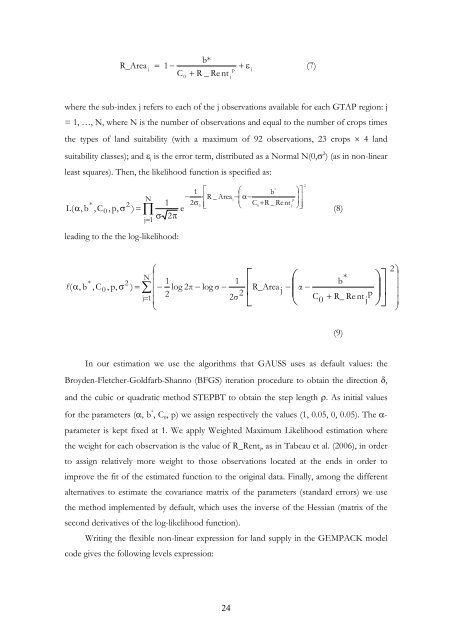
*<br />
R_Area j = 1 −<br />
+ ε j<br />
(7)<br />
C + R _ Re nt<br />
0<br />
where the sub-index j refers to each of the j observations available for each GTAP region: j<br />
= 1, …, N, where N is the number of observations and equal to the number of crops times<br />
the types of land suitability (with a maximum of 92 observations, 23 crops × 4 land<br />
suitability classes); and ε j is the error term, distributed as a Normal N(0,σ 2 ) (as in non-linear<br />
least squares). Then, the likelihood function is specified as:<br />
L(<br />
N<br />
1<br />
∏<br />
j=<br />
1 σ 2π<br />
j<br />
p<br />
* 2<br />
2 ⎢<br />
0<br />
j ⎥<br />
α , b , C , p,<br />
σ ) = e ⎣ ⎝<br />
⎠⎦<br />
(8)<br />
0<br />
leading to the the log-likelihood:<br />
*<br />
l(<br />
α,<br />
b<br />
, C<br />
0<br />
, p,<br />
σ<br />
2<br />
⎛<br />
24<br />
p<br />
j<br />
*<br />
1 ⎡ ⎛ b ⎞⎤<br />
− ⋅⎢R<br />
_ Area −⎜α−<br />
⎟⎥<br />
2σ<br />
⎜ C + R _ Rent<br />
⎟<br />
N ⎜<br />
⎡ ⎛<br />
⎞⎤<br />
⎜ 1<br />
1<br />
b<br />
*<br />
∑ − log 2π<br />
− log σ − R_Area − ⎢ ⎜ α − ⎟<br />
⎜ 2<br />
2 j<br />
⎥<br />
j 1<br />
C + R_ Re nt p<br />
⎜<br />
2σ<br />
⎣ ⎝ 0 j ⎠⎦<br />
= ⎟ ⎟⎟⎟<br />
) =<br />
⎝<br />
⎠<br />
In our estimation we use the algorithms that GAUSS uses as default values: the<br />
Broyden-Fletcher-Goldfarb-Shanno (BFGS) iteration procedure to obtain the direction δ,<br />
and the cubic or quadratic method STEPBT to obtain the step length ρ. As initial values<br />
for the parameters (α, b * , C 0, p) we assign respectively the values (1, 0.05, 0, 0.05). The α-<br />
parameter is kept fixed at 1. We apply Weighted Maximum Likelihood estimation where<br />
the weight for each observation is the value of R_Rentj, as in Tabeau et al. (2006), in order<br />
to assign relatively more weight to those observations located at the ends in order to<br />
improve the fit of the estimated function to the original data. Finally, among the different<br />
alternatives to estimate the covariance matrix of the parameters (standard errors) we use<br />
the method implemented by default, which uses the inverse of the Hessian (matrix of the<br />
second derivatives of the log-likelihood function).<br />
Writing the flexible non-linear expression for land supply in the GEMPACK model<br />
code gives the following levels expression:<br />
2<br />
(9)<br />
2⎞


