1 A Recursive Dynamic Computable General Equilibrium Model For ...

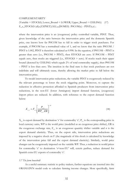
COMPLEMENTARITY
(Variable = STOCKS, Lower_Bound = LOWER, Upper_Bound = CEILING) (17)
E_c_STOCKS (all,c,EXPSET)(ALL,s,DOMES) P0COM(c) - PINT(c,s) ;
where the intervention price is an (exogenous) policy controlled variable, PINT. Thus,
given knowledge of the ratio between the intervention price and the domestic Spanish
price, one knows how far P0COM has to fall in order to trigger stock purchases. For
example, if P0COM has a normalised value of 1, and we know that the ratio P0COM /
PINT is 1.002, PINT is therefore calculated as 0.998. In the equation, if P0COM – PINT is
greater than zero (i.e., P0COM > PINT), then STOCKS are zero. If P0COM – PINT
equals zero, then stocks are triggered (i.e., STOCKS > zero). If stocks reach their upper
bound (denoted by CEILING which equals 2% of total commodity supply), then P0COM
– PINT is less than zero. The intuition in the final state is that stock purchases are not
indefinite and will ultimately cease, thereby allowing the market price to fall below the
intervention price.
To model intervention price reductions, the variable PINT is exogenously reduced by
the relevant percentage to lower the stock triggering point. Moreover, to capture the
reduction in effective protection afforded to Spainish producers from intervention price
reductions, in the non-EU (lower Armington) import demand function, (exogenous)
import prices are reduced. In addition, with reference to the export demand function
below:
X
= F
⎡ P ⎤ c,
s
⎢ ⎥
⎢⎣
WPc
, s.
ER⎥⎦
−σ
c,
s c,
s
(18)
Xc,s is export demand by destination ‘s’ for commodity ‘c’, Pc,s is the corresponding price in
local currency units, WP is the world price (modelled as an exogenous price shifter), ER is
the exogenous exchange rate, Fc,s is an exogenous quantity shifter variable and σ is the
export demand elasticity. Thus, on the export side, intervention price reductions are
imposed by a negative shock on F (the magnitude of this shock is calculated by knowledge
of the intervention price fall and the export demand elasticity). Similarly, world price
changes can be exogenously imposed on the variable WP. Thus, a reduction in world prices
for commodity ‘c’ to destination ‘s=non-EU’ will, ceteris paribus, reduce demand for
Spanish extra-EU exports of commodity ‘c’.
5.7 The farm household
As a useful summary statistic to policy makers, further equations are inserted into the
ORANI-DYN model code to calculate farming income changes. More specifically, farm
32