1 A Recursive Dynamic Computable General Equilibrium Model For ...

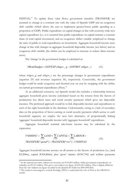
INDTAX). 31 To update these value flows, government transfers (TRANSFER) are
assumed to change at a constant rate with the value of Spanish GDP and an exogenous
shift variable (which allows the user to implement greater/lower public spending as a
proportion of GDP). Public expenditure on capital changes in line with economy-wide new
capital expenditure (i.e., it is assumed that public expenditure on capital remains a constant
share of total capital investment) and an exogenous shifter variable (employed to change
the ratio of public to total expenditures on investment). Aggregate household income taxes
change in line with changes in aggregate household disposable income (see below) and an
exogenous shift variable (the shifter can be employed to increase or reduce direct income
taxes).
The ‘change’ in the government budget is calculated as:
100. delbudget = GOVEXP.
w0gov
_ g − GOVREV.
w0gov
_ t (31)
where w0gov_g and w0gov_t are the percentage changes in government expenditures
(equation 29) and revenues (equation 30), respectively. Conceivably, the government
budget could be made exogenous and shocked year on year by swapping with the shifter
on current government expenditures (f5tot). 32
As an additional extension, our Spanish model also includes a relationship between
aggregate household gross income (calculated based on the returns from the factors of
production) less direct taxes and social security payments which gives net disposable
incomes. The prefereed approach would be to link disposable incomes and expenditures to
each of the eight households in the datrabase. Unfortunately, owing to a lack of secondary
data on the proportion of factor earning or social security payments which accrue to each
household segment, we employ the next best alternative of proportionally linking
‘aggregate’ household disposable income with ‘aggregate household’ expenditures.
Aggregate household nominal take-home income may be calculated by the
expression:
V 0HHINC
= ∑ LAND + ∑CAPITAL
+ ∑ LABOUR +
i=
IND
i=
IND
i=
IND
TRANSFER("
spend"
) −TRANSFER("
rev"
) −V
0HHTAX
(32)
Aggregate household income accrues on all returns to the factors of production (i.e., land
€9,208m), capital (€364,866m) plus ‘gross’ salaries (€430,734)) and welfare payments
31 In the national accounts, indirect tax revenues are €110,963 million, whilst government expenditures on
subsidies are €9,151 million. This gives a net indirect tax figure of €101,812 million. This is slightly different
from the ‘net’ indirect tax figure recorded in the Spanish IO Table for 2005 (€99,502).
32 The reader is encouraged to consult Horridge (2003) to understand the role of f5tot in the ORANI-G
model.
42